1. Introduction
Global energy consumption has been growing at 1.4% annually over the last 10 years [
1], and 94% of it is produced with combustion [
2]. Greenhouse gas emissions produce adverse effects on the environment and society and cannot be completely replaced. Buildings consume on average 40% of the electrical energy in European Union cities and 32% in world cities [
3], where the Heating, Ventilation, and Air Conditioning (HVAC) system requires 32.7% of the supplied electricity and up to 40.3% in public buildings [
4].
Advanced control systems improve energy management by adapting fast to unforeseen events or predicting system behavior. There are some examples of this, such as the application of neural networks with genetic algorithms in building management systems, reaching savings of 27% [
5]. Other studies improve the cost by 19.7%, adding an optimization module in the ambient controller [
6]. Some researchers have proven that it is possible to save 30% on cold days, embedding a machine-learning-based MPC controller [
7]. On the other hand, the faster the controller reaches the goals, the better the energy efficiency is obtained; for example, Adaptive LAMDA-PI (Learning Algorithm for Multivariable Data Analysis—Proportional Integral) controllers improve the Integral Absolute Error (IAE) of the response time by above 140% compared with conventional PI and Fuzzy-PI controllers [
8]. Optimization works are embedded in different tasks or problems of the HVAC systems in both design and operations. They are used to adjust Proportional, Integral, and Derivative (PID) controllers to improve the logic of Model-Predicting Controllers (MPCs) or to enhance the supervision tasks in the Building Management Systems (BMSs) or Multi-Agent Controllers (MACs) [
9]. There is a significant interest in embedding advanced, Artificial Intelligence (AI)-based control architectures in the BMS [
10] that provide acceptable results in uncertain contexts and complex systems, while allowing the adoption of multi-objective optimization policies. There are two visible advanced control strategies: (1) predicting the system behavior with machine-learning-based simulations to obtain the optimal sequence of instructions or (2) adapting the system parameters in case of context perturbances, so that it quickly returns to the zero-error state, such as with fuzzy logic control. Artificial Intelligence (AI), together with other technologies, such as Big Data, Internet of Things (IoT), or Cloud Computing, enhances the ubiquity, accessibility, mobility, knowledge extraction, and autonomy for the new software tasks. The traditional multi-objective problem in operations is to improve the energy efficiency and maintain comfort for the users, i.e., the ideal temperature, humidity, or Indoor Environmental Quality (IEQ) that mutually conflicts. Comfort, health, or maintenance add other objectives to the optimization problem, such as the CO
2 concentration, reducing the efficiency of the optimization with fewer objectives [
11].
Zadeh conceptually grouped under the umbrella of “soft computing” (SC) technologies that overperformed traditional deterministic approaches [
12], at the expense of losing accuracy and generalization. Thus, SC is tolerant to imprecision and uncertain approximation and today are widely used for complex problems where moderate precision and generalization capability are acceptable, given their high-resolution speed. SC covers three main fields: (1) Machine Learning (ML), (2) metaheuristics-based optimization, and (3) Fuzzy Logic (FL) for decision-making. Metaheuristics-based optimization [
11] offers good tradeoffs between consumed resources and accuracy for achieving global goals but brings challenges to face, such as algorithm convergence, stability, parameter tuning, a mathematical framework, benchmarking, generalization, and performance assessment [
13]. SC also offers fitness estimation for optimization with data-based models that require fewer computer resources [
14].
Digital transformation and the social trend towards standardization allow for sharing the functionality among different fields, requiring testing their approaches and convenience for specific applications. This conceptual ‘liquidity’ brings new challenges for optimization, such as the smart city, smart districts, and smart building, which leads to the scaling of the control and supervision capabilities to upper layers (e.g., ISA 95 and IEC 62264 L2), but constraining the lower layers. More conflicting objectives, such as the Coefficient of Performance (COP), allow for the monitoring of subtle equipment degradations, achieving considerable savings in the life cycle of the installations [
15]. The system management is susceptible to becoming autonomous with the self-optimization organic function.
Thus, society, while aiming to enhance people’s wealth and comfort, is forced to save energy and reduce costs. Multi-objective optimization strategies can be applied at several levels in building systems, especially HVAC, that can run at bare equipment control, at subsystems management, or at a superuser level integrating systems, buildings, blocks, or districts. In this scenario, there is a greenfield to explore, including among others autonomic building management architectures that automatically adapt their decisions to contextual changes and continuously improve with the experience. The proposed study demonstrates different multi-objective optimization techniques under this scenario that include conventional conflicting goals of comfort, observable with the ambient temperature, and energy-saving, quantifiable with the subsystems consumption, and add two new objectives: (1) the maximization of the absolute value of COP, allowing for optimal performance in saving energy and, at the same time, an enhancement of the lifecycle of the equipment, something rarely explored in operations before [
16]; (2) the minimization of the rate of change in ambient temperature, which allows the system to enter into a steady-state mode since startup at nearly critical damping. The possibility for the system to automatically select the most appropriate algorithm is also proposed for the next research outcome. Although it was expected that the addition of conflicting objectives could reduce the efficiency of the optimization, the results show evidence of a wide field to be explored.
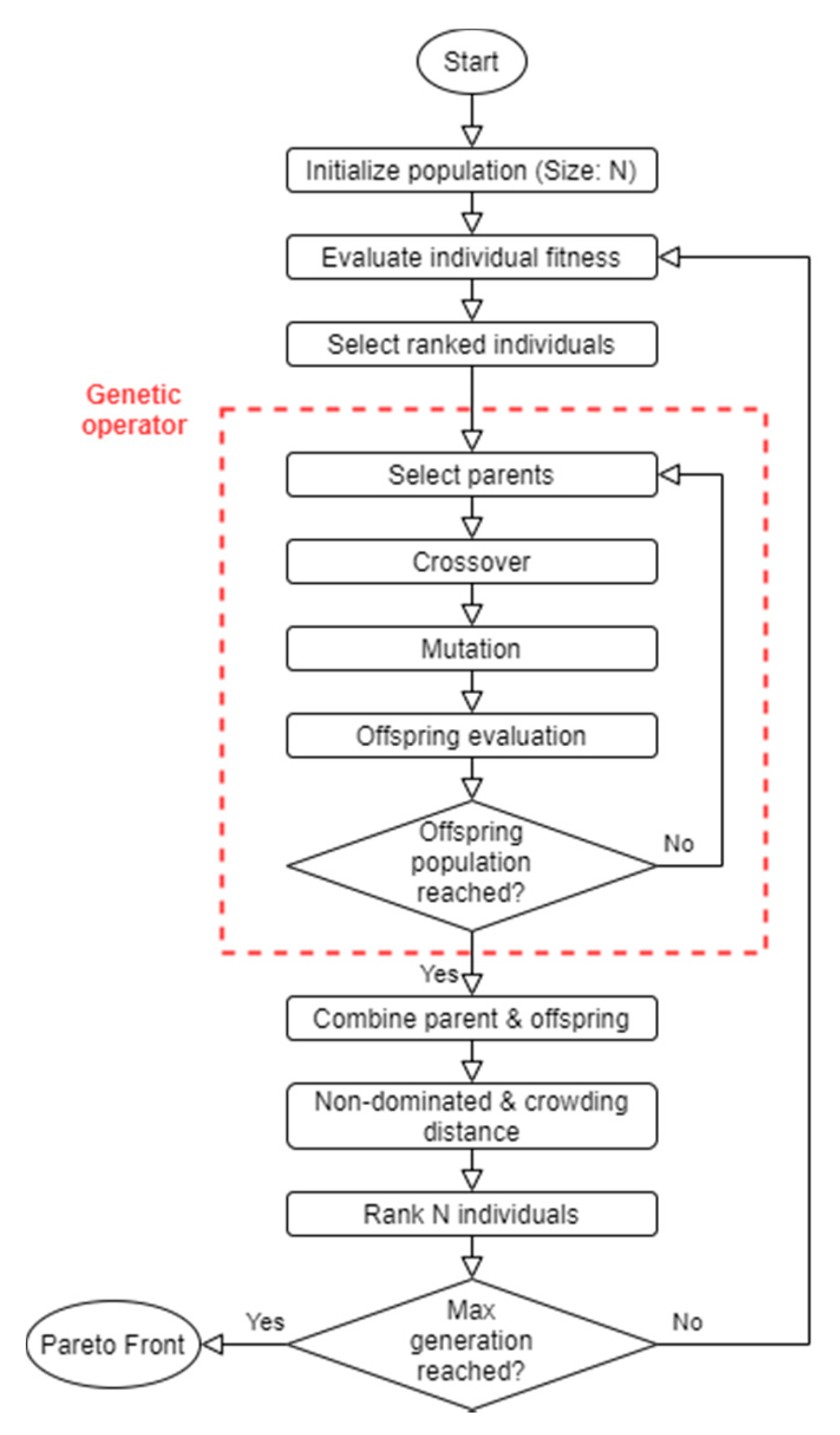
This comparative study shows the pros and cons of using different population-based multi-objective optimization algorithms for an HVAC control system. Current practices limit operation to ensure the comfort of building inhabitants dodging other objectives such as energy savings. The study will cover (1) Swarm Intelligence (SI) algorithms and (2) Genetic Algorithms (GAs) and will use real data from the HVAC system of Teatro Real de Madrid (Opera House). The individuals in the decision space are mapped in the objective space with cost functions empirically obtained with ML’s Random Forest Regressors (RFRs) to assess their dominance. The RFRs have been trained with a selection of data obtained from a historic database kindly provided by the Board of Teatro Real. The selected GAs are the Multi-Objective Genetic Algorithm (MOGA) and the Non-dominated Sorting Genetic Algorithm version 2 and 3 (NSGA-II and NSGA-III), and the selected SI-based algorithms are Optimized Multi-objective Particle Swarm Optimization (OMOPSO) and Speed-constrained Multi-objective Particle Swarm Optimization (SMPSO). In the experiment, the Strength Pareto Evolutionary Algorithm Version 2 (SPEA2) was discarded, as its execution time was excessive compared to the others. Random Search (RS) results are exhibited as a reference point.
The paper is organized as follows: In Related Work, the authors bring to light significant research related to this study. Materials and Methods explain how the experiment was built and the metrics for comparing the algorithms. The Results section visualizes and discusses the outcomes. Finally, the Conclusions section compares the obtained results with other studies, outlines the novelty, and proposes possible future research lines for this work.
2. Related Work
2.1. Towards a Clear Ontology
It is common for recent literature about SC and multi-objective optimization to take for granted the approach followed in this work, due to the absence of effective classification and, therefore, the formation of an adequate body of knowledge. Although it is beyond the scope of this study, it is prudent to indicate some examples of confusing terms and try to position them.
Non-preference multi-objective optimization, i.e., those finishing with a set of non-dominant solutions, is sometimes classified as a subset of ‘a posteriori’ decision-making, and sometimes they are synonyms. It is often associated with multimodal optimization, although only the latter also includes local search. It is also difficult to differentiate Evolutionary Computation from GAs. While sharing a similar process, a GA includes mating and crossover to improve the search. For some articles, they are synonyms and come grouped either as evolutionary or genetic. They are sometimes considered a subset of different approaches, such as bio-inspired algorithms.
Particle Swarm Optimization (PSO) can be classified itself [
17] or together with GAs [
18] under Multi-Objective Evolutionary Algorithms (MOEA). MOGA is sometimes considered a separated GA [
19] or the family of multi-objective GAs [
20]. MOEA and MOGA may include the whole metaheuristics-based search family or only those based on the population approach.
The new algorithms based on the observation of nature can be named bio-inspired, bio-search heuristics, or metaphor-based metaheuristics, among others, exchanging their different inspirations, be they biological, chemical, or physical. GAs or SI-based algorithms can be found included in the bio-inspired family, excluding the evolutionary algorithms [
19].
With regard to the optimization performance, it is possible to mislead concepts such as ‘convergence’ that could mean either to end the search at any point (lumps) or end it in true global optima. The diversity feature sometimes indicates the uniformity in the distribution of the solutions, how they spread, or both.
The classification by Ahma et al. [
9] and Oliva et al. [
21] with Zadec’s original SC definition [
12] supports the position of this study. At the top, algorithms are split up into stochastic techniques and intelligent agents (deterministic). Stochastic techniques then split into population-based and single individual algorithms (trajectory metaheuristics) that include Simulated Annealing (SA) and Tabu Search (TS). Population-based algorithms then split into SI and evolutionary algorithms. This study compares GAs (part of evolutionary algorithms) and SI-based particle swarms, PSO.
2.2. Research Interest
According to Wang, G. [
22], at an early stage, optimization methods diversified in different fields of study: (1) linear or nonlinear programming, (2) constraints, (3) single- or multi-objective optimization, and (4) dynamic programming. The first generation introduced the iteration and gradients. The second generation brought the metaheuristics-based search for global multi-objectives that reduced computing resources and allowed for parallel computation. Soft Computing (SC) AI approaches support surrogate-based or metamodel generation, replacing computer-aided simulation software with ML models. The next-generation links and hybridizes the above approaches.
Nabaei et al. [
23] provide a good reference for research interests in SI algorithms and GAs over time. GAs have been interesting since before 2000 with a peak from 2006 to 2010. PSO algorithms started to become comparable in 2006 and 2010, but there were much fewer articles published than there were regarding GAs, half of them spanning from 2011 to 2018. Another comprehensive study by Shaikh et al. [
11] illustrates the research interest for the optimization in building HVAC systems in which GA articles are 24% of the total and MOGA represent 3%. PSO is present in 5%, and MOPSO in 7%. Scheduling Optimization, Hooke and Jeeves, and Linear Quadratic shares range between 3% and 6%.
Optimization can be used for designing systems or in real-time operations [
24]. A GA is used for both design and operations, and so is NSGA-II, but only in a third of the articles reviewed. There are more articles about PSO in operations than in design, but a Differential Evolutionary (DE) algorithm is only used in designing, and the number of articles about the combination of these algorithms is similar to the number of articles related to NSGA-II.
2.3. Genetic and Swarm Intelligence Outcomes
Algorithms based on metaheuristics are good options for characterizing the behavior of complex, dynamic, and nonlinear systems [
25].
A GA puts together a set of individuals (chromosomes) ‘coded’ with genes (variables), marking them with fitness functions. It then uses a selection strategy to obtain a new population ready for the next iteration. Mutation and crossover operators regulate the speed and variety of chromosome changes in the GA. While the crossover ‘exploits’ the search, the mutation widens the explored space. One key point is the adjustment of the parameters to the specific problem. The mutation operator can generate solutions with polynomial or uniform probability distributions. The non-uniform probability prevents the population from decaying in the early stages of the evolution by generating distant solutions with a random probability. Simulated Binary Crossover (SBX) generates offspring from two parents attending to their probability distributions.
GAs discovers the optimal set in three different ways [
26]. (1) The first approach is known as Pareto-based dominance with a two-level ranking scheme, one to obtain the dominance and diversity assessment and the other, containing such metrics as the total nondominated vectors generation, the hypervolume, the generational distance or spacing, and the error rate [
27], to determine the convergence to local or global minima [
28]. NSGA-II and SPEA2 make use of these principles. (2) The second approach uses unary or binary indicators to check their performance, for example, with the coefficient of determination, the R2-like S-Metric Selection Evolutionary Multi-Objective Optimization Algorithm (SMS-EMOA) that maximizes the hypervolume (HV). (3) The third approach is based on decomposition that splits the overall problem into smaller problems for the search. There is not a common procedure for these algorithms. Splitting up complicated Pareto Fronts (PFs) to apply a local search and Tchebycheff’s scalarization is one of these methods, as well as the Multi-Objective Evolutionary Algorithm based on decomposition (MOEA/D) and NSGA-III.
The advantages of GAs are that they (1) have simple fitness arrangement schemes; (2) do not need derivatives or gradients; (3) are relatively robust; (4) are easy to parallelize. However, although they require less information about the problem, (1) designing an objective function, (2) getting a representation, and (3) adjusting the operators can be a difficult task. In addition, they are computationally expensive compared with others. NSGA and NSGA-II perform niching, decide deterministically the tournaments, and avoid chaotic perturbations of the population composition with updated fitness sharing. However, the niching function is too complex and scales poorly as the number of objectives increases [
24].
SI-based optimization is also population-based, where its individuals are bio-inspired on natural ecosystem metaphors, such as ants, bees, or particles [
29]. Swarm algorithms still generate some skepticism because of the mentioned metaphoric ornaments describing their operators [
30].
In the case of PSO, the particles move around in the decision space with simple mathematical equations that yield their position and velocity. Each particle’s best-known local position and velocity determine its movement towards the optimum. PSO (1) is easy to adjust; (2) can be implemented and provide fast speed results; (3) is capable of finding the global optimal solutions in most cases. However, (1) strict convergence cannot be assured; (2) they are relatively weak in terms of local search abilities; (3) in multi-modal problems, they are prone to obtain local optima [
23].
2.4. Research Activity
There are two schools of thought for improving the efficiency of population-based optimization. One focuses on balancing the explore and exploit strategy with many variations, such as the elitist strategy found in some GAs. The other seeks simplification, as decisions cannot be well understood, especially for large search spaces, discontinuities, noise, or algorithms with time-varying parameters, such as PSO. The revision of the research activity is guided by the following goals:
to find which metaheuristic among some GAs and SI algorithms performs better and discover possible ways for the system to automate the decision among them;
to study multi-objective optimization in the transient time at the startup of HVAC systems;
to include new optimization objectives for enhancing the lifecycle of the equipment and specifically to facilitate the transition to the steady state.
Sharif et al. [
31] included the assessment of the lifecycle cost (LCC) in addition to the energy consumption and environmental impact as a new optimization objective in the passive and active building design with a GA. They managed conflicting objectives such as renovating the envelope (passive structure) or the systems (active structure). Lee [
32] also combined a GA with Computational Fluid Dynamics (CFD) for the building geometry (passive design) and the HVAC system (active design), having the temperature, energy consumption, and the Index of Air Quality (IAQ) as objectives.
Gagnon et al. [
33] compared the computational resources spent in sequential and holistic approaches of a net-zero building design, using NSGA-II to optimize the carbon footprint, lifecycle cost, and thermal comfort. The experiment proved that the holistic approach achieved 59% of the optimal solutions in 100 h, and the sequential approach achieved 41% in 765 h.
The work of Haniff et al. [
34] is representative of introducing minor changes to an algorithm that improves the addressed problem. They modified the Global PSO so that it can outperform the optimization of the energy consumption and the temperature, considering the weather forecast, an estimation of the characteristics of the building, and the Predicted Mean Vote (PMV) for Air Conditioning scheduling.
Cai et al. [
35] proposed hybridizing a multi-objective evolutionary algorithm with a quantum-behaved PSO after dividing the problem into subproblems with Tchebycheff’s decomposition: Decomposition-based Multi-Objective Binary Quantum-behaved Particle Swarm Optimization (MOMBQPSO/D). The algorithm minimizes the temperature mean and deviation in area-to-point heat conduction.
Zhai et al. [
36] enhanced MOGA for the secondary cooling process in continuous casting by dynamically tuning the mutation and crossover operators with the probability method. They compared it with MOPSO and MOGA and showed a 10% water reduction.
Oliva et al. [
21] reviewed different metaheuristics-based algorithms applied to the estimation of solar cell parameters. They outlined the advantages and disadvantages of the GA, Harmony Search (HS), Artificial Bee Colony (ABC), SA, Cat Swarm Optimization, Differential Evolutionary, PSO, Advanced Bee Swarm Optimization, Whale Optimization Algorithm (WOA), Gravitational Search Algorithm, Flower Pollination Algorithm, Shuffled Complex Evolution, and Wind-Driven Optimization. They concluded that WOA performs better than the others regarding the accuracy and convergence speed and avoided local minima trapping.
Aguilar et al. [
37] proposed a new flexible architecture for Building Management Systems (BMSs), with an Autonomic Cycle of Data Analysis Tasks (ACODAT) that makes use of banks of optimization algorithms for HVAC system control and hinted at its use for supervisory and self-optimization tasks. In fact, in a later study, they developed a Fault Detect and Diagnosis (FDD) system optimized with MOPSO, also capable of long-term equipment degradation, using the COP [
15].
Awan et al. [
17] analyzed the design of a solar tower plant using fuzzy goals with PSO, showing significant improvements in most of the design parameters (solar multiple, tower height, and others).
Afzal et al. [
38] compared the results of applying Fuzzy Logic (FL) in both a GA and PSO to optimize the Nusselt number, friction coefficient, and maximum temperature of a battery thermal management, observing that GAs provide better results, though they are less widespread than PSO.
Suthar et al. [
39] compared NSGA-II, NSGA-III, and MOPSO, applying the Technique for the Order of Preference by the Similarity to Ideal Solution (TOPSIS) for tuning the parameters of a 2 Degree-of-Freedom (DoF) controller: the setpoint track, flow variation, and input fluid. The performance was measured with IAE, ISE, ITAE errors, and the execution time, and the step function reaction was analyzed.
Waseem Ahmad et al. [
9] assessed several optimization methods and indicated that GAs perform global searches well but show poor convergence. Swarm-based algorithms are good for local searches but are slower than genetic algorithms for global searches. However, Ant Colony Optimization (ACO) is faster at searching compared to others and at converging compared to simple genetic algorithms. In an HVAC system’s control, the most studied multi-objective optimization techniques are GAs, in 29% of the related literature, and MOPSO, in 10%. MOGA also stands out among them.
Behrooz et al. [
40] confirmed that GAs provide optimization for comfort and energy savings because of their good behavior with nonlinear systems but are challenged with variable context information and perturbances [
41]. They are sometimes combined with fuzzy control [
8].
Previous and current research does not fully cover the topics addressed in this article, which constitutes a novelty. Most of the studies demonstrate GA and SI optimization in HVAC systems in both design and operations, but few compare them. Some research deals with dynamic adaptation, such as dynamic PID tunning, but none of them include optimization of the COP to enlarge the lifecycle and the rate of change in ambient temperature at the end of the transient state to moderate the damping to a steady state.
Table 1 shows all cited works related to this section.
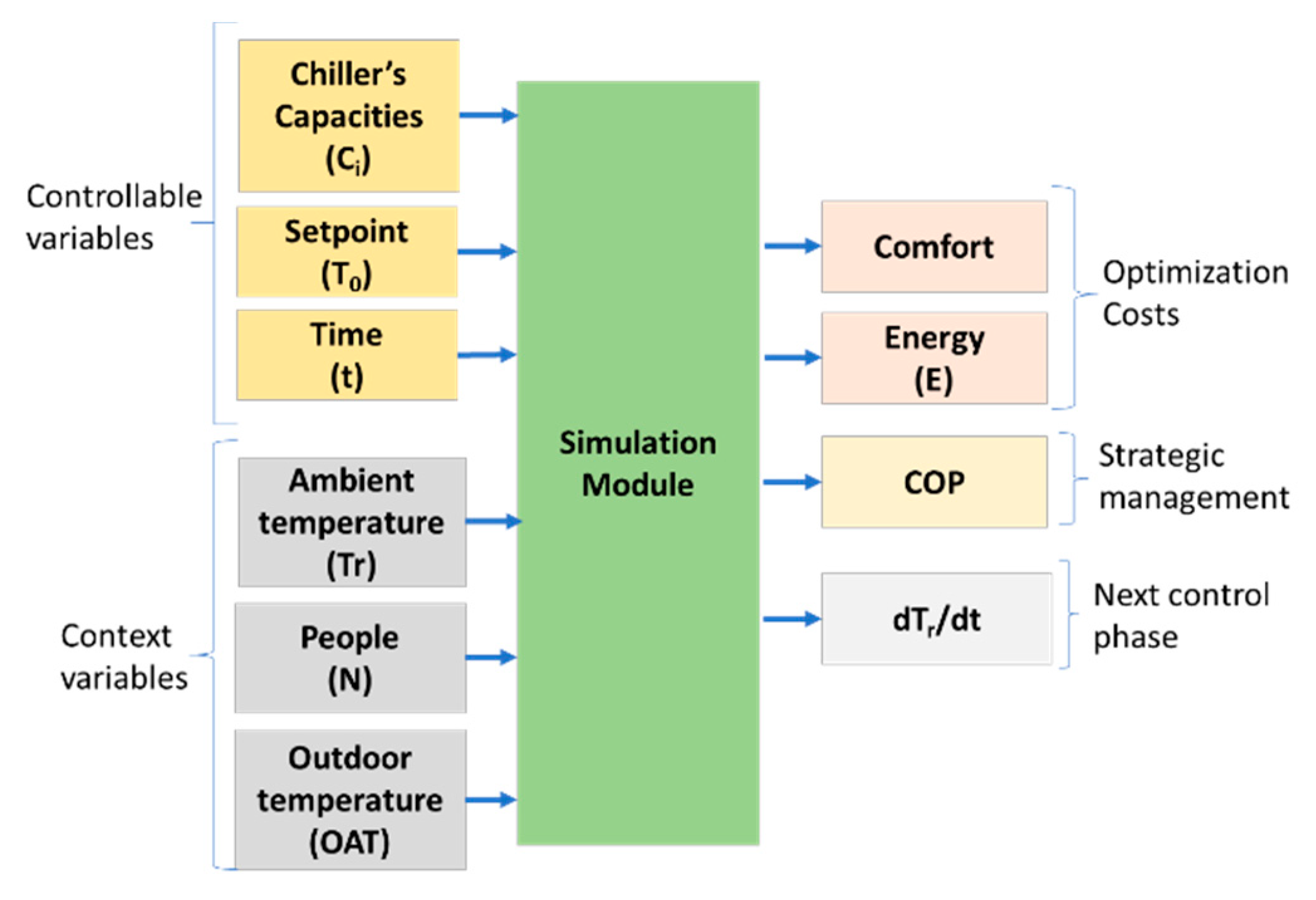
4. Problem Formulation
The HVAC system of Teatro Real is set to follow the mechanical and comfort setpoints required for a near event. The time spent to climatize and several HVAC parameters are those that the chiller’s manufacturer initially recommended just after installation. The BMS sends commands to the HVAC system to start/stop the chillers in a certain sequence to ensure that, at the time of the event, the comfort parameters will be appropriate.
The proposed control loop for the multi-HVAC system performance optimization is depicted in
Figure 5.
The Control Module, with the same functions as today, initiates the process by requesting the Optimization Module for instructions to improve its operation. The Optimization Module, which performs a metaheuristic search in the space of possible solutions, returns the best candidate obtained with the algorithm used in each model run (either with GA or SI). The fitness functions of the candidates are evaluated by the Simulation Module that receives every individual of the population and performs the simulation of the HVAC behavior (non-linear system) [
53], as defined by the candidate control parameters. The simulation is carried out with an ML algorithm, specifically a Random Forest Regressor (RFR), previously trained with historical data from the database of Teatro Real, by minimizing the Mean Squared Error (MSE) and maximizing the coefficient of determination (R
2). The RFR also requests contextual information to compute the simulation, which is provided by external sources. Finally, the Control Module translates the optimal recommendations into instructions for the actuators.
Each experiment carried out in this study executes one control cycle (petition) and addresses the optimization, without delving into the control stage. Inspired by the ACODAT management architecture for HVAC systems [
37], an autonomous cycle updates the model offline, maintaining its accuracy in real operational conditions, as shown by the green arrow in
Figure 5.
The primary objectives are to maximize comfort and minimize the consumed energy.
where T
0 is the setpoint temperature, and T
r is the indoor room temperature, both in °C. The maximum comfort for the optimization is therefore 0. The consumed electrical energy, E, is the sum of the consumed energy in kW.h in each chiller group, the multi-HVAC concept [
37]. N is the number of chiller groups. The energy of one chiller group, E
i, is
where E
chiller,i is the energy consumed in the chiller machine, E
CT,i is that in the cooling tower, E
cwp,i is that in the cooling water pump, and E
wpp,I is that in the chilled water primary pump.
This study includes two new objectives in the optimization as a novelty. The first one is the Coefficient of Performance, COP. The higher the COP is, the better the performance of the equipment, resulting in better energy efficiency and lower maintenance costs:
The COP is the engineering ratio of the supplied thermal power, W, to the consumed electric power, P. The optimization of the COP brings two important advantages for the HVAC system. HVAC equipment is designed to work at maximum performance, and in this regime, the system obtains its best energy efficiency. With the appropriate autonomous cycle of data tasks [
8], the supervisory system detects the degradation of the system, providing predictive maintenance [
15].
The second novel objective is the rate of change in the ambient temperature,
, that is the rate at which the temperature varies when it reaches the setpoint. This objective leads the system to rapidly reach the steady state with convenient damp that minimizes the overshooting:
This parameter is important at sudden startups when there is a transient time before the steady state [
16]. The lower the slope of the derivative is, the less impact on overshooting and steady noise there is on the next control phase.
The optimization requires Comfort, E, and
to be minimized and COP to be maximized. The decision space is formed with the chillers’ capacities, C
i [%], the setpoint, T
0 [°C], and the schedule or the date and time at which the system is expected to reach the setpoint, t
start. The indoor ambient temperature when the system starts, T
r(t = 0) [°C], the number of occupants, N, and the outdoor ambient temperature, OAT [°C], are the contextual information that determines the system. This study uses the capacity of the chillers as actuators on the subsystems, and this is justified with this simplified model:
where P
i is the electrical power actually supplied from the ith chiller, and P
max is the maximum power of the chiller. The chiller’s thermal power is generated according to the machine performance that is added to the other chillers, W
HVAC.
Thermal power conditions indoors compensate for the outdoor weather conditions and the corporal temperature of the occupants:
The thermal energy, Q, is then obtained from the power, and
is obtained from
, the indoor temperature variance.
Figure 6 shows the model with the inputs required, grouped in controllable and control variables, and the outputs, differentiating the normal optimization objectives of the thermal inertia for the next control plan [
37].
An individual in the population consists of a sequence of four operational modes of the chillers based on their capacities, C
i [%], at certain times, t
i, before the event starts at t
end [
37]. Each operational mode is a 5-tuple consisting of the proposed capacities for the four chillers ranging from 0% to 100% and the time that they start. Thus, a single individual contains four of these 5-tuples. The RFR performs a simulation for each 5-tuple, chaining them according to their start-up time. The last 5-tuple indicates the operational values applied to the chillers until the system reaches the steady state, t
end.
The multi-objective optimization problem would be formally defined as follows:
- 1.
Find the vector
in the decision space:
t
i, where i = 1, 2, 3, and 4, represents the starting dates and times to configure the capacities of every subsystem, while
, where j = 1, 2, 3, and 4, represents the capacities of the chiller j during the period that starts at i and ends at i + 1. The last period is between t
4 and t
end.
- 2.
will satisfy these inequality constraints at the following point:
- 3.
will optimize the vector function
in the objective space:
Comfort and COP must be maximized, while consumed energy, E, and the rate of change of ambient temperature, must be minimized.
5. Results
5.1. Dataset
The BMS is connected to 1824 digital and analog sensors, prompting the ambient and return temperatures, frozen water flow rates, valve states, chiller’s performance, secondary circuit values, air flow rate, fan speeds, pumps rotational speeds, controller status, etc., and allows the operator to send instructions to the actuators from the centralized platform. However, the historical data only keeps 169 variables: outdoor temperature, room temperatures, electrical supplied power, thermal energy generated by each of the four HVAC subsystems, and their COPs grouped in several tables with different sampling rates (10 min, 15 min, 1 h, daily). Usable records are from January 2016 to June 2018. The data have been cleaned to improve the accuracy by removing nonessential fields, records with outliers, nulls, and/or zeros, getting 9898 (80%) registers for training and 2475 (20%) for validation.
The Department of Engineering prepares the work order, based on the HVAC operational mode (HOM) for the field operators based on the events schedule and the weather forecasts, and consisting of pre-programmed routines. This is, however, inefficient because the complexity of the system operation reduces all possible variations to a small set of HOMs, based on the primitive recommendations of the installers. The occupancy of the building can reach up to 1700 during performances, while the number of people on labor days is around 600.
5.2. Data Model
The multi-objective estimation is computed with the RFR with good accuracy and speed balance. The model simulates the outputs in intervals of 15 min, which is a tradeoff between the system inertia and the discretization of the system dynamics. The model receives the time required for starting up the HVAC system, t
0, the time of the venue or the moment in which the room temperature, t
end, must reach the setpoint, T
0, the room temperature at the beginning, T
r (t = t
0), the number of people, N, and the outdoor temperature forecast, which is a vector of temperatures from t
0 to t
end every 15 min.
Table 2 represents an example where the temperature at 17 °C must reach the setpoint, 23.5 °C, in an hour.
The model also requires the outdoor temperature from the weather forecast. The optimization algorithm then releases the proposed individual for fitness.
In addition, the simulation receives the set of HOMs searched by the algorithms that will work in each interval. The algorithm is a sequence of HOMs proposed for the slots in the interval from t
0 to t
end, consisting of the power capacities of each chiller. Following the example,
Table 3 shows one of these candidate solutions.
A negative capacity indicates that the chiller is cooling, while a positive one indicates that it is heating. Real implementations will impose restrictions that are not considered here, such as smoothing the capacity transitions from one slot to another or preparing the chiller for cooling or heating modes.
Table 4 depicts the result of the optimization for this example.
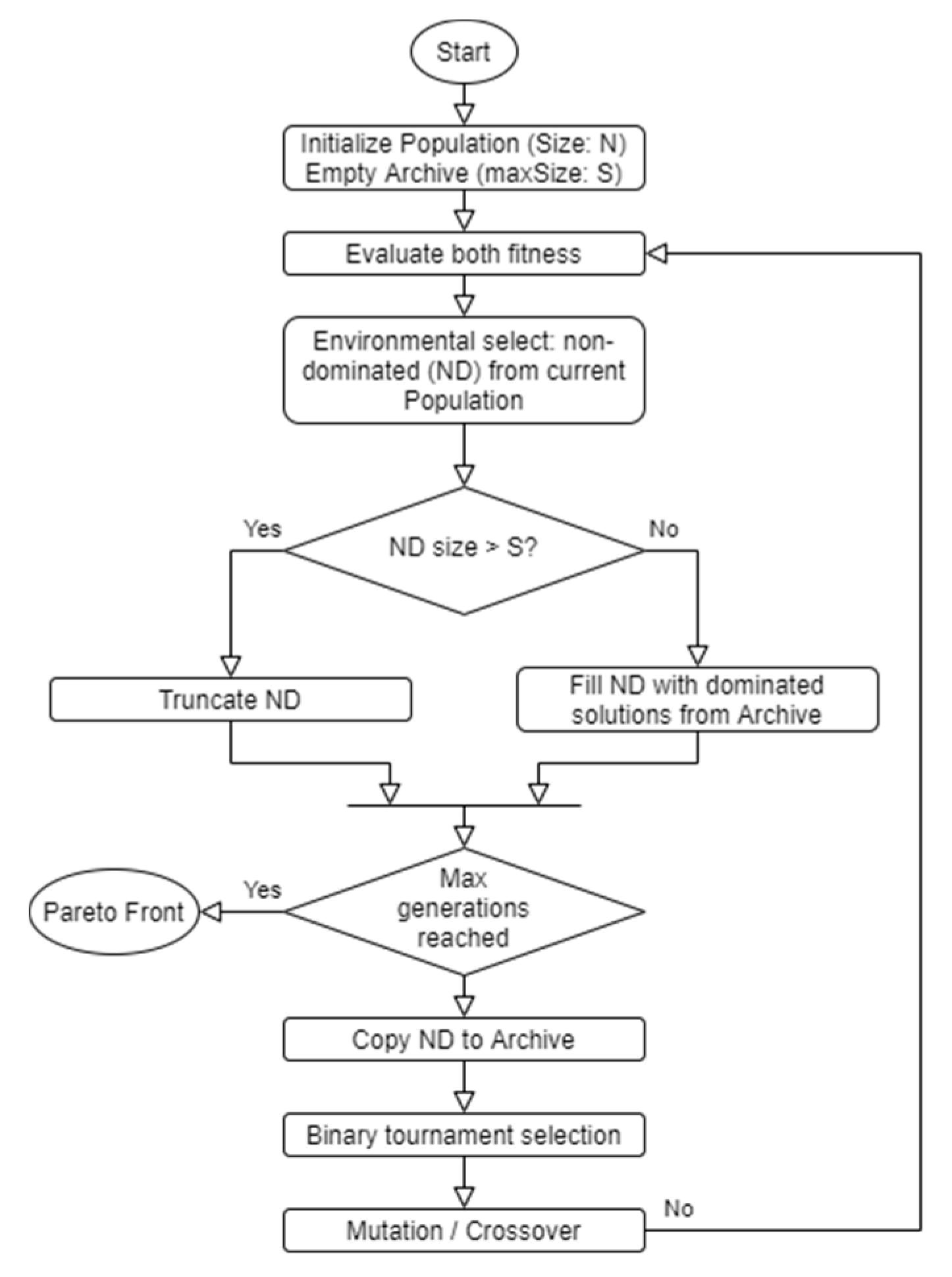
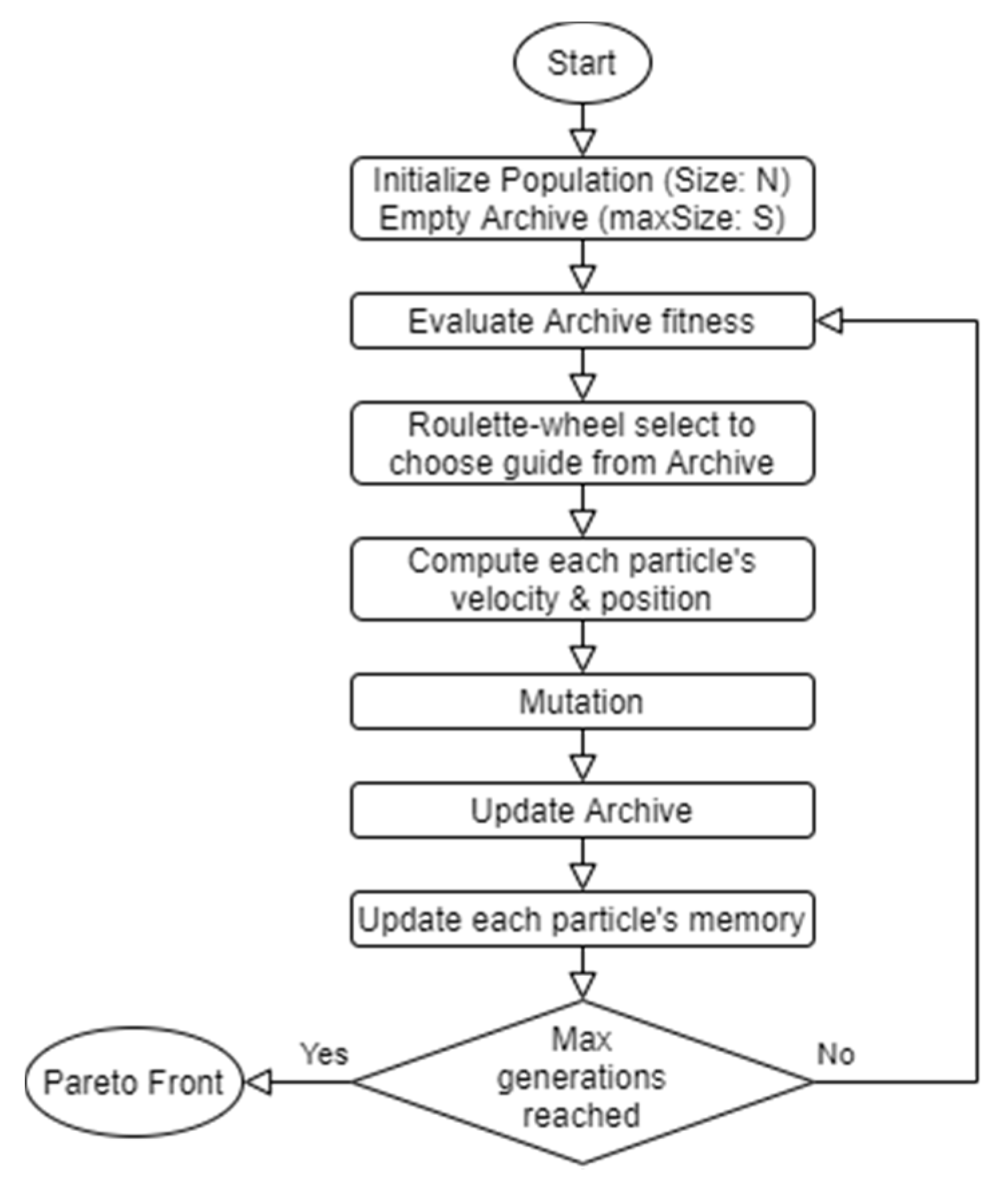
5.3. Algorithm Analysis
The analysis compares the performance and execution time (ET) of the algorithms. They start with the same expected number of solutions, i.e., the population size for the GA and the swarm size for the SI algorithm. The experiment involved population/swarm sizes ranging from 100 to 350 in steps of 50. The mutation probabilities were the same, and the SBX crossover probabilities and distribution index were the same for the GAs. The mutation scheme followed a polynomial probability distribution, except for OMOPSO, which combined uniform and nonuniform distributions with the same perturbation index, 0.5.
The algorithms stopped after 5000 iterations, and GAs stopped earlier if they were triggered with the dominance threshold. In order to obtain stable results, the algorithms were proved 10 times to determine the average of the obtained values.
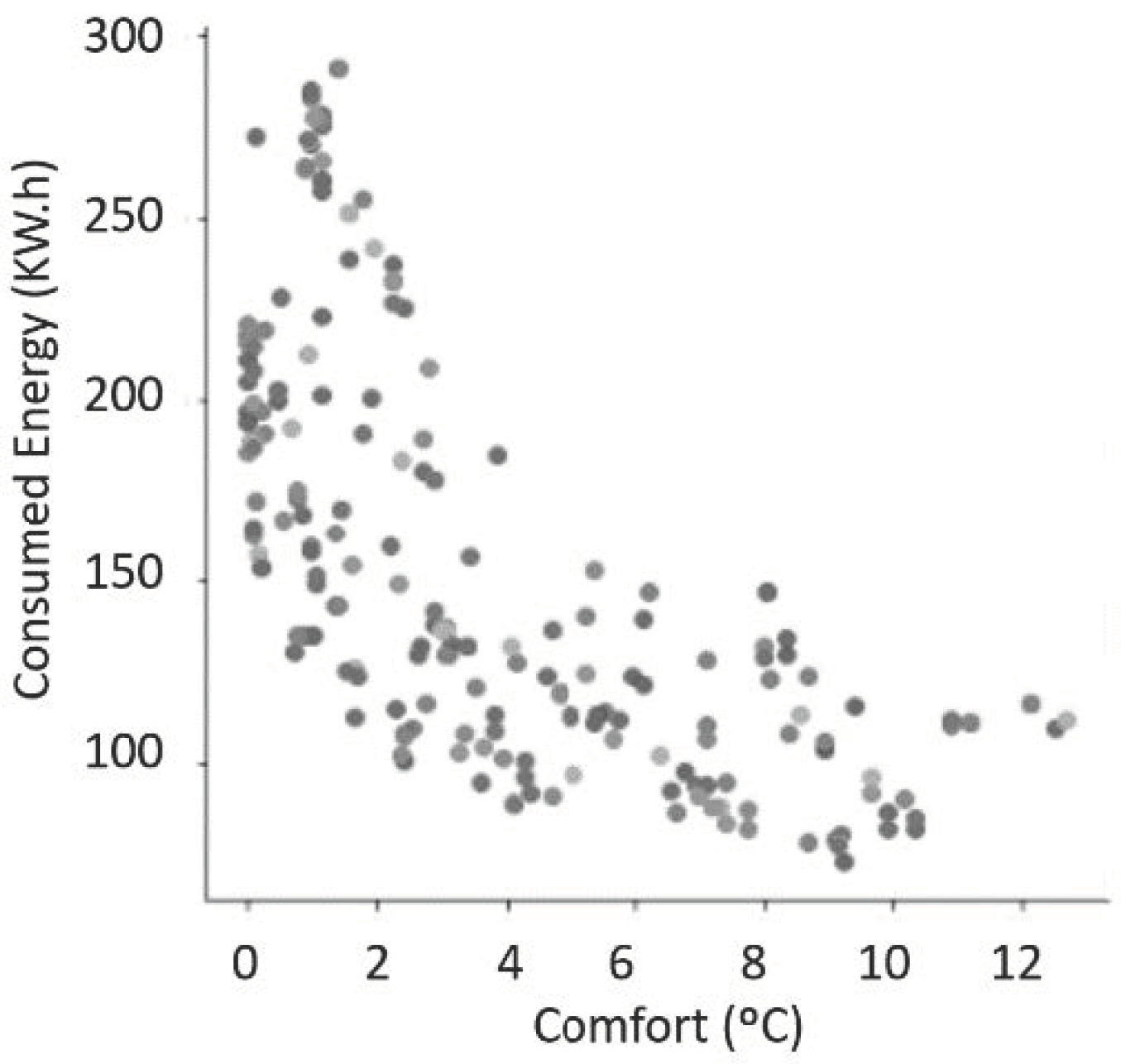
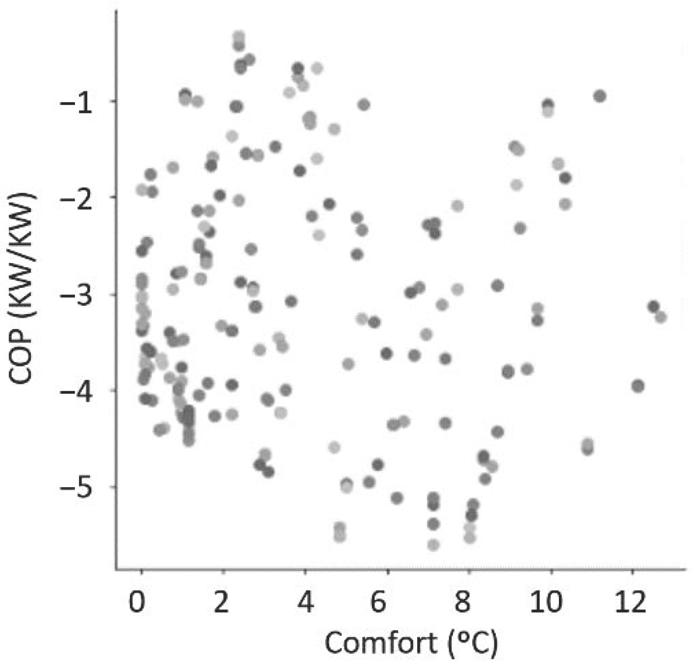
Figure 7,
Figure 8 and
Figure 9 represent the objective space for the variables Comfort, Consumed Energy, and COP in 2D diagrams.
Metrics used in the comparison were computed with the JMetal framework, and the ETs were recorded. The SPEA2 algorithm was dropped from the analysis, as it takes 22-fold more runtime than MOGA [
45].
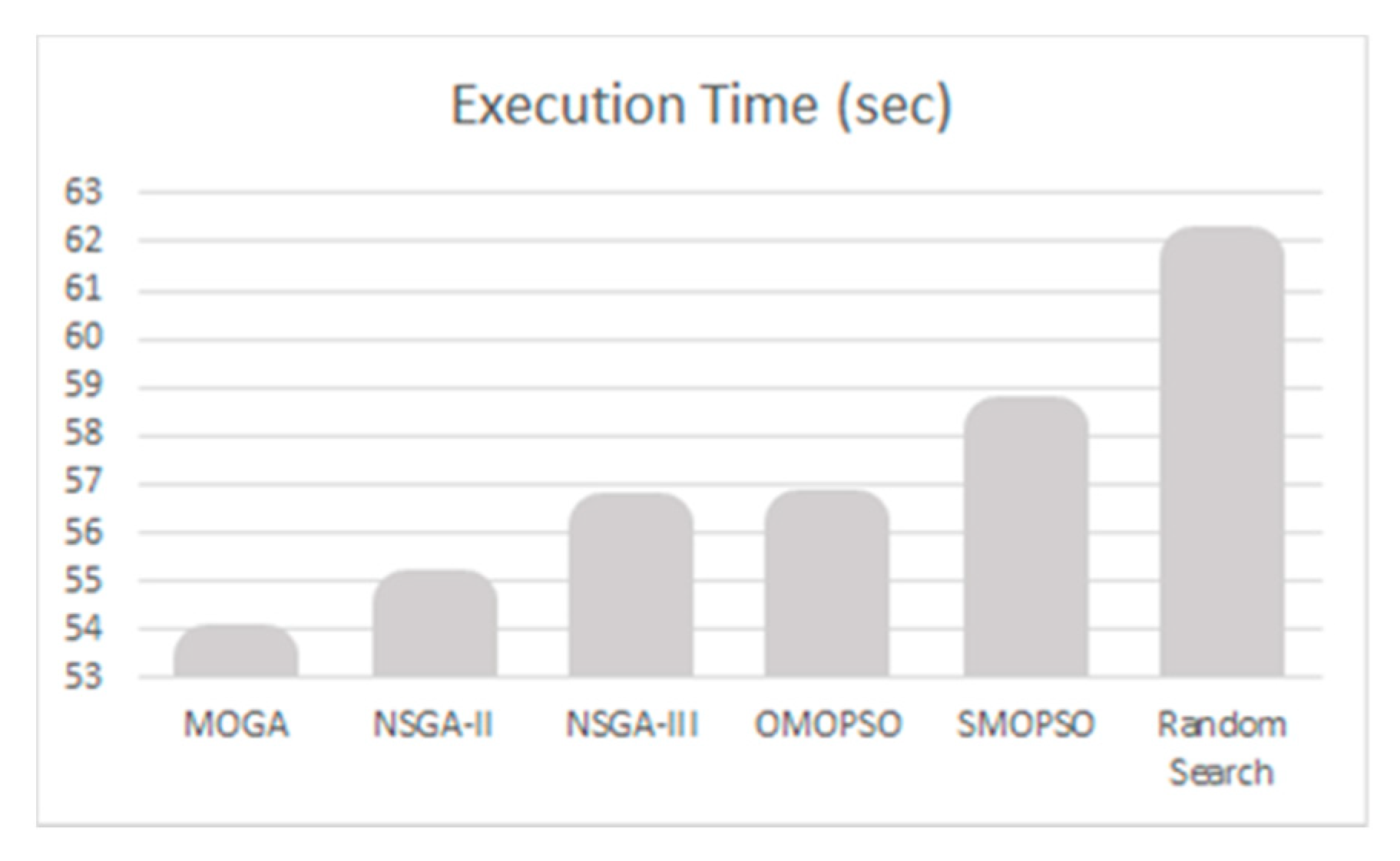
Figure 10 shows the obtained ET values.
The GAs ran faster than the SI-based algorithms. MOGA improved the Random Search by 13%, and OMOPSO improved it by 9%. It was observed that NSGA-III takes more time than NSGA-II to execute. This is because of the extra computation required for the adaptive operator and the generation of hyperplanes. On the other hand, the speed constraint mechanism seemed to increase the ET of the SMPSO, compared with OMOPSO. All outperformed RS.
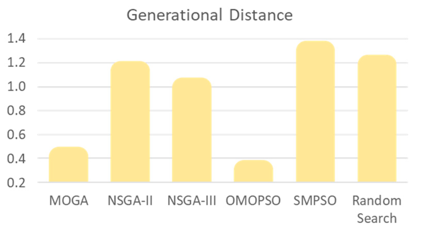
GD showed how close the fitness of the set of solutions was from the ideal PF, and this is depicted in
Figure 11.
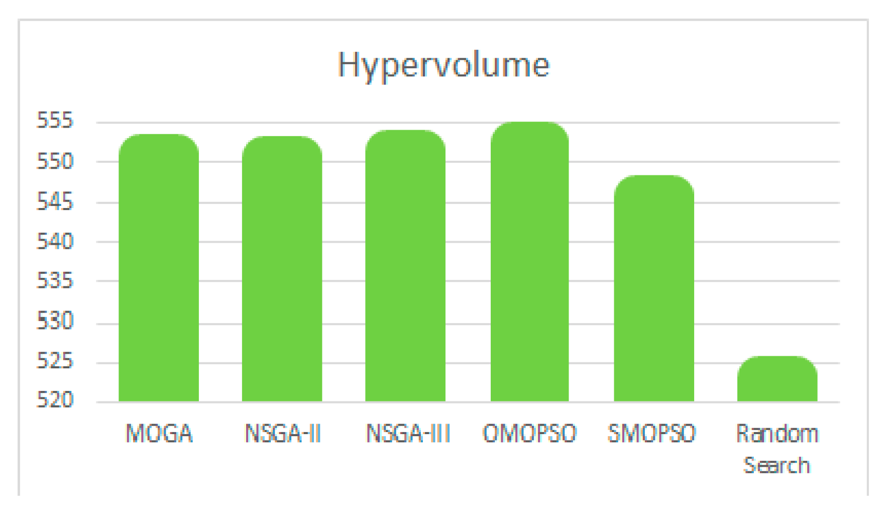
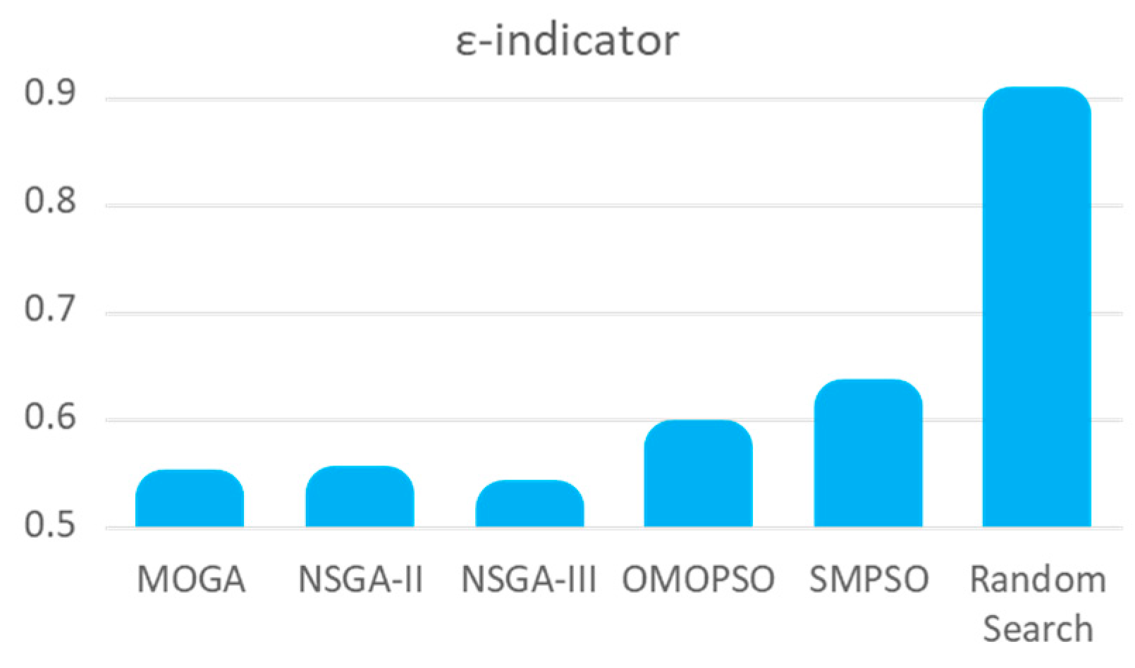
An approximate PF was constructed running the NSGA-II 20,000 times, simulating a limit behavior. The accuracy of OMOPSO and MOGA with 75% and 65% improvements compared to Random Search was observed. It was unavoidable that the quasi-ideal PF construction was insufficient for the rest of the algorithms. HV and EI are shown in
Figure 12 and
Figure 13.
In both metrics, it is possible to identify the significant improvements of all the algorithms compared with Random Search. The ε-Indicator show NSGA-III and MOGA as the best algorithms, outperforming Random Search by 42% and 40%, while the SI algorithms were worse (31–35%). The HV does not show significant differences among algorithms but shows an improvement of 5% on average.
5.4. Visualization
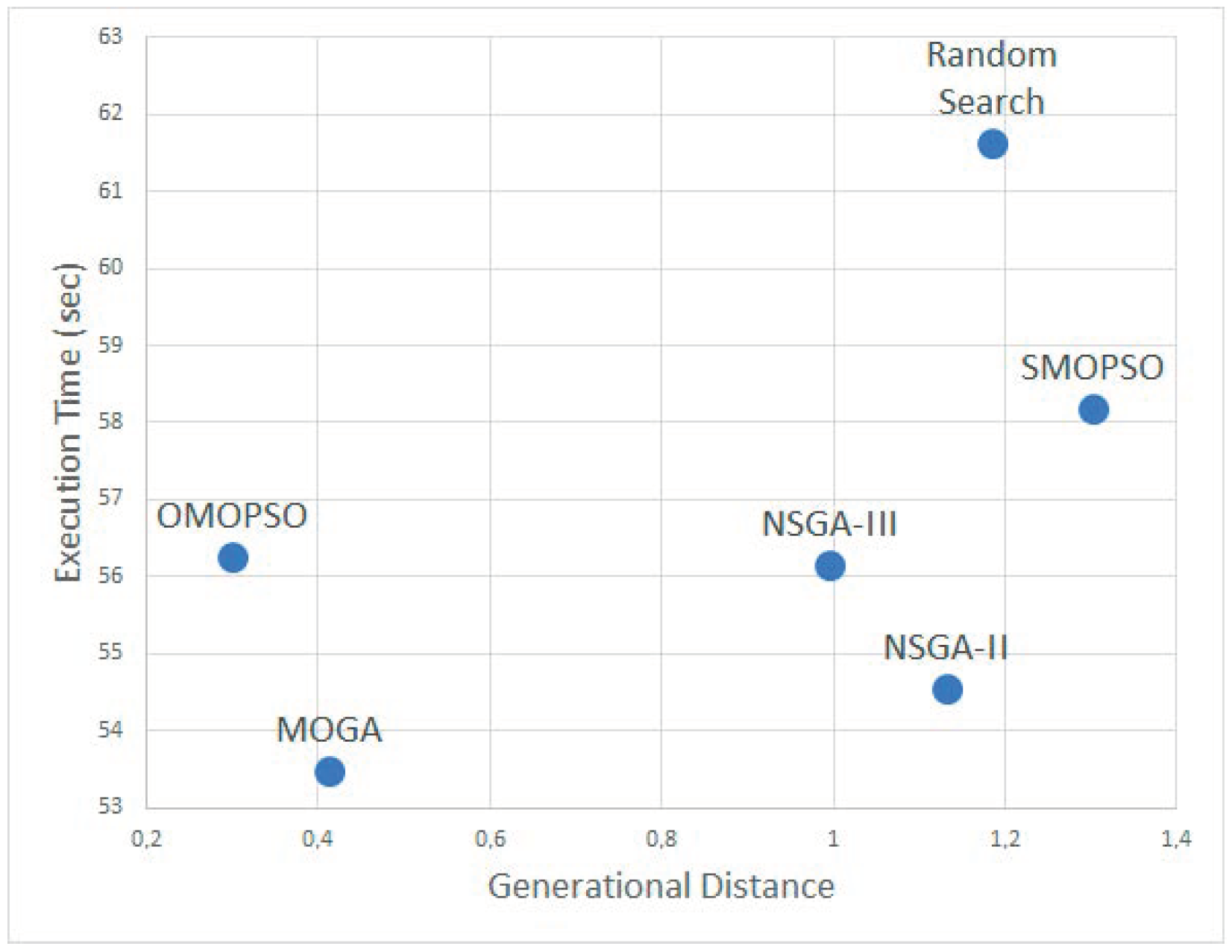
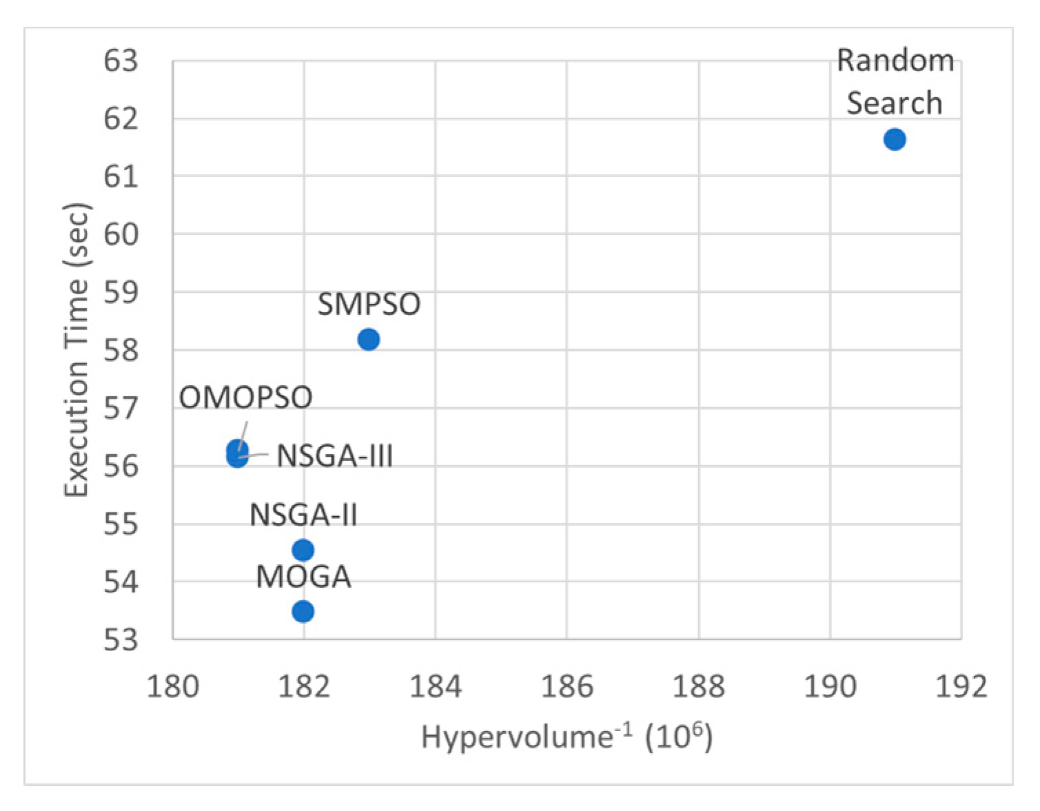
Regarding the question of whether an algorithm outperforms another with a combination of any quality measures, such as those seen above, Zitzler came to the conclusion that there was no such combination, but it could be seen as the equivalence to the concept of dominating [
54]. Thus,
Figure 14,
Figure 15 and
Figure 16 show 2D maps formed with the metrics of this study, those closer to the bottom left corner being the most appropriate. The best algorithms are found in the lower-left corner in all cases. The charts also show the distance among them, presenting an intuitive method with which to make decisions as to which performs better.
Figure 14 shows the behavior of the algorithms when setting the priority in ET and GD.
This case yields the selection of either MOGA or OMOPSO algorithms as the best for optimization accuracy. Both metrics penalize SMPSO, which obtains a GD even worse than RS.
Figure 15 prioritizes the HV (the inverse in this case for obtaining a homogeneous visualization) with the ET.
In this case, SMPSO still performs worse than the others in terms of accuracy, but much better than RS, likely due to diversity. All the rest behave similarly, the GA family standing out.
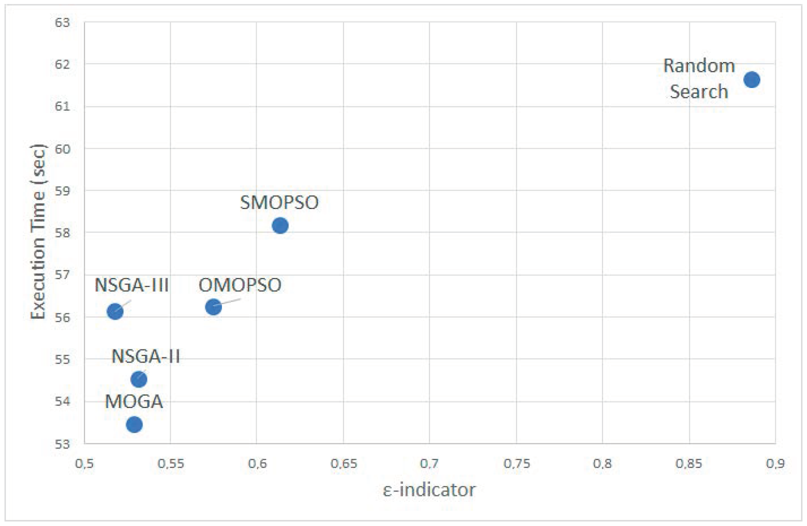
Figure 16 prioritizes the ε-Indicator and ET.
ε-Indicator also measures the cardinality and maintains SMPSO at the back, followed by OMOPSO, while GAs shows better behavior.
5.5. Energy Efficiency Improvements
To complete the experiment, four differentiated events available in the historical data of the building were randomly selected to compare the performance of the HVAC equipment in terms of energy efficiency, with the results that would have been obtained by applying the proposed optimization. This indicates what can be expected from this approach. The events are defined in
Table 5.
To illustrate the example, a second decision-making process with a weighted sum was set to select one of the solutions with values in the PF. Weights slightly favored Consumed Energy savings over the others.
Table 6 shows the results.
The right column shows the theoretical energy savings in each case with the optimized HOMs compared with what was actually recorded in the dataset. This column also stresses the achievements in comfort with expected deviations of less than 0.5 °C and HVAC subsystems working with COPs above 3.00, which is considered a good value. These impressive results of 60–80% in energy savings, preserving the comfort and the system performance, must be adjusted with further research considering real restrictions, but they hint toward a promising line of research.
5.6. Comparison with Other Works
Several authors have proposed comparisons between NSGA-II and MOPSO, which may contribute to the comprehension of the results. Keshavarz et al. [
55] compared NSGA-II and MOPSO for the stochastic optimization of an inventory control system, showing that NSGA-II has better performance in spacing and in the number of Pareto optimal solutions, while MOPSO better spreads the fitness of the solution set and consumes fewer computational resources. Niyomubyeyi et al. [
56] studied optimization in evacuation planning, obtaining better convergence and spread with MOPSO, but the algorithm execution took five times longer than NSGA-II. Saldanha et al. [
18] obtained similar results in convergence and spread for MOPSO and NSGA-II, although MOPSO yielded better results in spacing. Elgammal et al. [
57] studied the integration of hybrid wind photovoltaic and fuel cells, obtaining similar system operating costs with both, but in this case, the MOPSO execution time was shorter than NSGA-II.
6. Conclusions
This study shows the performance of several genetic and SI-based algorithms when optimizing the control of a building HVAC system. The study works with the real historical data of a complex and singular building by adapting the control logic to the available sensed measures and individual chiller actuators. The results yield that simple MOGA and NSGA-II/III run faster than MOPSOs, confirming the pure Random Search algorithm as the slowest. The best convergence is obtained with OMOPSO according to GD and HV.
The achievement on energy consumption is impressive, as shown with several events randomly selected from the data, reaching savings from 60% to 80%. These results will be proved for generalization purposes with further research that will include the new model’s restrictions.
This study is the first to take two new objectives into the optimization problem: the HVAC subsystem’s performance, COP, and the rate of change in ambient temperature at the end of the system startup stage. The first objective brings the possibility of advanced supervisory policies that improve the maintenance of the equipment and extend its lifecycle. The minimization of the second allows for a smooth transition to the permanent stage of the HVAC operation, reducing the overshoots or the underdamping effect of the room temperature values. In the following works, the dominance variation produced when adding new conflicting objectives and how this affects control system decision-making will be analyzed.
The proposed simple visualization of the algorithms not only allows for an intuitive understanding of which algorithm performs better but also opens the possibility of the automatic real-time instantiation of the most convenient algorithm from a bank of optimizers according to given contextual information. This is important because there are no rigid rules, but rather, existing or new strategies, such as running out of time, operations when the building is closed, etc.
The article also claims for consensus in optimization with a body of knowledge that integrates the contribution of the different disciplines that theorize or are applicable to the case.
This study requires generalization to demonstrate its scope with other different buildings, HVAC systems, and overall different variables extracted from the control logic. It is also of interest to work on parameter tuning to characterize the inherent “no free lunch” theorem.
The use of real data has made the study more reliable. The singularity of the building and the heterogeneous equipment that forms the HVAC system represents a demanding test for this research.
This research will contribute to the development of the smart city with autonomic management systems capable of learning from experience and improving with the context using AI to overcome the complexity of the managed systems and changing the user’s requirements.


 ,
, 


