Abstract
Worst-case scenario optimization deals with the minimization of the maximum output in all scenarios of a problem, and it is usually formulated as a min-max problem. Employing nested evolutionary algorithms to solve the problem requires numerous function evaluations. This work proposes a differential evolution with an estimation of distribution algorithm. The algorithm has a nested form, where a differential evolution is applied for both the design and scenario space optimization. To reduce the computational cost, we estimate the distribution of the best worst solution for the best solutions found so far. The probabilistic model is used to sample part of the initial population of the scenario space differential evolution, using a priori knowledge of the previous generations. The method is compared with a state-of-the-art algorithm on both benchmark problems and an engineering application, and the related results are reported.
1. Introduction
Many real-world optimization problems, including engineering design optimization, typically involve uncertainty that needs to be considered for a robust solution to be found. The worst-case scenario optimization refers to obtaining the solution that will perform best under the worst possible conditions. This approach gives the most conservative solution but also the most robust solution to the problem under uncertainty.
The formulation of the problem that arises is a special case of a bilevel optimization problem (BOP), where one optimization problem has another optimization problem in its constraints [1,2]. In the worst-case scenario case, the maximization of the function in the uncertain space is nested in the minimization in the design space, leading to a min-max optimization problem. Therefore, optimization can be achieved in a hierarchical way.
Min-max optimization has been solved by classical methods such as mathematical programming [3], branch-and-bound algorithms [4] and approximation methods [5]. These methods have limited application as they require simplifying assumptions about the fitness function, such as linearity and convexity.
In recent years, evolutionary algorithms (EAs) have been developed to solve min-max optimization problems. Using EAs mitigates the problem of making specific assumptions about the underlying problem, as they are population-based and they directly use the objectives. In this way, they can handle mathematically intractable problems that do not follow specific mathematical properties.
A very popular approach to solve min-max problems with the EAs is the co-evolutionary approach, where the populations of design and scenario space are co-evolving. In [6], a co-evolutionary genetic algorithm was developed, while in [7], particle swarm optimization was used as the evolution strategy. In such approaches, the optimization search over the design and scenario space is parallelized, reducing significantly the number of function evaluations. In general, they manage to successfully solve symmetrical problems but perform poorly in asymmetrical problems by looping over bad solutions, due to the red queen effect [8]. As the condition of symmetry does not hold in the majority of the problems [definition can be found in Section 2, they become unsuitable for most of the problems.
One approach to mitigate this problem is to apply a nested structure, solving the problem hierarchically as for e.g., in [9], where a nested particle swarm optimization is applied. This leads to a prohibitively increased computation cost, as the design and scenario space is infinite for continuous problems. Min-max optimization problems solved as bilevel problems with bilevel evolutionary algorithms were presented in [10], where three algorithms—the BLDE [11], a completely nested algorithm, the BLEAQ [1], an evolutionary algorithm that employs quadratic approximation in the mappings of the two levels, and the BLCMAES [12], a specialized bilevel CMA-ES—known to perform well in bilevel problems, were tested on a min-max test function and showed good performance in most of the cases but required a high number of function evaluations. A recently proposed differential evolution (DE) with a bottom-boosting scheme that does not use surrogates proved to reach superior accuracy, though the number of functional evaluations (FEs) needed is still relatively high [13].
Using a surrogate model can lower the computational cost. Surrogate models are approximation functions of the actual evaluation and are quicker and easier to evaluate. Surrogate-assisted EAs have been developed for min-max optimization, such as in [14]. In that work, a surrogate model is built with a Gaussian process to approximate the decision variables and the objective value, assuming that evaluating the worst-case scenario performance is expensive. This might be problematic when the real function evaluation is also expensive. In [15], a Kriging-based optimization algorithm is proposed, where Kriging models the objective function as a gaussian process. A newly proposed surrogate-assisted EA applying multitasking can be found in [16], where a radial basis function is trained and used as a surrogate.
As already explained, there are two ways so far to reduce the computational cost when using EAs for min-max problems: the co-evolutionary approach and the use of surrogates, which both come with the disadvantage that either cannot be applied in all the problems or the final solution lacks accuracy.
The DE [17] is one of the most popular EAs because of its efficiency for global optimization. Estimation of distribution algorithm (EDA) is a newer population-based algorithm that relies on estimating the distribution for global convergence, rather than crossover and mutation, and has great convergence [18]. Hybrid DE-EDAs have been proposed to combine the good exploration and exploitation characteristics of each in several optimization problems, such as in [19] for solving a job-shop scheduling problem and in [20] for the multi-point dynamic aggregation problem. EDA with a particle swarm optimization has been developed for bilevel optimization problems, where it served as a hybrid algorithm of the upper-level [21].
In this paper, we propose a DE with EDA for solving min-max optimization problems. The algorithm has a nested form, where a DE is applied for both the design and scenario space optimization. To reduce the computational cost, instead of using surrogates, we estimate the distribution of the best worst solution for the best solutions found so far. Then, this distribution is passed to a scenario space optimization, and a part of the population is sampled from it as a priori knowledge. That way, there is a higher probability that the population will contain the best solution, and there is no need for training a surrogate model. We also limit the search for the scenario space. If one solution found is already worse than the best worst scenario, it is skipped.
The rest of this paper is organized as follows: Section 2 introduces the basic concepts of the worst-case scenario and min-max optimization. A brief description of the general DE and EDA algorithm is provided in Section 3, along with a detailed description of the proposed method. In Section 4, we describe the test functions and the parameter settings used in our experiments. In Section 5, the results are presented and discussed. Finally, Section 6 concludes our paper.
2. Background
In this section, the definitions of the deterministic optimization problem and the worst-case scenario optimization as an instance of robust optimization are presented.
2.1. Definition of Classical Optimization Problem
A typical optimization problem is the problem of minimizing an objective over a set of decision variables subject to a set of constraints. The generic mathematical form of an optimization problem is:
where is a decision vector of n dimension, is the objective function and are the inequality constraints. The global optimization techniques solve this problem, giving a deterministic optimal design. Usually, no uncertainties are considered. This approach, though widely used, is not very useful when a designer desires the optimal solution given the uncertainties of the system. Therefore, robust optimization approaches are applied [22].
2.2. Definition of Worst Case Scenario Optimization Problem
When one seeks the most robust solution under uncertainties, then the worst-case scenario approach is applied. Worst-case scenario optimization deals with minimizing the maximum output in the scenario space of a problem, and it is usually formulated as a min-max problem. The general worst-case scenario optimization problem in its min-max formulation is described as:
where represents the set of possible solutions and the set of possible scenarios. The problem is a special instance of a bilevel optimization problem (BOP), where one optimization problem (the upper level, UL) has another optimization problem in its constraints (the lower level, LL). The reader can find more about the BOPs in [1]. Here, the UL and LL share the same objective function , where UL is optimizing with respect to the variables x of the design space and the lower level is optimizing with respect to the uncertain parameters y of the scenario space. If the upper-level problem is a minimization problem, then the worst-case scenario given by the uncertain variables y of a solution x can be found by maximizing . From now on, we will refer to the design space as upper level (UL) and scenario space as lower level (LL) interchangeably. In Figure 1, a general sketch of the min-max optimization problem as bilevel problem is shown, where for every fixed x in the UL, a maximization problem over the scenario space y is activated in the LL.
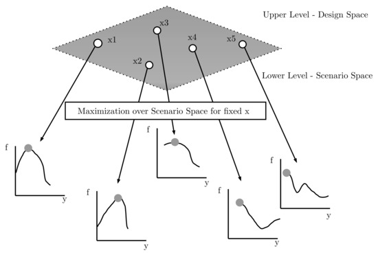
Figure 1.
A general sketch of the min-max optimization problem as a bilevel problem, inspired by [16].
When the problem holds the following condition:
then the problem is symmetrical. Problems that satisfy the symmetrical condition are simpler to solve since the feasible regions of the upper and lower level are independent.
3. Algorithm Method
In this section, we briefly describe the differential evolution and estimation of distribution algorithms. Then, we explain the proposed algorithm for obtaining worst-case scenario optimization.
3.1. Differential Evolution (DE)
DE [17] is a population-based metaheuristic search algorithm and falls under the category of evolutionary algorithm methods. Following the standard schema of such methods, it is based on an evolutionary process, where a population of candidate solutions goes through mutation, crossover, and selection operations. The main steps of the algorithm can be seen below:
- 1.
- Initialization: A population of individuals is randomly initialized. Each individual is represented by a D dimensional parameter vector, where , , where is the maximum number of generations. Each vector component is subject to upper and lower bounds and . The initial values of the ith individual are generated as:where rand(0,1) is a random integer between 0 and 1.
- 2.
- Mutation: The new individual is generated by adding the weighted difference vector between two randomly selected population members to a third member. This process is expressed as:V is the mutant vector, X is an individual, are randomly chosen integers within the range of and , G corresponds to the current generation, F is the scale factor, usually a positive real number between 0.2 and 0.8. F controls the rate at which the population evolves.
- 3.
- Crossover: After mutation, the binomial crossover operation is applied. The mutant individual is recombined with the parent vector , in order to generate the offspring . The vectors of the offspring are inherited from or depending on a parameter called crossover probability, as follows:where is a uniformly generated number, is a randomly chosen index, which assures that gives at least one element to . denotes the t-th element of the individual’s vector.
- 4.
- Selection: The selection operation is a competition between each individual and its offspring and defines which individual will prevail in the next generation. The winner is the one with the best fitness value. The operation is expressed by the following equation:The above steps of mutation, crossover, and selection are repeated for each generation until a certain set of termination criteria has been met. Figure 2 shows the basic flowchart of the DE.
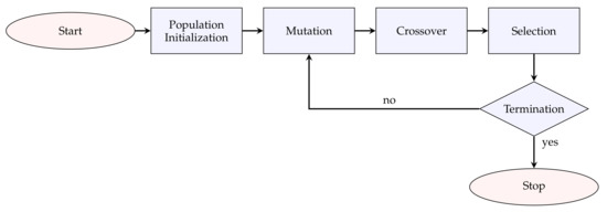 Figure 2. Basic flowchart of the differential evolution algorithm (DE).
3.2. Estimation of Distribution Algorithms (EDAs)
The basic flowchart of the EDA is shown in Figure 3. The general steps of the EDA algorithm are the following:
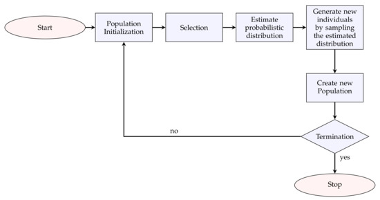
Figure 3.
Basic flowchart of the estimation of distribution algorithm (EDA).
- 1.
- Initialization: A population is initialized randomly.
- 2.
- Selection: The most promising individuals from the population , where t is the current generation, are selected.
- 3.
- Estimation of the probabilistic distribution: A probabilistic model is built from .
- 4.
- Generate new individuals: New candidate solutions are generated by sampling from the .
- 5.
- Create new population: The new solutions are incorporated into , and go to the next generation. The procedure ends when the termination criteria are met.
3.3. Proposed Algorithm
In the proposed algorithm, we keep the hierarchically nested formulation of a min-max problem, which solves asymmetrical problems. The design space (UL) decision variables are evolving with a DE. For the evaluation of each UL individual, first the scenario space (LL) problem is solved by the DE. This solution is then transferred to the upper level. To reduce the cost, we apply an estimation of distribution mechanism between the decision space search (UL) and the scenario space search (LL). In that way, we use a priori knowledge obtained during the optimization. To further reduce the FEs, we search only for solutions with good worst-case scenarios. If the objective function of a solution under any scenario is already worse in terms of worst-case performance of the best solution found so far, there is no need for further exploring over scenario space. Therefore, the mutant individual’s performance is checked under the parent’s worst-case scenario, and further explored only when it is better in terms of the fitness function. Figure 4 shows the general framework of the proposed approach. The main steps of the proposed algorithm for the UL:
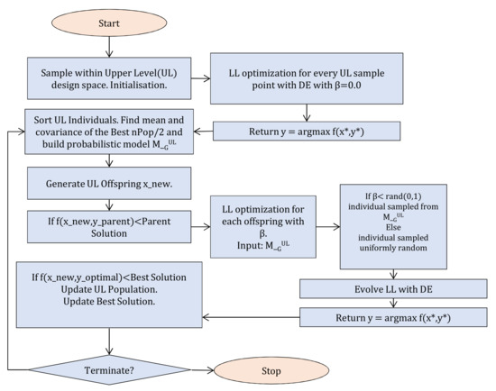
Figure 4.
General framework of the proposed algorithm.
- 1.
- Initialization: A population of size is initialized according to the general DE procedure mentioned in the previous section, where the individuals are representing candidate solutions in the design space X.
- 2.
- Evaluation: To evaluate the fitness function, we need to solve the problem in the scenario space. For a fixed candidate UL solution , the LL DE is executed. More detailed steps are given in the next paragraphs. The LL DE returns the solution corresponding to the worst-case scenario for the specific . For each individual, the corresponding best solutions are stored, meaning the solution y that for a fixed x maximizes the objective function.
- 3.
- Building: The individuals in the population are sorted as the ascending of the UL fitness values. The best are selected. From the best individuals, we build the distribution to establish a probabilistic model for the LL solution. The d-dimensional multivariate normal densities to factorize the joint probability density function (pdf) are:where x is the d-dimensional random vector, is the d-dimensional mean vector and is the covariance matrix. The two parameters are estimated from the best of the population, from the stored lower level best solutions. In that way, in each generation, we extract statistical information about the LL solutions of the previous UL population. The parameters are updated accordingly in each generation, following the general schema of an estimation of distribution algorithm.
- 4.
- Evolution: Evolve UL with the steps of the standard DE of mutation, crossover, producing an offspring .
- 5.
- Selection: As mentioned above, the selection operation is a competition between each individual and its offspring . The offspring will be evaluated in the scenario space and sent in LL only if ≤, where corresponds to the worst case vector of the parent individual . In that way, a lot of unneeded LL optimization calls will be avoided, reducing FEs. If the offspring is evaluated in the scenario space, the selection procedure in Equation (6) is applied.
- 6.
- Termination criteria:
- Stop if the maximum number of function evaluations is reached.
- Stop if the improvement of the best objective value of the last generations is below a specific number.
- Stop if the absolute difference of the best and the known true optimal objective value is below a specific number.
- 7.
- Output: the best worst case function value , the solution corresponding to the best worst-case scenario
For the LL:
- 1.
- Setting: Set the parameters of the probability of crossover , the population size , the mutation rate F, the sampling probability .
- 2.
- Initialization: Sample individuals to initialize the population. If , then the individual is sampled from the probabilistic model built in the UL with the Equation (7). The model here is sampled with the built-in function of Matlab, which accepts a mean vector mu and covariance matrix sigma as input and returns a random vector chosen from the multivariate normal distribution with that mean and covariance [23]. Otherwise, it is uniformly sampled in the scenario space according to the Equation (3). Please note that for the first UL generation, is always 0, as no probabilistic model is built yet. For the following generations, can range from (0,1) number, where = 1 means that the population will be sampled only from the probabilistic model. This might lead the algorithm to be stuck in local optima and to converge prematurely. An example of an initial population generated with the aforementioned method with = 0.5 is shown in Figure 5. Magenta asterisk points represent the population generated by the probabilistic model of the previous UL generation. Blue points are samples uniformly distributed in the search space. In Figure 6, the effect of the probabilistic model on the initial population of LL for during the optimization is shown. As the iterations increase, the LL members of the populations sampled from the probabilistic distribution reach the promising area that maximizes the function. In the zoomed subplot in each subfigure, one can see that all such members of the population are close to the global maximum, compared to the randomly distributed members.
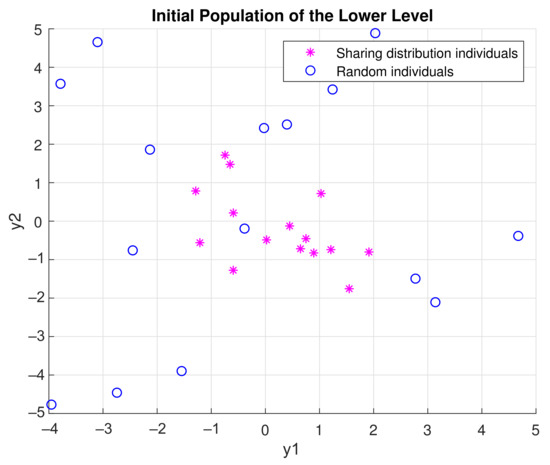 Figure 5. Balancing exploration and exploitation with the sharing distribution mechanism of the LL population. Magenta asterisk points represent the population generated by the distribution of the previous UL generations. Blue points are samples uniformly distributed in the search space. The idea behind this is to keep the “knowledge” already gained in previous generations while also giving the opportunity to the algorithm to search the whole search space. Here with .
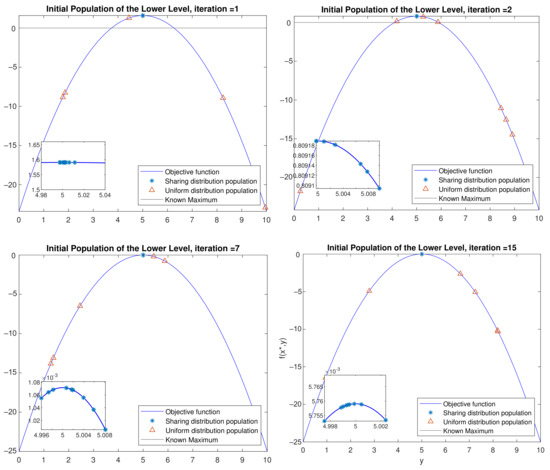 Figure 6. Effect of the probabilistic model on the initial population of LL for . As the iterations increase, the LL members of the population that were produced from the probabilistic model reach the promising area that maximizes the function. The area they are concentrated is shown in the zoomed plots of each plot.
 - 3.
- Mutation, crossover, and selection as the standard DE.
- 4.
- Termination criteria:
- Stop if the maximum number of generations is reached.
- Stop if the absolute difference between the best and the known true optimal objective value is below a specific number.
- 5.
- Output: the maximum function value , the solution corresponding to the worst-case scenario .
4. Experimental Settings
In this section, we describe the 13 benchmark test functions used for this study and provide the parameter settings for our experiments.
4.1. Test Functions
The performance of the proposed algorithm was tested on 13 benchmark problems of min-max optimization. The problems used are found collected in [15] along with their referenced optimal values. The first 7 problems – are taken from [24] and they are convex in UL and concave in the LL. The problems described as min-max are:
Test function :
with . The points and are the known solutions of the , and the optimal value is approximated at .
Test function :
with . The points and are the known solutions of the , and the optimal value is approximated at .
Test function :
with . The points and are the known solutions of the , and the optimal value is approximated at .
Test function :
with , . The points and are the known solutions of the , and the optimal value is approximated at .
Test function :
with , . The points and are the known solutions of the , and the optimal value is approximated at .
Test function :
with , . The points and are the known solutions of the , and the optimal value is approximated at .
Test function :
with . The points and are the known solutions of the , and the optimal value is approximated at .
Test function [25]:
with . The points and are the known solutions of the , and the optimal value is approximated at . This test function is a saddle point function. The function along with the known optimum is plotted in Figure 7, and it serves as an example of a symmetric function.
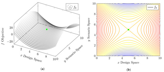
Figure 7.
Three-dimensional mesh and contour plots of the symmetrical test function f8. Green dot corresponds to the known optimum. (a) A 3D mesh of the symmetrical test function f8. (b) Contour plot of the symmetrical test function f8.
Test function [25]:
with . The points and are the known solutions of the , and the optimal value is approximated at . It is a two-plane asymmetrical function. The contour plot and 3-D plot of this function, along with the known optima, are shown in Figure 8 and serves as an example of an asymmetrical function.
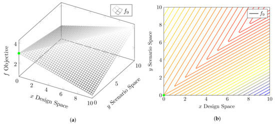
Figure 8.
3D mesh and contour plots of the asymmetrical test function f9. Green dot corresponds to the known optimum. (a) 3D mesh of the asymmetrical test function f9. (b) Contour plot of the asymmetrical test function f9.
Test function [25]:
with . The points and are the known solutions of the , and the optimal value is approximated at . It is a damped sinus asymmetrical function.
Test function [25]:
with . The points and or are the known solutions of the , and the optimal value is approximated at . It is a damped cosine wave asymmetrical function.
Test function [6]:
with . The points and are the known solutions of the , and the optimal value is approximated at .
Test function [6]:
with . The points and are the known solutions of the , and the optimal value is approximated at .
4.2. Parameter Settings
The parameter setting used for all the experiments of this study are shown in Table 1. The population size depends on the dimensionality of the problem, where for the UL is used and for the LL , where is the dimensionality of the UL and LL, respectively.

Table 1.
Control parameters used in the reported results.
All the simulations were undertaken on an Intel (R) Core (TM) i7-7500 CPU @ 2.70 GHz, 16 GB of RAM, and the Windows 10 operating system. The code and the experiments were implemented and run in Matlab R2018b.
5. Experimental Results and Discussion
5.1. Effectiveness of the Probabilistic Sharing Mechanism
To evaluate the effectiveness of the probabilistic sharing mechanism of the proposed algorithm, we compare three different instances that correspond to three different values. The first algorithmic instance has , meaning that the estimation of distribution in the optimization procedure is not activated, and the algorithm becomes a traditional nested DE. This instance serves therefore as the baseline. The second algorithmic instance corresponds to , where half of the initial population of the LL is sampled from the probabilistic model. Last, for the third algorithmic instance, we set a value of , testing the ability of the algorithm when 80% of the initial population of the LL is sampled from the probabilistic model.
Due to the inherent randomness of the EAs, repeated experiments are held to assess a statistical analysis of the performance of the algorithm. We report results of 30 independent runs, which is the minimum number of samples used for statistical assessment and tests. In Table 2, the statistical results of the 30 runs of the different instances of the algorithm are reported. More specifically, we report the mean, median, and standard deviation of the accuracy of the objective function. We calculate the accuracy as the absolute differences between the best objective function values provided by the algorithms and the known global optimal objective values of each test function. This is expressed as
where and are the best and the true optimal values, respectively.
Table 2.
Accuracy comparison of the different instances of the algorithm over the 30 runs.
In order to compare the instances, the non-parametric statistical Wilcoxon signed-rank test [26] was carried out at the 5% significance, where for each test function, the best instance in terms of median accuracy used a control algorithm against the other two. The reported ≤0.05 means that it rejects the null hypothesis and the two samples are different, while >0.05 means the opposite. The best algorithm in terms of median accuracy is shown in bold. We also report the median of the total number of function evaluations. In bold are the lowest median FEs corresponding to the best algorithmic instance in terms of median accuracy. As we can see, the proposed method outperforms the baseline in most of the test functions. More specifically, the second and the third instances are significantly better than the first in the test functions and . For these test functions, the results of these two instances do not differ significantly, therefore there is a tie. What we can note though, is that instance 2 repeatedly requires fewer FEs to reach the same results. Therefore, it performs better in terms of computation expense. For test function , all the instances are performing equally in terms of median accuracy, while the baseline instance reports less FEs. The third instance is best in test functions -. For test function , there is a tie between the second and third instance. The first instance performs better in test functions and , while for , the first and second instance outperforms the third. In many cases, the baseline algorithmic case reports a low number of FEs. These cases, where it does not reach the desired accuracy, indicate premature convergence, when the “least improvement” termination criterion is activated and the algorithm is terminated before reaching the maximum number of evaluations. In 11 out of 13 test functions, instance 2 outperforms at least one instance or performs equally, which makes selecting a a safe choice.
In Figure 9, the success rate of each algorithmic instance and each test function is reported. As a success rate, we define here the percentage of the number of runs where the algorithm reached the desired accuracy of the total runs for each test function. It is interesting to note that the baseline first instance did not at all reach the desired accuracy in 9 out of 13 test problems. The performance of the algorithm improves dramatically by the use of the estimation of distribution. On the other hand, the instance with reaches the desired accuracy for at least one run in 11 out of 13 problems and, instance with in 10 out of 13 problems. The second instance reaches the accuracy of 100% for asymmetrical functions and . For test functions and , none of the algorithms reach the desired accuracy in the predefined number of FEs. is one of the test problems with higher dimensionality, and a higher number of function evaluations might be needed in order to reach higher accuracy.
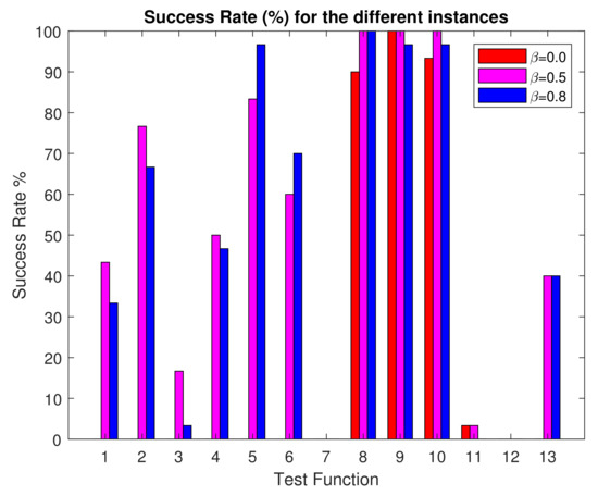
Figure 9.
Barchart of the success rate (%) of each algorithmic instance and each test function. The red color corresponds to the instance where , magenta and blue .
In Figure 10, the convergence plots of the accuracy of the upper level for each algorithmic instance and test function are shown. The red color corresponds to the instance where , magenta and blue . The bumps that can be spotted in the convergence are probably because of inaccurate solutions of the worst-case scenario. This can be mostly seen in Figure 10g, for test function , where the convergence seems to go further than the desired accuracy. In Figure 10j for , algorithmic instance 2 and 3 seem to converge in even earlier generations, in contrast to the baseline first algorithmic instance.
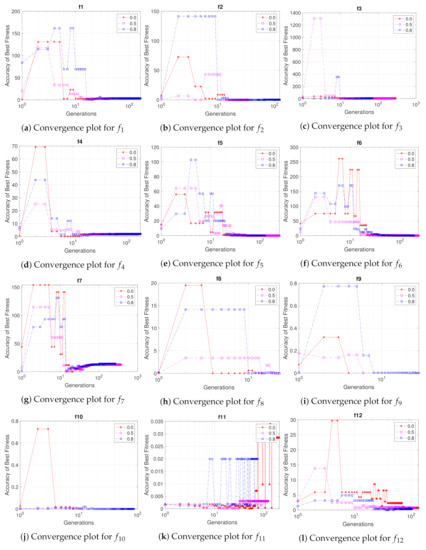
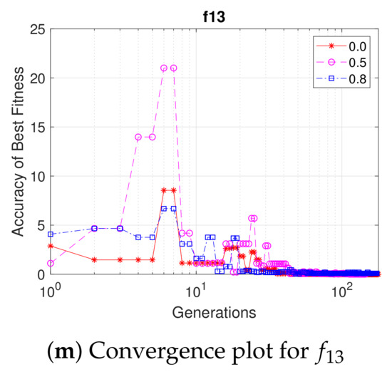
Figure 10.
Fitness accuracy convergence of the upper level of the median run for all the test functions and algorithm instances. The red color corresponds to the instance where , magenta and blue . Generations axes is in logarithmic scale.
5.2. Comparison with State-of-the-Art Method MMDE
In this subsection, we compare the proposed method with one state-of-the-art min-max EA. The MMDE [13] employs a differential evolution algorithm along with a bottom-boosting scheme and a regeneration strategy to detect best worst-case solutions. The MMDE showed statistically significant superior performance against a number of other min-max EAs, so we only compared with the MMDE. For the comparative experiments, the following settings are applied. For the proposed method, the DE parameters of UL are the same as in Table 1, while for the LL, the population size was set to and . For the MMDE, the proposed settings from the reference paper are used and are crossover and mutation . The MMDE also has two parameters and T that control the number of FEs in the bottom-boosting scheme and partial-regeneration strategy. Here, they are set to 190 and 10, respectively, as in the original settings. To have a fair comparison, the termination criterion for both algorithms is only the total number of FEs and set to . Since the number of FEs is limited, an additional check was employed for the proposed method, where if a new solution of the UL is already found in the previous population, then it is not passed to the lower level, since the worst-case scenario is already known. The algorithms are run 30 times on test functions . For comparing the two methods, we use the mean square error (MSE) of the obtained solutions in the design space (UL) to the true optimum, a metric commonly used for comparing min-max algorithms. More specifically, the MSE is calculated:
where is the best solution found by the algorithm and the known optimal solution, while is the dimensionality of the solution. In Table 3, we report the mean, median and standard deviation of the mean square error (MSE). In Figure 11, these values are illustrated as boxplots. The Wilcoxon signed-rank test [26] was conducted at the 5% significance, and we report if the p-value rejects or not the null hypothesis. The proposed method outperforms the MMDE for the test functions and , while it performs equally good on asymmetrical test function . On the test functions –, the MMDE performs better than the proposed method.
Table 3.
MSE Comparison with MMDE over 30 runs and FEs.
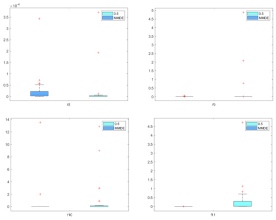
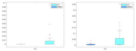
Figure 11.
Boxplots of MSE values of the proposed method and MMDE over 30 runs for the test functions –.
5.3. Engineering Application
To further investigate the performance of the proposed method, we solved a simple engineering application that also serves a benchmark, taken from [27]. It refers to the optimal design of a vibration absorber (Figure 12) for a structure where uncertainties occur in the forcing frequency. A structure with mass is subjected to a force and an unknown frequency. Through a viscous damping effect, a smaller structure of mass is employed to compensate for the oscillations caused by this disturbance. The design challenge is to figure out how to make this damper robust to the worst force frequency. The objective function is the normalized maximum displacement of the main structure and is expressed as [27]:
where
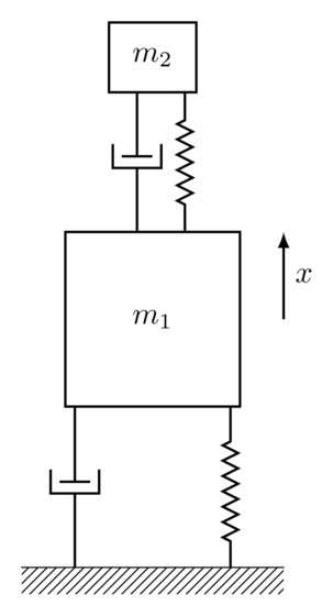
Figure 12.
Vibration absorber.
The fixed parameters for the specific problem are and . The decision variables in the design space are and T, while variable is the decision variable in the scenario space against which the design should be robust against. The problem can be written as a min-max problem:
with , and . The points and are the known solutions of the J, and the optimal value is approximated at as reported in [28]. We run the problem 30 independent times for both the proposed method and the MMDE algorithm with the same parameter settings as in the previous subsection. In Table 4, we report the mean, median and standard deviation of the obtained accuracy and MSE for the proposed method and the MMDE. Both algorithms perform well at approximate the known global optima with an accuracy of ×10 and MSE × 10. The statistical test showed that the proposed method performs equally well with the MMDE for the engineering application.
Table 4.
Statistical comparison with MMDE over 30 runs and FEs for the engineering application.
6. Conclusions
In this work, we propose an algorithm for solving worst-case scenario optimization as a min-max problem. The algorithm employs a nested differential evolution with an estimation of the distribution between the two levels to enhance the efficiency of solving the problems in terms of both accuracy and computational cost. A probabilistic model is built from the best worst-case solutions found so far and is used to generate samples as an initial population of the lower level DE to speed up the convergence. First, the efficiency is investigated by comparing the nested algorithm with different probabilities of using the probabilistic model on 13 test functions of various dimensions and characteristics. To further investigate the performance of the algorithm, it is compared with the MMDE, one state-of-the-art algorithm known to perform well on these problems on both benchmark functions and on an engineering application. The results show that, most times, the proposed method performs better or equal to the MMDE.
In future work, the method could be tested with different population-based EAs in UL or LL, as it is independent of the evolutionary strategy. The parameter, , that defines the probability that the probabilistic model will be used, could be adapted during the optimization. Last, the method can be tested on higher dimensional test functions and/or engineering applications.
Author Contributions
Conceptualization, M.A.; methodology, M.A.; software, M.A.; validation, M.A.; formal analysis, M.A.; investigation, M.A.; writing—original draft preparation, M.A.; writing—review and editing, M.A. and G.P.; visualization, M.A.; supervision, G.P.; project administration, G.P.; funding acquisition, G.P. All authors have read and agreed to the published version of the manuscript.
Funding
This work was supported by the European Commission’s H2020 program under the Marie Skłodowska-Curie grant agreement No. 722734 (UTOPIAE) and by the Slovenian Research Agency (research core funding No. P2-0098).
Data Availability Statement
The code and the related results are available on request from the corresponding author.
Acknowledgments
The authors would like to thank Xin Qiu for providing the source code of the MMDE.
Conflicts of Interest
The authors declare no conflict of interest.
Abbreviations
The following abbreviations are used in this manuscript:
| DE | differential evolution |
| EDA | estimation of distribution algorithm |
| UL | upper level |
| LL | lower level |
| BOP | bilevel optimization problem |
| FEs | function evaluations |
References
- Sinha, A.; Lu, Z.; Deb, K.; Malo, P. Bilevel optimization based on iterative approximation of multiple mappings. J. Heuristics 2017, 26, 1–35. [Google Scholar] [CrossRef] [Green Version]
- Antoniou, M.; Korošec, P. Multilevel Optimisation. Optimization under Uncertainty with Applications to Aerospace Engineering; Springer: Cham, Switzerland, 2021; pp. 307–331. [Google Scholar]
- Feng, Y.; Hongwei, L.; Shuisheng, Z.; Sanyang, L. A smoothing trust-region Newton-CG method for minimax problem. Appl. Math. Comput. 2008, 199, 581–589. [Google Scholar] [CrossRef]
- Montemanni, R.; Gambardella, L.M.; Donati, A.V. A branch and bound algorithm for the robust shortest path problem with interval data. Oper. Res. Lett. 2004, 32, 225–232. [Google Scholar] [CrossRef]
- Aissi, H.; Bazgan, C.; Vanderpooten, D. Min–max and min–max regret versions of combinatorial optimization problems: A survey. Eur. J. Oper. Res. 2009, 197, 427–438. [Google Scholar] [CrossRef] [Green Version]
- Barbosa, H.J. A coevolutionary genetic algorithm for constrained optimization. In Proceedings of the 1999 Congress on Evolutionary Computation-CEC99 (Cat. No. 99TH8406), Washington, DC, USA, 6–9 July 1999; IEEE: Piscataway, NJ, USA; 3, pp. 1605–1611. [Google Scholar]
- Shi, Y.; Krohling, R.A. Co-evolutionary particle swarm optimization to solve min-max problems. In Proceedings of the 2002 Congress on Evolutionary Computation. CEC’02 (Cat. No. 02TH8600), Honolulu, HI, USA, 12–17 May 2002; IEEE: Piscataway, NJ, USA; Volume 2, pp. 1682–1687. [Google Scholar]
- Vasile, M. On the solution of min-max problems in robust optimization. In Proceedings of the EVOLVE 2014 International Conference, A Bridge between Probability, Set Oriented Numerics, and Evolutionary Computing, Beijing, China, 1–4 July 2014. [Google Scholar]
- Chen, R.B.; Chang, S.P.; Wang, W.; Tung, H.C.; Wong, W.K. Minimax optimal designs via particle swarm optimization methods. Stat. Comput. 2015, 25, 975–988. [Google Scholar] [CrossRef]
- Antoniou, M.; Papa, G. Solving min-max optimisation problems by means of bilevel evolutionary algorithms: A preliminary study. In Proceedings of the 2020 Genetic and Evolutionary Computation Conference Companion, Cancun, Mexico, 8–12 July 2020; pp. 187–188. [Google Scholar]
- Angelo, J.S.; Krempser, E.; Barbosa, H.J. Differential evolution for bilevel programming. In Proceedings of the 2013 IEEE Congress on Evolutionary Computation, Cancun, Mexico, 20–23 June 2013; IEEE: Piscataway, NJ, USA; pp. 470–477. [Google Scholar]
- He, X.; Zhou, Y.; Chen, Z. Evolutionary bilevel optimization based on covariance matrix adaptation. IEEE Trans. Evol. Comput. 2018, 23, 258–272. [Google Scholar] [CrossRef]
- Qiu, X.; Xu, J.X.; Xu, Y.; Tan, K.C. A new differential evolution algorithm for minimax optimization in robust design. IEEE Trans. Cybern. 2017, 48, 1355–1368. [Google Scholar] [CrossRef] [PubMed]
- Zhou, A.; Zhang, Q. A surrogate-assisted evolutionary algorithm for minimax optimization. In Proceedings of the IEEE Congress on Evolutionary Computation, Barcelona, Spain, 18–23 July 2010; IEEE: Piscataway, NJ, USA; pp. 1–7. [Google Scholar]
- Marzat, J.; Walter, E.; Piet-Lahanier, H. Worst-case global optimization of black-box functions through Kriging and relaxation. J. Glob. Optim. 2013, 55, 707–727. [Google Scholar] [CrossRef] [Green Version]
- Wang, H.; Feng, L.; Jin, Y.; Doherty, J. Surrogate-Assisted Evolutionary Multitasking for Expensive Minimax Optimization in Multiple Scenarios. IEEE Comput. Intell. Mag. 2021, 16, 34–48. [Google Scholar] [CrossRef]
- Storn, R.; Price, K. Differential evolution–a simple and efficient heuristic for global optimization over continuous spaces. J. Glob. Optim. 1997, 11, 341–359. [Google Scholar] [CrossRef]
- Larranaga, P. A review on estimation of distribution algorithms. In Estimation of Distribution Algorithms; Springer: Boston, MA, USA, 2002; pp. 57–100. [Google Scholar]
- Zhao, F.; Shao, Z.; Wang, J.; Zhang, C. A hybrid differential evolution and estimation of distribution algorithm based on neighbourhood search for job shop scheduling problems. Int. J. Prod. Res. 2016, 54, 1039–1060. [Google Scholar] [CrossRef]
- Hao, R.; Zhang, J.; Xin, B.; Chen, C.; Dou, L. A hybrid differential evolution and estimation of distribution algorithm for the multi-point dynamic aggregation problem. In Proceedings of the Genetic and Evolutionary Computation Conference Companion, Kyoto, Japan, 15–19 July 2018; pp. 251–252. [Google Scholar]
- Wang, G.; Ma, L. The estimation of particle swarm distribution algorithm with sensitivity analysis for solving nonlinear bilevel programming problems. IEEE Access 2020, 8, 137133–137149. [Google Scholar] [CrossRef]
- Gorissen, B.L.; Yanıkoğlu, İ.; den Hertog, D. A practical guide to robust optimization. Omega 2015, 53, 124–137. [Google Scholar] [CrossRef] [Green Version]
- Available online: https://www.mathworks.com/help/stats/mvnrnd.html (accessed on 3 August 2021).
- Rustem, B.; Howe, M. Algorithms for Worst-Case Design and Applications to Risk Management; Princeton University Press: Princeton, NJ, USA, 2009. [Google Scholar]
- Jensen, M.T. A new look at solving minimax problems with coevolutionary genetic algorithms. In Metaheuristics: Computer Decision-Making; Springer: Boston, MA, USA, 2003; pp. 369–384. [Google Scholar]
- Wilcoxon, F. Individual comparisons by ranking methods. Biom. Bull. 1945, 1, 80–83. [Google Scholar] [CrossRef]
- Marzat, J.; Walter, E.; Piet-Lahanier, H. A new expected-improvement algorithm for continuous minimax optimization. J. Glob. Optim. 2016, 64, 785–802. [Google Scholar] [CrossRef]
- Brown, B.; Singh, T. Minimax design of vibration absorbers for linear damped systems. J. Sound Vib. 2011, 330, 2437–2448. [Google Scholar] [CrossRef]
Publisher’s Note: MDPI stays neutral with regard to jurisdictional claims in published maps and institutional affiliations. |
© 2021 by the authors. Licensee MDPI, Basel, Switzerland. This article is an open access article distributed under the terms and conditions of the Creative Commons Attribution (CC BY) license (https://creativecommons.org/licenses/by/4.0/).