Abstract
This paper presents a novel method for multi-objective optimisation under uncertainty developed to study a range of mission trade-offs, and the impact of uncertainties on the evaluation of launch system mission designs. A memetic multi-objective optimisation algorithm, named MODHOC, which combines the Direct Finite Elements in Time transcription method with Multi Agent Collaborative Search, is extended to account for model uncertainties. An Unscented Transformation is used to capture the first two statistical moments of the quantities of interest. A quantification model of the uncertainty was developed for the atmospheric model parameters. An optimisation under uncertainty was run for the design of descent trajectories for a spaceplane-based two-stage launch system.
1. Introduction
This paper presents a novel method for multi-objective optimisation under uncertainty, developed to study a range of mission trade-offs and the impact of uncertainties on system models for space launch systems. This is applied to the analysis and design of descent trajectories for a two-stage, partially re-usable launch system based on the Orbital-500R, a commercial system developed by Orbital Access Ltd. (Prestwick, UK) [1]. The set of Pareto-optimal solutions show the trade-off between minimising the induced acceleration limits and maximising the robustness of the solutions by minimising the sensitivity to uncertainties.
Uncertainty quantification (UQ), the science of quantifying the uncertainty in the desired performance of a system, can be a key step in analysing the robustness of a control solution and of the whole guidance, navigation and control chain. Common approaches to UQ use extensive Monte Carlo simulations to account for errors, unmodelled components and disturbances. At a system level, UQ analysis can translate into the assessment of the reliability of the system as a whole, or only of one or more components. An uncertainty quantification analysis is, therefore, a fundamental step towards de-risking any technological solution as it provides a quantification of the variation in performance and probability of recoverable or unrecoverable system failures, given existing information.
The goal here is, therefore, to design a robust guidance trajectory considering the uncertainty related to the atmospheric model which in turn affects the aero-, aerothermal and flight dynamics.
The trajectories are designed using a MODHOC (Multi-Objective Direct Hybrid Optimal Control) solver [2,3]. MODHOC, first developed in collaboration with ESA, is based on a transcription using temporal finite elements (DFET, Direct Finite Elements in Time) of the optimal control problem and a solution of the transcribed problem with a multi-agent multi-objective optimisation algorithm (MACS, Multi-Agent Collaborative Search).
This paper presents an extension of the multi-objective optimal control to account for uncertainties. The extension is based on an unscented transformation to capture the first two statistical moments of the quantities of interest. The result is an unscented multi-objective optimal control approach that can efficiently handle the level of uncertainty in model parameters.
Ross et al. [4] introduced unscented optimal control as the combination of the unscented transform by Julier and Uhlmann [5] combined with deterministic optimal control theory to directly manage uncertainties within an open-loop control framework. This has been applied to single objective optimisation problems mainly in the field of guidance and attitude control [6,7], using pseudospectral optimal control methods [8] with the common Legendre and Chebyhsev polynomials as the bases. Ross et al. [9] later extended the work to account for path constraints on the states and controls. This paper builds on this work by adapting and applying it to a multi-objective optimal control problem, subject to nonlinear boundary and path constraints. The transcription method here uses finite elements on a temporal basis, using Bernstein polynomials, which have been mathematically shown to ensure both the states and controls representations remains feasible over the entire time domain, not just at collocation nodes [10].
The methods presented will be applied to trade-off studies on the first stage of a multi-stage horizontal take-off and landing launch system. The analysis focuses on the unpowered descent trajectory of a spaceplane, starting from the stage separation point at 100 km altitude. Uncertainties are introduced on the atmospheric parameters, which in turn strongly affect the aerodynamics and flight performance of the vehicle. The optimisation will trade-off robustness, by minimising the effect of these uncertainties, against the structural loads induced by the flight dynamics.
The paper is structured first introducing the mathematical method and implementation, followed by the description of the applied test case and results. Specifically, Section 2 describes the integration of an unscented transform into a multi-objective optimal control problem, including the direct transcription method using temporal finite elements with Bernstein bases. Section 3 details the solution of the multi-objective nonlinear programming problem through an adaption of a global evolutionary Multi-Agent Collaborative Search (MACS) algorithm tailored to optimal control problems. Section 4 presents the quantification of the uncertainty on the atmospheric parameters predicted by the International and US-76 Standard Atmospheric models. Section 5 describes the vehicle and environment models for the launch vehicle test case, with Section 6 presenting and discussing the results, including a validation of the methods and results against a Monte Carlo analysis.
2. Unscented Multi-Objective Optimal Control
In order to perform robust optimisation of the trajectory, an Unscented Transformation [5] was included in the formulation of the optimal control problem. An unscented transformation is defined as “the application of a given nonlinear transformation to a discrete distribution of points, computed so as to capture a set of known statistics of an unknown distribution, is referred to as an unscented transformation” [11]. These points are referred to as sigma points.
Unscented transformations capture the first statistical moments, mean and covariance, of the distributions of the states of a system subject to uncertainty and undergoing arbitrary nonlinear transformations by propagating a small number of sigma points. If the system depends on uncertain variables, whose mean and covariances are known, the unscented transformation requires the propagation of samples. The first sigma point takes the mean value for all the uncertain variables, while the others assume the mean plus (or minus) the square root of the matrix of the covariances of the uncertain variables. All the sigma points are propagated simultaneously with the mean and covariance of the final states computed as a weighted combination of the final states of each sigma point.
Let the dynamics of the system be given by
where is the system state vector, are the controls, t is time, and are additional static (time independent) parameters. Similar to (1), the dynamics of each sigma point are given by
where . Each sigma point has a different value for the static variables, its dynamics evolve independently of the other sigma points, but all sigma points are controlled by the same control law . The goal is to find a single control law that, when applied to all sigma points, allows the system to reach a desired final condition and to be optimal, in some sense. The particular values for each static variable is decided by the application of the Unscented Transformation.
A known problem of the unscented transformation is that it can generate covariance matrices that are not semidefinite positive. To avoid this problem, the Square Root Unscented Transformation [12] was implemented. Algorithmically, it is very similar to the standard Unscented Transformation but differs in the way the samples are generated and has the advantage that the resulting covariance matrix is guaranteed to be semidefinite positive (up to machine precision). The sigma points are computed from the Cholesky factorisation of the covariance matrix, which decomposes the matrix into lower triangular matrix with real and positive diagonal entries, and its conjugate transpose [12].
The problem can be described as follows. Let be a state vector of length defined as
where is the number of sigma points and is the number of states of the system. The state dynamics are then defined as
The multi-objective unscented optimal control problem is then formulated as
where is, in general, a vector function of the state variables , control variables and time t. Functions belong to the Sobolev space , objective functions are , , algebraic constraint function , and boundary condition functions .
Direct Transcription with Temporal Finite Elements
The optimal control problem in (5)–(8) is transcribed into a many-objective, nonlinear programming problem via Direct Transcription with Finite Elements in Time (DFET) [13]. DFET was first proposed by Vasile [14] in 2000, and uses finite elements in time on spectral bases to transcribe the differential and algebraic constraints, and objective function into a set of algebraic equations. The formation allows different bases to be selected for both the states and controls, and for different segments. As a scheme, DFET has been proven to be robust, accurate and flexible [13].
For the continuous optimal control problem in (5), the time domain is decomposed into N finite elements , with each element normalised to the interval through the transformation
This ensures the domain of the basis functions are consistent irrespective of the element size. The differential constraints in (6) are first recast in weak variation form as
where are generalised weight functions, and and are the values of the states at the boundaries of each element. For each element , the states, controls, and weight functions can be parameterised according to the basis functions such that:
For this paper, Bernstein polynomials are used as the bases functions for all the elements, of order for the states, for the controls and for the weights. Bernstein basis polynomials are defined generally as
where n is the order. Bernstein bases have the advantage of smooth control profiles with no oscillations near discontinuities or step changes, meaning the polynomial representation of both states and controls remains within the feasible set [10,15].
Recasting (10) into Gauss quadrature using the polynomials in (11)–(13) gives
where and are Gauss nodes and weights, respectively, and is the shorthand notation for . Since (15) must be valid for every arbitrary , this can be written as a system of equations for each element:
The path constraints from (7) are directly collocated at the Gauss nodes, generating a set of constraint equations for each element given by
Constraints are also imposed on the boundary states of all adjacent elements to ensure continuity.
The transcribed objective functions from (5) are therefore
which equate to the two terms in a Bolza optimisation problem [16].
The time domain corresponds to a single time period . For launch systems, however, trajectories often have multiple phases either in series, or in parallel. For example, a multi-stage vehicle can have one phase per vehicle stage with all phases connected in series for the ascent, and/or branching parallel phases for the upper stage ascent, and first stage descent and landing. For a problem with distinct phases, the dynamic constraints (15), path constraints (19), boundary constraints (8) and objective functions (20) are defined per phase. An additional set of boundary constraints are introduced to manage the connections between phases defined by
where the index vector collects all the indexes of the phases that are connected by the constraint . Note that, while the number of phases is fixed, their temporal order is defined by the phase boundary constraints (21).
The resulting multi-objective nonlinear programming (MONLP) problem coming from the transcription of (5)–(8), with the inclusion of phase constraints (21), is given by
where , Y is a box in with , is a solution, or decision, vector that collects all the static and discretised control variables with , with (assuming that each element has the same number of control parameters) and , and collects all path and boundary constraints.
Similar to (5), the solution of (22) is a subset that satisfies the constraints and contains solution vectors that are Pareto efficient. Given the subset of feasible solution vectors, a solution vector is said to be Pareto efficient if , . The symbol of dominance ≻ indicates that, if , then for and such that . In other words, a solution is non-dominated if the values of any of the objective functions, using that solution, cannot be improved without sacrificing at least one of the other objectives [17]. For continuous functions, the subset is a manifold in with dimension [18]. In the following, the goal is to identify a pre-defined countable number of Pareto-efficient solutions contained in .
3. Solution of the Transcribed Problem
The MONLP problem in (22) is solved with an adaption of the Multi-Agent Collaborative Search (MACS) tailored to optimal control problems [10]. MACSoc combines the stochastic agent-based global search in MACS [19,20] with a local refinement of the solutions [21,22] (see Algorithm 1).
| Algorithm 1 MACS optimal control (MACSoc) |
|
At the start of MACSoc, an initial population is generated with agents representing feasible candidate solutions. Next, a set of uniformly spread weight vectors are generated. Each agent is associated with a different weight vector, allowing the agent to converge to a different part of the Pareto-optimal set (set of non-dominated solutions for the multi-objective optimisation problem).
The global search generates candidate solutions for the decision vector using a combination of social and individualistic actions (lines 4 and 7 in Algorithm 1). Each action generates a candidate decision vector, starting from the current solution allocated to a given agent j, and submits it to a bi-level optimisation problem, where the inner level makes the candidate decision vector feasible with respect to constraints, and the outer level assesses whether the solution of the inner level represents an improvement with respect to the current solution allocated to agent j. All feasible and non-dominated solutions are added to the current population , and saved in an archive (lines 5, 6, 8, 9 and 13 in Algorithm 1). A local refinement is triggered periodically after a user-defined number of iterations, and at the end of the algorithm, which update the current population and archive (lines 10–17 in Algorithm 1). The local refinement solves a single level scalarised version of (22).
The entire process alternates between social and individualistic actions, with periodic local refinement, until a maximum number of calls to the objective vector max_fun_eval is reached.
3.1. Bi-Level Global Optimisation Problem
The NLP problem for the global optimisation is defined by
and represents two optimisation sub-problems at two different levels. The outer level minimises the objective function vector and generates a first set of candidate solutions . The inner level looks for state and control vectors that satisfy the constraint functions , and minimise a cost function based on the candidate solutions of the outer loop that look the closest feasible solution to the candidate solution provided by the outer loop. The feasible solution is then passed back to the outer loop to evaluate the objective functions with . The inner level problem is solved with a local, gradient-based optimiser such as SQP or interior point.
In order to reduce the number of iterations required by the inner level to converge, the outer level stores the feasible states from one iteration to be used as a first guess for the inner level at the next iteration. As shown in Figure 1, the feasible states are preserved from iteration k to iteration ; therefore, the outer level only generates candidate solutions for . Thus, for iteration , the inner level is given as initial guesses for states and controls. Despite being associated with , it has been shown to work well as an initial guess also when associated with .
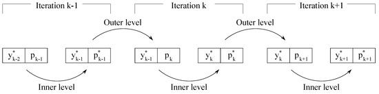
Figure 1.
Schematic representation of the bilevel approach acting on a single solution.
When individualistic actions are applied, each agent generates one or more candidate solution vectors through three mechanisms that are triggered sequentially in the order: Inertia → Pattern Search → Differential Evolution. If any of these mechanisms produces an improved solution, the process is stopped and proceeds to update the population and archive (line 5 and 6 of Algorithm 1).
- Inertia is triggered by agent j only if, in the previous iteration, agent j generated an improved solution. In this case, a step with random length is taken in the direction defined by .
- Pattern Search will change one optimisation parameter at a time, by a random amount in each direction, within a given neighbourhood of agent j. The order by which the parameters are changed is a random permutation of the number of decision parameters. The process is repeated until either an improvement is registered or the maximum number of trials has been reached. As in Ricciardi and Vasile [20], the maximum number of trials is dynamically adjusted during the optimisation process: when the archive is empty, the maximum number of parameters scanned is equal to the total number of optimisation parameters. This maximum value is decreased linearly as the archive fills up, until only one optimisation parameter is changed when the archive is full. The neighbourhood is a box centred in the position of the agent in parameter space and with the edges equal to the edges of the search space multiplied by the scaling parameter .
- Differential Evolution generates a sample with the simple heuristic:where is the current candidate solution, are three randomly chosen solutions from the current population , is a uniformly distributed random number in the unit interval, is a user-defined constant and is a mask vector defined aswhere is another uniformly distributed random number in the unit interval, and is the crossover rate. For the following test cases, and .
If no improvement is made after trying all the three heuristics, ; if instead an improvement is made, until the initial value is reached again.
When social actions are applied, the outer level uses the population to generate a candidate solution using the same heuristics of Differential Evolution (24), with the parent solutions chosen from the union of the current population and the current archive .
A candidate solution generated by the inner level is evaluated in the outer level by computing the weighted Chebychev norm
where is the weight vector in objective space and is the current utopia point.
Given the value of at step k, or , an improvement corresponds to . This improvement criterion has two very important properties: first, it allows the search to reach even non-convex parts of the Pareto front, and, second, if the weights are chosen appropriately, it enables an efficient convergence to the global minimum for each objective function.
Note that, if the inner level does not converge to the required tolerance, the objective functions of the outer level are recalculated to be the infinity norm of the constraint violation plus the maximum values of each objective functions in the archive and population. This creates an adaptive rejection mechanism: if none of the agents are feasible, the ones that best satisfy the feasibility are entered in the archive, with the next iterations trying to improve their feasibility. Once an agent finds a feasible solution, it will explore the search space through the global bi-level approach, generating several feasible and non-dominated solutions. These solutions will enter in the archive as they will dominate many of the existing infeasible solutions, and due to the social actions, some agents will be directly moved onto those solutions, allowing the entire population to converge to feasible solutions in a handful of iterations.
Finally, if any candidate solutions for and fall outside the boundaries of the search space , the solution vector is reduced until it is back within the search space.
3.2. Single Level Local Search
The local refinement solves the following scalarised problem for each agent j:
where is the i component of the weights for the j agent, is the i component of the rescaled objective vector of the j agent, and is a slack variable.
This reformulation of the problem, which uses Pascoletti–Serafini scalarisation [23], constrains the movement of the agent to within a descent cone defined by the point and along the direction . The rescaled vector of the objective functions is therefore
where is equal to , is the initial guess for the solution of (27), and where is the nadir of the archive. The components of the vector are derived from the normalisation
This allows the components of to have values of 1 at the beginning of the local search, and 0 if the agent converges to the target point . Thus, the single level approach avoids biases when the objectives have significantly different scales.
The weighted Chebychev norm in (26) and (27) are equivalent and lead to the same optimal solution if the target point for the Pascoletti–Serafini scalarisation coincides with the utopia point, and the weight vectors are the same [24]. By combining (26) in the global search phase with (27) in the refinement phase, the algorithm ensures a smooth transition from global exploration of the Pareto set, to local convergence.
3.3. Archiving Strategy
MACSoc, through MACS, employs an archiving strategy described in Ricciardi and Vasile [20]. When the elements in the archive are less than the maximum allowed cardinality of , every new feasible and non-dominated solution is recorded in the archive. Once the defined maximum size for the archive is reached, new elements are added to only if they minimise the potential function,
where is the number of elements in the archive .
To avoid biasing in the rejection–retention process when the objectives have different scales, the objective values of the set of non-dominated solutions are all normalised between 0 and 1. This leads to a combinatorial problem that can be solved approximately but efficiently and returns a uniformly spread set of points [20].
3.4. Generation of the Initial Feasible Population
Before the optimisation starts, MACSoc generates an initial population of agents representing feasible candidate solutions.
A first guess for the candidate solutions is generated using Latin Hypercube sampling within the given boundaries, which gives a near-random sample of parameter values from a multidimensional distribution [18]. State variables for each phase are initialised with a linear interpolation between initial and final conditions. For each phase, each equation in (15) is optimised using the inner level subproblem (23) to ensure feasibility through a local gradient-based optimiser. Additional constraints within the phase are then added in, and the problem is re-optimised. Lastly, the linking constraints between phases are then included, and the full resulting problem is optimised for a final time (always using a local optimiser with the inner level objective function in (23)). If at the end of the initialisation phase, an agent is associated with a solution that is not feasible within the prescribed tolerance, that solution is still included in the initial population and submitted to the subsequent optimisation cycle.
For the test case, the tolerance on feasibility is set to , both for the initial population generation, and for determining feasibility within loop. By default, the maximum number of calls to the constraint function is set equal to . An interior point NLP solver was used as it delivered a more robust and consistent convergence to feasible solutions.
3.5. Definition of the Descent Directions and Target Points
The weight vectors for the bi-level global search are generated as follows: first, a simplex in objective space is generated through simplex lattice design [25]. Then, the points of this simplex lattice are projected on the unit sphere by dividing their position vectors by their distance to the origin. This gives a fairly uniform distribution of weight vectors (and thus descent directions) in any dimensional space.
In order to generate a more uniform distribution, however, these weight vectors are refined using a local optimisation of the same potential function E given in (30),
While this approach is valid for general m-objective problems, for two objectives, it is simpler and faster to generate uniform angularly spaced weight vectors. In the following, and each agent is associated with the closest descent direction in criteria space, at the initialisation stage, with the constraint that no two agents can have the same descent direction.
For the single level approach, the weight vectors are allocated to all agents except to those m agents that minimise each individual objective function. For these m agents, the weight vectors are with . These weights are orthogonal because they correspond to the m orthogonal directions in criteria space. If agent j associated with weight does not generate any improvement after two iterations, a new random orthogonal weight is associated with j and (27) is solved with the added constraints,
The reason for the different choice of weight vectors between the bi-level and the single level formulation can be explained as follows: the bi-level formulation explores globally the search space with a population of agents, thus there is the need to maximise the spreading of the solutions; on the contrary, the single-level is used to improve the local convergence of each agent in a normalised criteria space. Thus, the goal of the single level is to return dominating solutions without altering too much their spreading in criteria space.
4. Uncertainty Model for Atmospheric Parameters
Preliminary design and trade-off studies, in particular those employing computationally intensive multidisciplinary design and multi-objective optimisations, typically use global static atmospheric models such as US-76 Standard Atmospheric model, or the International Standard Atmospheric (ISA) model. These models predict the atmospheric pressure p, temperature T and density as function solely of altitude, and employ simplified algebraic expressions for the different atmospheric layers. The models are based on average values for year-round, mid-latitude conditions with moderate solar activity. The ISA is valid up to an altitude above mean sea level of 86 km, while US-76 has an extension up to 1000 km. Due to this, US-76 is often preferred in the field of space launchers over ISA. These two models rely on similar assumptions and methodologies, differing only in the prediction of the temperature in the upper atmosphere (above 32 km).
In order to assess the robustness of the mission design against uncertainties in the atmospheric model, a model of the uncertainty was developed using higher fidelity atmospheric models to create a data set. A number of empirical, global reference atmospheric models exist, for example, to analyse the effect of atmospheric drag on satellites. The Committee on Space Research (COSPAR) in their International Reference Atmosphere reports details three of these models [26]: NRLMSISE-00 [27], Jacchia Bowman reference atmospheric model JB2008 [28], and DTM2013 [29].
The NRLMSISE-00 is a model developed by the US Naval Research Laboratory and accounts for geographic, temporal, solar and magnetic effects through inputs for: date, time of day, geodetic altitude from 0 to 1000 km, geodetic latitude and longitude, local apparent solar time, 81-day average of F10.7 solar flux, daily F10.7 solar flux for previous day, and daily magnetic index.
A statistical analysis of the difference in the models was performed treating those all the input parameters save altitude as uncertain. A set of quasi-random samples were generated for the altitude using a low discrepancy Halton sequence [30], with the corresponding values for T, P and computed using the NRLMSISE-00 model for all altitudes in the range between 0 and 100 km. The altitude limit of 100 km was driven by the test case of the descent phase of a first stage, reusuable spaceplane which is designed to operate within this range.
Every sample of the NRLMSISE-00 model was treated as an equivalent static global atmospheric model, and used to compare against the US-76 model. These differences were treated as random fluctuations in order to quantify the uncertainty.
As shown in Figure 2, the means and standard deviations were determined for each of the three atmospheric parameters. It can be observed that, for the temperature, the mean differences, or relative errors, are very low, with a relative error around 5% for altitudes below 80 km. The mean relative errors for pressure and density are also low for relatively low altitudes, but increase at higher altitudes, with the largest bands around 60 km. Above 40 km, the pressure and density have a very low absolute value, so a large relative error still means a low absolute error.
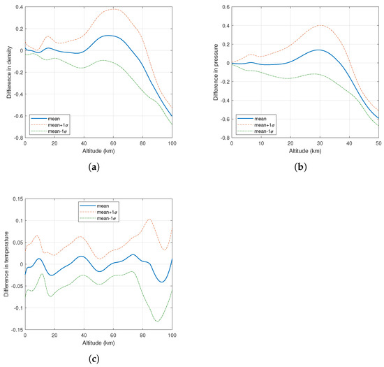
Figure 2.
Mean and standard deviation () of the differences between every sample (representing an equivalent global static atmospheric model) and the US-76 model for each of the atmospheric parameters as a function of altitude. (a) Atmospheric density (kg/m3); (b) Atmospheric pressure (kPa); (c) Atmospheric temperature (K).
Since the approach employed is that of the Square Root Unscented Transformation, different models were generated: one employing the mean relative error, and the others adding to the mean the Cholesky factorisation of the covariance matrix of the uncertain quantities at each altitude. Figure 3 shows the five generated temperature profiles, and their comparison with respect to the US-76 model. A similar approach was followed for the density.
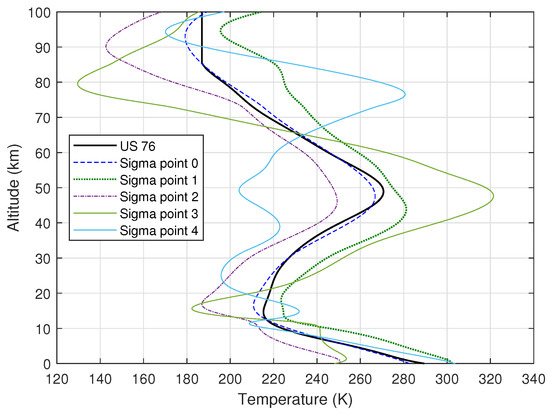
Figure 3.
Temperature profiles for the models of each sigma point, and comparison with the US76 model.
As it can be seen, the Sigma Point 0 model is quite close to the US-76 model. Sigma points 1 and 2 add the standard deviation to this mean, while Sigma points 3 and 4 also include the correlation between variations in temperature and variations in density. The correlation between temperature and density changes sign repeatedly as the altitude changes, thus the profiles assume values lower than one standard deviation only to cross the mean and assume values higher than one standard deviation elsewhere.
Among the samples generated by the Halton sequence on the NRLMSISE-00 model, several profiles do indeed have this kind of shape, which is significantly different to the US-76 model. The temperature affects the computation of the Mach number, on which the aerodynamic coefficients depend. The dependence of the aerodynamic coefficients on the Mach number is stronger around Mach 1 and weaker for high Mach numbers, thus it is not easy to foresee the effect of these variations.
5. Vehicle System Models
The Orbital-500R launch system is composed of a first stage reusable spaceplane, capable of rocket-powered ascent and an unpowered, glided descent, and an expendable, rocket-based upper stage. The system is air-launched from a carrier aircraft. The system was designed to launch from the UK and carry small payloads (500 kg) to Low Earth Orbits (e.g., up to 1500 km). The dry mass of the spaceplane is 20 tonnes.
The flight dynamics are modelled as a variable-mass point with three degrees of freedom in the Earth-centered Earth-fixed reference frame, subject to gravitational, aerodynamic lift and drag forces. The state vector contains the translational position and velocity components, , where is the altitude given radial distance r and the Earth’s radius , are the geodetic latitude and longitude, v is the magnitude of the relative velocity vector directed by the flight path angle and the flight heading angle . The vehicle is controlled through the angle of attack , and the bank angle of the vehicle. The dynamic model is therefore [31]
The Earth is modelled using WSG-84, with gravitational acceleration expressed in radial and tangential components.
The accelerations induced on the vehicle are determined, using the relative vehicle body reference frame .
Surrogate models were used for the lift and drag coefficients as a function of Mach number M, angle of attack and altitude h. An artificial neural network was employed, using an aerodynamic database for the training data coming from a mix of panel methods and CFD simulations (see Stindt et al. [32] for details on the generation of the aerodynamic database). The lift and drag forces were computed assuming no wind, with the relative velocity .
where is the reference area of the vehicle, and is the atmospheric density.
Maddock et al. [1], Ricciardi et al. [10] performed a number trade-off studies through a multi-disciplinary design optimisation on design of the Orbital-500R launch system and on various missions, analysing the full trajectories for both stages. Extrapolating from these results, a nominal starting point for the descent was set. Table 1 lists the initial and final conditions of the state variables. A final condition was imposed on the expected value of the altitude, with a value of 10 km. In addition, the trajectories of all sigma points were required to have a flight path angle greater or equal to .

Table 1.
Values and constraints on the boundary values of the state variables.
6. Application and Results
6.1. Problem Formulation and Set-Up
For the applied test case here, the initial conditions are fixed. The final conditions are affected by the uncertainty, and are expressed as difference between the mean and target values. A boundary constraint is added as follows:
where is the mean of the final states of the sigma points, and is the target value.
The first objective uses a metric to minimise the average induced acceleration on the vehicle. The general formulation is
where the transcribed version using DFET is
where , given in (39)–(41). As part of the generation of the sigma points, weights are generated, associated with each sigma point. The computation of the mean of a quantity, within the transcribed NLP, is the weighted sum of the quantities associated with each sigma point [12].
The second objective aims to reduce the uncertainty of the final state by minimising the sum of the square of all the entries of the covariance matrix:
where is computed using the standard algebraic manipulations employed for the Square Root Unscented transformation, with the additional consideration that no update of the Cholesky factorisation is needed since no measurement is here performed and thus no error is present. This formulation has the advantage that the quantity to compute is smooth and differentiable, it involves all components of the covariance matrix, and does not require iterative procedures like decomposition in eigenvalues to compute the principal axes of the ellipsoid of the uncertainty. In order to give each element of the covariance matrix the same weight even if the quantities of interest have different scales, the state variables were scaled by the same factors internally employed by MODHOC to ensure that all variables assume values between 0 and 1.
The equations were transcribed through DFET, using 6 elements of order 7 for all the states and the controls. Since all five sigma points are propagated simultaneously, there are 30 elements for the states and 12 elements for the controls. MODHOC was run for a total of 30,000 function evaluations, keeping 10 solutions in the archive.
6.2. Trajectory Results
The computed Pareto front is shown in Figure 4, which confirms a trade-off between the two objectives corresponding to metrics to minimising the induced acceleration load on the vehicle (), and maximising the robustness of the trajectory by minimising the covariance of the final values of the state variables ().
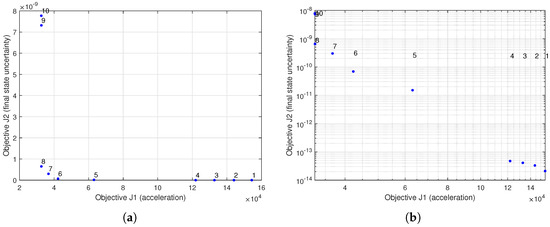
Figure 4.
Pareto Front for the two-objective problem. (a) Linear scale; (b) Log-log scale.
Figure 5 shows the time histories of the state variables for altitude, velocity vector components given by the magnitude, flight path and heading angles. The solutions are shown for a set of Pareto-optimal solutions from Figure 4, along with the uncertainty indicated by the dashed and dotted lines. It can be seen that Solutions 1 to 4 (in greens and blues) have lower uncertainty for the final state, as expected as Solution 1 represents the extrema for . This can also be seen from Figure 6, which show the standard deviation of the same four state variables in Figure 5. As previously stated, even if the uncertainty on atmospheric density is relatively high at high altitudes, its effect is quite limited for the first part of the trajectory as the absolute value is very small (e.g., at 85 km, Pa at 40 km). The uncertainty in the density starts to have a noticeable effect as the altitudes get to approximately 40 and below.
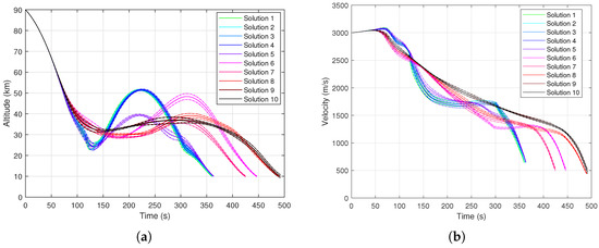
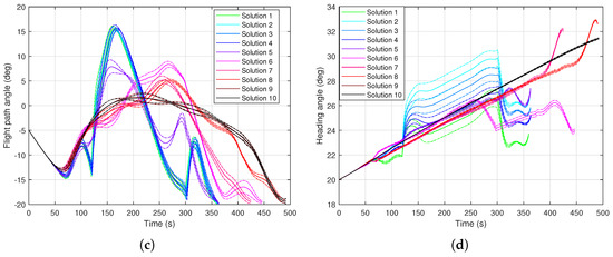
Figure 5.
State variables for set of 10 Pareto-optimal solutions, with dashed and dotted lines showing uncertainty. (a) Altitude; (b) Magnitude of the velocity; (c) Flight path angle; (d) Heading angle.
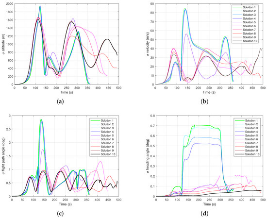
Figure 6.
Standard deviations of state variables. (a) Altitude; (b) Magnitude of velocity; (c) Flight path angle; (d) Heading angle.
As the Pareto front (Figure 4) indicated, the solutions with a lower uncertainty of final states have higher acceleration loads, as shown in Figure 7. This further shows the breakdown between the accelerations in the three vehicle (or body) axes, as well as the magnitude of the acceleration vector.
Figure 7.
Magnitude and components (in vehicle body reference frame) of the induced accelerations, normalised against sea level gravity . (a) Magnitude of acceleration; (b) Component in x-axis; (c) Component in y-axis; (d) Component in z-axis.
Figure 8 shows the time history for the two control variables: angle of attack and bank angle . In all cases, the angle of attack starts with the maximum possible value of , and then progressively decreases to a more moderate value around 5–. Solutions with lower accelerations stay in this regime for a while, and finally conclude with a value around . Solutions with lower final uncertainty instead have a progressive decrease in until small negative values, then a sharp increase to values around 10–, and finally stabilise around .
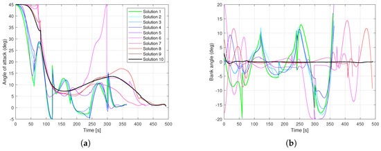
Figure 8.
Control variables, which are consistent across all solutions in the Pareto-optimal set. (a) Angle of attack; (b) Bank attack.
Finally, Figure 9 show the time history of the states for all sigma points for extrema Solutions 1 and 10. As it is evident, the green lines have a much lower scattering at the final time than the black lines, indicating that Solution 1 (green) is subject to less uncertainty than solution 10 (black). These figures also give an idea of the complexity of the problem tackled by this approach, where the same control law is applied to multiple independent sigma points (lines with the same colour) and is able to steer the system to a given expected final state while also reducing the uncertainty associated with the final state, or reducing the expected acceleration load.
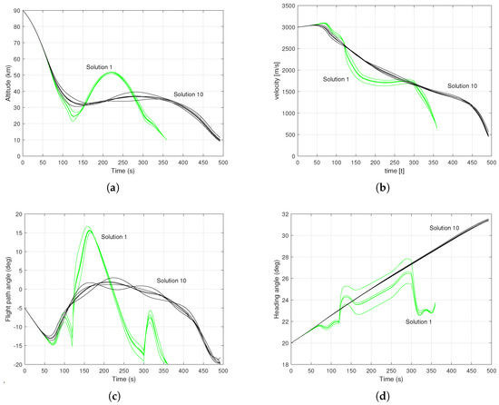
Figure 9.
State variables of sigma points for the two extrema of the Pareto-optimal set (Solutions 1 and 10). (a) Altitude; (b) Velocity; (c) Flight path angle; (d) Heading angle.
6.3. Validation
A Monte Carlo analysis was run to validate the method and results. Starting from the Pareto-optimal set of 10 solutions, the solution was re-integrated using a different sample for the atmospheric model. A 100 different samples (for the atmospheric model) were taken for each Pareto-optimal solution, using the same sampling bounds as used to generate the sigma points (i.e., 1 standard deviation for each of the two atmospheric parameters, density and temperature).
Figure 10 shows the results of the Monte Carlo analysis for a middle set solutions (Solution 7, Figure 10a,b), and the two extrema (Solutions 1 and 10, Figure 10c,d). In each plot, the five sigma points are shown (Point 0 is green, and Points 2–4 in blue), with each of the 100 Monte Carlo runs shown as a grey line.
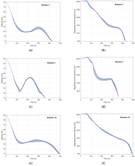
Figure 10.
Monte Carlo analysis for Solution 7 (a,b), Solution 1 (c,d) and Solution 10 (e,f). Green is the central Sigma point 0, blue are Sigma points 1–4, and grey lines are the 100 Monte Carlo samples. (a) Altitude, Solution 7; (b) Velocity, Solution 7; (c) Altitude, Solution 1; (d) Velocity, Solution 1; (e) Altitude, Solution 10; (f) Velocity, Solution 10.
The values of the objective functions are compared in Table 2, looking at the optimised values against the mean values for and across the Monte Carlo runs.
Table 2.
Comparison of the mean value of the objective functions across the 100 runs of the Monte Carlo analysis with the optimised values.
The results from Monte Carlo analysis are consistent with the results found using the unscented transform integrated into the multi-objective optimal control solver MODHOC. Small deviations can be seen towards the middle-end of the trajectory at altitudes below 50 km. The five sigma points chosen are all orthogonal, however the sample points for the Monte Carlo run are not so constrained (though the boundaries are the same). The absolute values for atmospheric parameters, in particular density and pressure p, have higher values in lower atmosphere, so it is consistent with the expectation that this area would experience an increased impact, coupled with the larger standard deviation between 40–60 km.
7. Conclusions
This paper presented an extension of a memetic multi-objective optimisation algorithm MODHOC to perform optimisation under uncertainty. This was applied to a test case to determine a set of Pareto-optimal solutions for the descent trajectory of a first-stage spaceplane, based on the conceptual commercial launch vehicle Orbital 500R. The robust multi-objective optimisation traded off a performance objective, the induced accelerations on the vehicle corresponding to the dynamics loads, with a metric on the robustness of the trajectory to uncertainties on the atmospheric temperature, pressure and density.
Through a square root unscented transformation, different atmospheric models were generated for five sigma points. All the sigma points share the same control law, thus making the trajectory robust against model uncertainty. While only the first two statistical moments of the uncertain values were considered for this work, future work will account for higher order moments, making the resulting trajectory even more robust. A larger number of sigma points will also be required, however, and the resulting optimal control problem becomes progressively larger, requiring the use of large scale optimisation code.
Author Contributions
Conceptualization, L.A.R., C.A.M. and M.V.; Formal analysis, L.A.R., C.A.M. and M.V.; Funding acquisition, C.A.M. and M.V.; Investigation, L.A.R. and C.A.M.; Methodology, M.V.; Project administration, C.A.M., M.V.; Software, L.A.R.; Supervision, C.A.M. and M.V.; Writing—original draft, L.A.R. and C.A.M.; Writing—review & editing, C.A.M. and M.V. All authors have read and agreed to the published version of the manuscript.
Funding
This work has been partially funded by the UK Space Agency and European Space Agency General Support Technology Programme (GSTP) 4000126322/18/NL/LvH/zk on De-risking of the GNC of the Orbital 500-R, and ESA Network Partnership Initiative (NPI) 4000112763/14/NL/GLC/ats on Multi-Objective Hybrid Optimal Control Problems.
Data Availability Statement
The software tools DFET and MACS are available open source under the Strathclyde Mechanical and Aerospace Research Toolbox (SMART) for Optimisation and Optimal Control (o2c) hosted at https://github.com/strath-ace/smart-o2c, accessed on 15 November 2021.
Acknowledgments
The work here uses as a test case a variant of the Orbital-500R launch system that was created and developed by Orbital Access Ltd., and analysed through the Future Space Payload Launcher UK programme which included University of Strathclyde, BAE Systems, Fluid Gravity Engineering Ltd, University of Glasgow and others and was led by Orbital Access Ltd.
Conflicts of Interest
The authors declare no conflict of interest. The funders had no role in the design of the study; in the collection, analyses, or interpretation of data; in the writing of the manuscript, or in the decision to publish the results.
References
- Maddock, C.A.; Ricciardi, L.; West, M.; West, J.; Kontis, K.; Rengarajan, S.; Evans, D.; Milne, A.; McIntyre, S. Conceptual design analysis for a two-stage-to-orbit semi-reusable launch system for small satellites. Acta Astronaut. 2018, 152, 782–792. [Google Scholar] [CrossRef] [Green Version]
- Ricciardi, L.A.; Vasile, M. MODHOC: Multi Objective Direct Hybrid Optimal Control. In Proceedings of the International Conference on Astrodynamics Tools and Techniques, Oberpfaffenhofen, Germany, 6–9 November 2018. [Google Scholar]
- Vasile, M. Multi-objective optimal control: A direct approach. In Satellite Dynamics and Space Missions; Springer: Berlin/Heidelberg, Germany, 2019; pp. 257–289. [Google Scholar] [CrossRef]
- Ross, I.M.; Proulx, R.J.; Karpenko, M. Unscented optimal control for space flight. In Proceedings of the International Symposium on Space Flight Dynamics, Laurel, MD, USA, 5–9 May 2014. [Google Scholar]
- Julier, S.J.; Uhlmann, J.K. A General Method for Approximating Nonlinear Transformations of Probability Distributions; Technical Report; Robotics Research Group, Department of Engineering Science, University of Oxford: Oxford, UK, 1996. [Google Scholar]
- Ross, I.M.; Proulx, R.J.; Karpenko, M.; Gong, Q. Riemann—Stieltjes optimal control problems for uncertain dynamic systems. J. Guid. Control Dyn. 2015, 38, 1251–1263. [Google Scholar] [CrossRef] [Green Version]
- Ozaki, N.; Campagnola, S.; Funase, R.; Yam, C.H. Stochastic differential dynamic programming with unscented transform for low-thrust trajectory design. J. Guid. Control. Dyn. 2018, 41, 377–387. [Google Scholar] [CrossRef]
- Longuski, J.M.; Guzmán, J.J.; Prussing, J.E. Optimal Control with Aerospace Applications; Springer: Berlin/Heidelberg, Germany, 2014. [Google Scholar]
- Ross, I.M.; Karpenko, M.; Proulx, R.J. Path constraints in tychastic and unscented optimal control: Theory, application and experimental results. In Proceedings of the American Control Conference, Boston, MA, USA, 6–8 July 2016. [Google Scholar] [CrossRef]
- Ricciardi, L.A.; Maddock, C.A.; Vasile, M. Direct solution of multi-objective optimal control problems applied to spaceplane mission design. J. Guid. Control Dyn. 2019, 42, 30–46. [Google Scholar] [CrossRef] [Green Version]
- Uhlmann, J.K. Dynamic Map Building and Localisation: New Theoretical Foundations. Ph.D. Thesis, University of Oxford, Oxford, UK, 1995. [Google Scholar]
- Van der Merwe, R.; Wan, E.A. The square-root unscented Kalman filter for state and parameter-estimation. In Proceedings of the IEEE International Conference on Acoustics, Speech and Signal Processing, Salt Lake City, UT, USA, 7–11 May 2001. [Google Scholar] [CrossRef]
- Vasile, M. Finite Elements in Time: A Direct Transcription Method for Optimal Control Problems. In Proceedings of the AIAA/AAS Astrodynamics Specialist Conference, Toronto, ON, Canada, 2–5 August 2010. [Google Scholar] [CrossRef]
- Vasile, M.; Finzi, A. Direct Lunar Descent Optimisation by Finite Elements in Time Approach. Int. J. Mech. Control 2000, 1. [Google Scholar]
- Darehmiraki, M.; Farahi, M.H.; Effati, S. A Novel Method to Solve a Class of Distributed Optimal Control Problems Using Bezier Curves. J. Comput. Nonlinear Dyn. 2016, 11, 061008. [Google Scholar] [CrossRef]
- Betts, J.T. Practical Methods for Optimal Control and Estimation Using Nonlinear Programming; Advances in Design and Control; SIAM: Philadelphia, PA, USA, 2010. [Google Scholar]
- Chankong, V.; Haimes, Y.Y. Multiobjective Decision Making: Theory and Methodology; Courier Dover Publications: Mineola, NY, USA, 2008. [Google Scholar]
- Hillermeier, C. Nonlinear Multiobjective Optimization; International Series of Numerical Mathematics; Birkhäuser Basel: Basel, Switzerland, 2001. [Google Scholar] [CrossRef] [Green Version]
- Zuiani, F.; Kawakatsu, Y.; Vasile, M. Multi-objective optimisation of many-revolution, low-thrust orbit raising for Destiny mission. In Proceedings of the AAS/AIAA Space Flight Mechanics Conference, Kauai, HI, USA, 10–14 February 2013. [Google Scholar]
- Ricciardi, L.A.; Vasile, M. Improved archiving and search strategies for Multi-agent Collaborative Search. In Proceedings of the International Conference on Evolutionary and Deterministic Methods for Design, Optimization and Control with Applications to Industrial and Societal Problems, Glasgow, UK, 14–16 September 2015. [Google Scholar]
- Ricciardi, L.A.; Vasile, M.; Maddock, C. Global solution of multi-objective optimal control problems with Multi Agent Collaborative Search and Direct Finite Elements Transcription. In Proceedings of the IEEE Congress on Evolutionary Computation, Vancouver, BC, Canada, 24–29 July 2016. [Google Scholar] [CrossRef] [Green Version]
- Ricciardi, L.A.; Vasile, M.; Toso, F.; Maddock, C.A. Multi-objective optimal control of the ascent trajectories of launch vehicles. In Proceedings of the AIAA/AAS Astrodynamics Specialist Conference, Napa, CA, USA, 15–18 February 2016. [Google Scholar]
- Pascoletti, A.; Serafini, P. Scalarizing vector optimization problems. J. Optim. Theory Appl. 1984, 42, 499–524. [Google Scholar] [CrossRef]
- Eichfelder, G. Adaptive Scalarization Methods in Multiobjective Optimization; Springer: Berlin/Heidelberg, Germany, 2008. [Google Scholar] [CrossRef]
- Chasalow, S.D.; Brand, R.J. Algorithm AS 299: Generation of Simplex Lattice Points. J. R. Stat. Soc. Ser. C (Appl. Stat.) 1995, 44, 534–545. [Google Scholar] [CrossRef]
- Bruinsma, S.; Arnold, D.; Jäggi, A.; Sánchez-Ortiz, N. Semi-empirical thermosphere model evaluation at low altitude with GOCE densities. J. Space Weather Space Clim. 2017, 7, A4. [Google Scholar] [CrossRef] [Green Version]
- Picone, J.M.; Hedin, A.E.; Drob, D.P.; Aikin, A.C. NRLMSISE-00 empirical model of the atmosphere: Statistical comparisons and scientific issues. J. Geophys. Res. Space Phys. 2002, 107, SIA 15-1–SIA 15-16. [Google Scholar] [CrossRef]
- Bowman, B.; Tobiska, W.K.; Marcos, F.; Huang, C.; Lin, C.; Burke, W. A new empirical thermospheric density model JB2008 using new solar and geomagnetic indices. In Proceedings of the AIAA/AAS Astrodynamics Specialist Conference, Cambridge, MD. USA, 29 June–2 July 2008. [Google Scholar]
- Bruinsma, S. The DTM-2013 thermosphere model. J. Space Weather Space Clim. 2015, 5, A1. [Google Scholar] [CrossRef] [Green Version]
- Niederreiter, H. Random Number Generation and Quasi-MONTE Carlo Methods; SIAM: Philadelphia, PA, USA, 1992. [Google Scholar]
- Zipfel, P. Modeling and Simulation of Aerospace Vehicle Dynamics, Second Edition; AIAA Education Series; AIAA: Reston, VI, USA, 2007. [Google Scholar] [CrossRef]
- Stindt, T.; Merrifield, J.; Fossati, M.; Ricciardi, L.A.; Maddock, C.A.; West, M.; Kontis, K.; Farkin, B.; McIntyre, S. Aerodynamic database development for a future reusable space launch vehicle, the Orbital 500R. In Proceedings of the International Conference on Flight Vehicles, Aerothermodynamics and Re-entry Missions and Engineering, Monopoli, Italy, 30 September–3 October 2019. [Google Scholar]
Publisher’s Note: MDPI stays neutral with regard to jurisdictional claims in published maps and institutional affiliations. |
© 2021 by the authors. Licensee MDPI, Basel, Switzerland. This article is an open access article distributed under the terms and conditions of the Creative Commons Attribution (CC BY) license (https://creativecommons.org/licenses/by/4.0/).