Modified Operators Interpolating at Endpoints

Abstract

Some classical operators (e.g., Bernstein) preserve the affine functions and consequently interpolate at the endpoints. Other classical operators (e.g., Bernstein–Durrmeyer) have been modified in order to preserve the affine functions. We propose a simpler modification with the effect that the new operators interpolate at endpoints although they do not preserve the affine functions. We investigate the properties of these modified operators and obtain results concerning iterates and their limits, Voronovskaja-type results and estimates of several differences.

1. Introduction

Let X be a compact Hausdorff space and $C\left(X\right)$ the space of all real-valued, continuous functions on X, endowed with the usual ordering and the supremum norm. Denote by $\mathbf{1}\in C\left(X\right)$ the function of constant value 1.

Let $S:C\left(X\right)\to C\left(X\right)$ be a Markov operator, i.e., a positive linear operator with $S\mathbf{1}=\mathbf{1}$. Consequently, S is a bounded operator and its norm induced by the supremum norm on $C\left(X\right)$ is equal to 1.

In this paper we are concerned with Markov operators of the form

$${\displaystyle Sf=\sum _{j=0}^s{A}_j\left(f\right)p_j,f\in C\left(X\right),}$$

(1)

where $s\ge 1$, $A_j:C\left(X\right)\to \mathbb{R}$ are positive linear functionals with $A_j\left(\mathbf{1}\right)=1$, and $p_j\in C\left(X\right)$ are linearly independent functions, $p_j\ge 0$, ${\displaystyle \sum _{j=0}^s{p}_j=\mathbf{1}}$.

An essential tool in our study will be the matrix

$$M=\left(\begin{array}{cccc}{A}_0\left(p_0\right)& A_0\left(p_1\right)& \dots & A_0\left(p_s\right)\\ A_1\left(p_0\right)& A_1\left(p_1\right)& \dots & A_1\left(p_s\right)\\ \dots & \dots & \dots & \dots \\ A_s\left(p_0\right)& A_s\left(p_1\right)& \dots & A_s\left(p_s\right)\end{array}\right).$$

(2)

Suppose that there exists $\nu \in \left\{0,1,\dots ,s\right\}$ such that

$$M=\left(\begin{array}{cc}{I}_{\nu \times \nu }& O_{\nu \times (s-\nu +1)}\\ R_{(s-\nu +1)\times \nu }& Q_{(s-\nu +1)\times (s-\nu +1)}\end{array}\right),$$

(3)

where I is the unit matrix, O the null matrix, and all the entries of R and Q are strictly positive.

As shown in [1], the properties of S are strongly influenced by the value of $\nu$. In particular, there are significant differences between the case $\nu =0$ and the cases $\nu >0$.

To illustrate this context, let us present some simple examples. For $n\ge 2$ consider the fundamental Bernstein polynomials

$$p_{n,k}\left(x\right):=\left(\genfrac{}{}{0pt}{}{n}{k}\right)x^k{(1-x)}^{n-k},k\in \{0,1,\dots ,n\},x\in [0,1].$$

The Bernstein, Kantorovich, Durrmeyer, genuine Bernstein-Durrmeyer operators are defined, respectively by:

$$\begin{array}{cc}\hfill B_n(f;x)& {\displaystyle =f\left(0\right)p_{n,0}\left(x\right)+f\left(1\right)p_{n,n}\left(x\right)+\sum _{k=1}^{n-1}f\left({\displaystyle \frac{k}{n}}\right)p_{n,k}\left(x\right),}\hfill \\ \hfill K_n(f;x)& =(n+1)p_{n,0}\left(x\right){\int }_0^{\frac{1}{n+1}}f\left(t\right)dt+(n+1)p_{n,n}\left(x\right){\int }_{\frac{n}{n+1}}^{1}f\left(t\right)dt\hfill \\ \hfill & {\displaystyle +(n+1)\sum _{k=1}^{n-1}{p}_{n,k}\left(x\right){\int }_{\frac{k}{n+1}}^{\frac{k+1}{n+1}}f\left(t\right)dt,}\hfill \\ \hfill D_n(f;x)& =(n+1)p_{n,0}\left(x\right){\int }_0^1{p}_{n,0}\left(t\right)f\left(t\right)dt\hfill \\ \hfill & {\displaystyle +(n+1)p_{n,n}\left(x\right){\int }_0^1{p}_{n,n}\left(t\right)f\left(t\right)dt+(n+1)\sum _{k=1}^{n-1}{p}_{n,k}\left(x\right){\int }_0^1{p}_{n,k}\left(t\right)f\left(t\right)dt,}\hfill \\ \hfill U_n(f;x)& {\displaystyle ={(1-x)}^{n}f\left(0\right)+x^{n}f\left(1\right)+(n-1)\sum _{k=1}^{n-1}\left({\int }_0^{1}f\left(t\right)p_{n-2,k-1}\left(t\right)dt\right)p_{n,k}\left(x\right).}\hfill \end{array}$$

The operators which preserve the affine functions (like $B_n$ and $U_n$) interpolate the function at the endpoints and so $\nu =2$. The aim of this paper is to study a slight modification ${\tilde{L}}_n$ of a given operator $L_n:C[0,1]\to C[0,1]$ (which does not interpolate at endpoints, like Kantorovich or Durrmeyer operators) such that ${\tilde{L}}_n$ interpolates the function at the endpoints and so $\nu =2$, without preserving the affine functions. For example,

$$\begin{array}{cc}\hfill & {\displaystyle {\tilde{K}}_n(f;x):=f\left(0\right)p_{n,0}\left(x\right)+f\left(1\right)p_{n,n}\left(x\right)+(n+1)\sum _{k=1}^{n-1}{p}_{n,k}\left(x\right){\int }_{\frac{k}{n+1}}^{\frac{k+1}{n+1}}f\left(t\right)dt,}\hfill \\ \hfill & {\displaystyle {\tilde{D}}_n(f;x):=f\left(0\right)p_{n,0}\left(x\right)+f\left(1\right)p_{n,n}\left(x\right)+(n+1)\sum _{k=1}^{n-1}{p}_{n,k}\left(x\right){\int }_0^1{p}_{n,k}\left(t\right)f\left(t\right)dt.}\hfill \end{array}$$

Since ${\tilde{L}}_{n}f$ interpolates f at 0 and 1, it provides a better approximation near these endpoints. We will give estimates for ${\tilde{L}}_{n}f-f$ and ${\tilde{L}}_{n}f-L_{n}f$. Using methods from [2,3,4,5,6] we will investigate differences between classical operators and modified operators. General results concerning the iterates and the invariant measures for operators S of the form (1) are given in [1]. In this paper we extend these results in order to cover the case of the modified operators ${\tilde{L}}_n$. As a Markov operator, ${\tilde{L}}_n$ preserves the constant functions; we will identify the other functions fixed by it. They play an essential role in studying the generalized convexity induced by ${\tilde{L}}_n$.

All the above considerations can be extended to the multivariate versions of the operators, defined on the canonical simplex of ${\mathbb{R}}^d$.

2. Limit of Iterates

In this section, we are concerned with the limit of iterates of certain Markov operators.

The next theorem completes and gives another proof of the result contained in Ex. 2.3 [1].

Theorem 1.

Let $\nu =2$. Then, there exists an eigenvector $k={(k_0,k_1,\dots ,k_s)}^t$ of the matrix M, corresponding to the eigenvalue 1, such that k and ${(1,1,\dots ,1)}^t$ are linearly independent. Moreover,

$${\displaystyle \underset{m\to \infty }{lim}{S}^{m}f=A_0\left(f\right)\left({\displaystyle p_0+\sum _{i=2}^s{\displaystyle \frac{k_i-k_1}{k_0-k_1}}{p}_i}\right)+A_1\left(f\right)\left({\displaystyle p_1+\sum _{i=2}^s{\displaystyle \frac{k_0-k_i}{k_0-k_1}}{p}_i}\right),f\in C\left(X\right).}$$

(4)

Proof. 

Due to the structure of the stochastic matrix M, 1 is an eigenvalue having the linearly independent eigenvectors ${(1,1,\dots ,1)}^t$ and k.

As in (2.2) [1], we have for $f\in C\left(X\right)$

$$S^{m}f=(p_0,\dots ,p_s)M^{m-1}{\left(A_0\left(f\right),\dots ,A_s\left(f\right)\right)}^t.$$

(5)

It is known (see [7,8,9]) that

$${\displaystyle B:=\underset{m\to \infty }{lim}{M}^m=\left(\begin{array}{cc}{I}_{2\times 2}& O_{2\times (s-1)}\\ P_{(s-1)\times 2}& O_{(s-1)\times (s-1)}\end{array}\right),}$$

(6)

where P is a matrix of the form

$$P=\left(\begin{array}{cc}{c}_2& 1-c_2\\ \dots & \dots \\ c_s& 1-c_s\end{array}\right),0\le c_j\le 1,j=2,\dots ,s.$$

(7)

Since $Mk=k$, we obtain $M^{m}k=k$ and so $Bk=k$. It follows that $k_0{c}_j+k_1(1-c_j)=k_j$, $j=2,\dots ,s$, i.e., $(k_0-k_1)c_j=k_j-k_1$, $j=2,\dots ,s$. Remark that

$$k_0=k_1\mathrm{implies}{k}_0=k_1=\dots =k_s,$$

(8)

a contradiction with the fact that k and ${(1,1,\dots ,1)}^t$ are linearly independent. Thus,

$$c_j={\displaystyle \frac{k_j-k_1}{k_0-k_1}},j=2,\dots ,s.$$

(9)

From (5) and (6), we infer that

$${\displaystyle \underset{m\to \infty }{lim}{S}^{m}f=(p_0,p_1,\dots ,p_s)B{\left(A_0\left(f\right),\dots ,A_s\left(f\right)\right)}^t.}$$

(10)

Using (9), we obtaim the matrix P and then the matrix B. Now, a straightforward calculation leads to (4) and the proof is finished.  □

Corollary 1.

Let $h:=k_0{p}_0+\dots +k_s{p}_s$, where k is the above eigenvector of M. Then, $Sh=h$.

Proof. 

According to (1),

$$Sh=(p_0,\dots ,p_s){\left(A_0\left(h\right),\dots ,A_s\left(h\right)\right)}^t.$$

(11)

For $j=0,\dots ,s$ one has

$$\begin{array}{cc}\hfill A_j\left(h\right)& =A_j(k_0{p}_0+\dots +k_s{p}_s)=k_0{A}_j\left(p_0\right)+\dots +k_s{A}_j\left(p_s\right)\hfill \\ \hfill & =\left(A_j\left(p_0\right),\dots ,A_j\left(p_s\right)\right)k.\hfill \end{array}$$

This leads to

$${\left(A_0\left(h\right),\dots ,A_s\left(h\right)\right)}^t=Mk=k.$$

Now, (11) implies

$$Sh=(p_0,\dots ,p_s)k=k_0{p}_0+\dots +k_s{p}_s=h,$$

and this concludes the proof.  □

Remark 1.

Let E be the linear subspace generated by 1 and h. Another basis of E is formed by the functions

$${\displaystyle {\phi }_0:=p_0+\sum _{i=2}^s{\displaystyle \frac{k_i-k_1}{k_0-k_1}}{p}_i\mathrm{and}{\phi }_1:=p_1+\sum _{i=2}^s{\displaystyle \frac{k_0-k_i}{k_0-k_1}}{p}_i.}$$

Indeed, ${\phi }_0+{\phi }_1=\mathbf{1}$ and $k_0{\phi }_0+k_1{\phi }_1=h$.

Remark 2.

If $f\in C\left(X\right)$ is fixed by S, then $f\in E$. Indeed, $Sf=f$ implies $S^{m}f=f$ and according to (4) $f=A_0\left(f\right){\phi }_0+A_1\left(f\right){\phi }_1\in E$.

Proposition 1.

(i) $A_i\left(Sf\right)=A_i\left(f\right),f\in C\left(X\right),i=0,1$.

(ii) If $A:C\left(X\right)\to \mathbb{R}$ is a positive linear functional such that $A\left(\mathbf{1}\right)=1$ and $A\left(Sf\right)=A\left(f\right)$, $f\in C\left(X\right)$, then A is a convex combination of $A_0$ and $A_1$.

Proof. 

(i) is a direct consequence of (1), (2) and (3).

(ii) If $A\left(Sf\right)=A\left(f\right)$, $f\in C\left(X\right)$, then $A\left(S^{m}f\right)=A\left(f\right)$, $f\in C\left(X\right)$. As a positive linear functional on $C\left(X\right)$, with $A\left(\mathbf{1}\right)=1$, A is continuous and thus (4) implies

$$A\left(f\right)=A\left(A_0\left(f\right){\phi }_0+A_1\left(f\right){\phi }_1\right),f\in C\left(X\right).$$

Consequently,

$$A\left(f\right)=A_0\left(f\right)A\left({\phi }_0\right)+A_1\left(f\right)A\left({\phi }_1\right),f\in C\left(X\right),$$

(12)

with $A\left({\phi }_0\right)+A\left({\phi }_1\right)=A({\phi }_0+{\phi }_1)=A\left(\mathbf{1}\right)=1$.

Moreover, using (7) and (9), we see that ${\phi }_0\ge 0$ and ${\phi }_1\ge 0$, so that $A\left({\phi }_0\right)\ge 0$, $A\left({\phi }_1\right)\ge 0$.

Now, (12) shows that A is a convex combination of $A_0$ and $A_1$.  □

3. Modified Durrmeyer Operators

For the sake of simplicity, we fix a number $n\ge 3$ and consider the polynomials

$$p_0\left(x\right)={(1-x)}^n,p_1\left(x\right)=x^n,p_j\left(x\right)=\left(\genfrac{}{}{0pt}{}{n}{j-1}\right)x^{j-1}{(1-x)}^{n-j+1},j=2,\dots ,n.$$

The corresponding functionals (see Section 1) will be

$$A_0\left(f\right)=f\left(0\right),A_1\left(f\right)=f\left(1\right),A_k\left(f\right)=(n+1){\int }_0^1{p}_k\left(t\right)f\left(t\right)dt,k=2,\dots ,n.$$

We have

$$\begin{array}{cc}\hfill & A_0\left(p_0\right)=1,A_0\left(p_j\right)=0,j=1,\dots n,\hfill \\ \hfill & A_1\left(p_0\right)=0,A_1\left(p_1\right)=1,A_1\left(p_j\right)=0,j=2,\dots ,n,\hfill \\ \hfill & A_k\left(p_0\right)=\left(\genfrac{}{}{0pt}{}{2n-k+1}{n}\right)/\left(\genfrac{}{}{0pt}{}{2n+1}{n}\right),k=2,\dots ,n,\hfill \\ \hfill & A_k\left(p_1\right)=\left(\genfrac{}{}{0pt}{}{n+k-1}{n}\right)/\left(\genfrac{}{}{0pt}{}{2n+1}{n}\right),k=2,\dots ,n.\hfill \end{array}$$

For $k,j=2,\dots ,n,A_k\left(p_j\right)=\left(\genfrac{}{}{0pt}{}{k+j-2}{k-1}\right)\left(\genfrac{}{}{0pt}{}{2n-k-j+2}{n-k+1}\right)/\left(\genfrac{}{}{0pt}{}{2n+1}{n}\right)$.

Remark that

$$\begin{array}{cc}\hfill & A_k\left(p_j\right)=A_j\left(p_k\right),\hfill \\ \hfill & A_{n-k+2}\left(p_{n-j+2}\right)=A_n\left(p_j\right),k,j=2,\dots ,n,\hfill \end{array}$$

which means that $Q_n$ (see (3) with $s=n$ and $\nu =2$) is symmetric with respect to the main diagonal and the second diagonal.

Moreover,

$$A_k\left(p_0\right)=A_{n-k+2}\left(p_1\right),k=2,\dots ,n,$$

so that $R_n$ is symetric with respect to its center.

Explicitly, the matrix $M_n$ is

$${\displaystyle \frac{1}{\left(\genfrac{}{}{0pt}{}{2n+1}{n}\right)}}\left(\begin{array}{cc}\begin{array}{cc}\left(\genfrac{}{}{0pt}{}{2n+1}{n}\right)& 0\\ 0& \left(\genfrac{}{}{0pt}{}{2n+1}{n}\right)\end{array}& \begin{array}{cccc}0& 0& \dots & 0\\ 0& 0& \dots & 0\end{array}\\ \begin{array}{c}\\ \left(\genfrac{}{}{0pt}{}{2n-1}{n}\right)& \left(\genfrac{}{}{0pt}{}{n+1}{n}\right)\\ \\ \left(\genfrac{}{}{0pt}{}{2n-2}{n}\right)& \left(\genfrac{}{}{0pt}{}{n+2}{n}\right)\\ \\ \dots & \dots \\ \\ \left(\genfrac{}{}{0pt}{}{n+1}{n}\right)& \left(\genfrac{}{}{0pt}{}{2n-1}{n}\right)\end{array}& \begin{array}{c}\\ \left(\genfrac{}{}{0pt}{}{2}{1}\right)\left(\genfrac{}{}{0pt}{}{2n-2}{n-1}\right)& \left(\genfrac{}{}{0pt}{}{3}{1}\right)\left(\genfrac{}{}{0pt}{}{2n-3}{n-1}\right)& \dots & \left(\genfrac{}{}{0pt}{}{n}{1}\right)\left(\genfrac{}{}{0pt}{}{n}{n-1}\right)\\ \\ \left(\genfrac{}{}{0pt}{}{3}{2}\right)\left(\genfrac{}{}{0pt}{}{2n-3}{n-2}\right)& \left(\genfrac{}{}{0pt}{}{4}{2}\right)\left(\genfrac{}{}{0pt}{}{2n-4}{n-2}\right)& \dots & \left(\genfrac{}{}{0pt}{}{n+1}{2}\right)\left(\genfrac{}{}{0pt}{}{n-1}{n-2}\right)\\ \\ \dots & \dots & \dots & \dots \\ \\ \left(\genfrac{}{}{0pt}{}{n}{n-1}\right)\left(\genfrac{}{}{0pt}{}{n}{1}\right)& \left(\genfrac{}{}{0pt}{}{n+1}{n-1}\right)\left(\genfrac{}{}{0pt}{}{n-1}{1}\right)& \dots & \left(\genfrac{}{}{0pt}{}{2n-2}{n-1}\right)\left(\genfrac{}{}{0pt}{}{2}{1}\right)\end{array}\end{array}\right).$$

We need an eigenvector k of $M_n$, associated with the eigenvalue 1 and linearly independent of ${(1,1,\dots ,1)}^t$. Due to the structure of $M_n$, we can choose it of the form $k={(1,0,x_1,\dots ,x_{n-1})}^t$. Due to the symmetries of $Q_n$, $w={(0,1,x_{n-1},\dots ,x_1)}^t$ will be also an eigenvector of $M_n$ associated with 1. Therefore, the sum $k+w={(1,1,x_1+x_{n-1},\dots ,x_{n-1}+x_1,)}^t$ is an eigenvector associated with the eigenvalue 1 and having $k_0=k_1=1$ (see (8)). Therefore, $v+w={(1,1,\dots ,1)}^t$. Consequently,

$$x_i+x_{n-i}=1,i=1,\dots ,n-1.$$

We conclude that

(i)

If $n=2j+1$, then the desired eigenvector k can be choosen as

$$(1,0,x_1,\dots ,x_j,1-x_j,\dots ,1-x_1).$$

Instead of $2j$ unknowns, we have only j unknowns $x_1,\dots ,x_j$.

(ii)

If $n=2j$, k has the form

$$(1,0,x_1,\dots ,x_{j-1},\frac{1}{2},1-x_{j-1},\dots ,1-x_1).$$

Instead of $2j-1$, we have only $j-1$ unknowns.

Example 1.

For $n=2$, we obtain the matrix $M_2=\left(\begin{array}{cc}\begin{array}{cc}1& 0\\ 0& 1\end{array}& \begin{array}{c}0\\ 0\end{array}\\ \begin{array}{c}\\ \frac{3}{10}& \frac{3}{10}\end{array}& \begin{array}{c}\\ \frac{4}{10}\end{array}\end{array}\right)$. The corresponding eigenvector k is $k=(2,0,1)$. According to Corollary 1, ${\tilde{D}}_2$ fixes the function $2p_0+p_2=2-2x$. Since ${\tilde{D}}_2\mathbf{1}=\mathbf{1}$, the fixed functions are 1 and x.

Example 2.

For $n=3$, we obtain the matrix

$$M_3=\left(\begin{array}{cc}\begin{array}{cc}1& 0\\ 0& 1\end{array}& \begin{array}{cc}0& 0\\ 0& 0\end{array}\\ \begin{array}{c}\\ \frac{10}{35}& \frac{4}{35}\\ \\ \frac{4}{35}& \frac{10}{35}\end{array}& \begin{array}{c}\\ \frac{12}{35}& \frac{9}{35}\\ \\ \frac{9}{35}& \frac{12}{35}\end{array}\end{array}\right).$$

The eigenvalues are $1,1,\frac{3}{5},\frac{3}{35}$. The eigenvector $k={(1,0,x,1-x)}^t$ can be determined from

$$\left(\frac{10}{35},\frac{4}{35},-\frac{23}{35},\frac{9}{35}\right){(1,0,x,1-x)}^t=0.$$

We obtain $x={\displaystyle \frac{19}{32}}$ and the eigenvector is ${(32,0,19,13)}^t$. Consequently, the operator ${\tilde{D}}_3$ fixes the function

$$32p_0\left(x\right)+19p_2\left(x\right)+13p_3\left(x\right)=32{(1-x)}^3+57{(1-x)}^{2}x+39(1-x)x^2.$$

According to Theorem 1,

$${\displaystyle \underset{m\to \infty }{lim}{\tilde{D}}_3^{m}f=f\left(0\right)\left[p_0+{\displaystyle \frac{19}{32}}{p}_2+{\displaystyle \frac{13}{32}}{p}_3\right]+f\left(1\right)\left[p_1+{\displaystyle \frac{13}{32}}{p}_2+{\displaystyle \frac{19}{32}}{p}_3\right].}$$

Example 3.

For $n=4$, obtain get the matrix

$$M_4={\displaystyle \frac{1}{126}}\left(\begin{array}{cc}\begin{array}{cc}126& 0\\ 0& 126\end{array}& \begin{array}{ccc}0& 0& 0\\ 0& 0& 0\end{array}\\ \begin{array}{c}\\ 35& 5\\ \\ 15& 15\\ \\ 5& 35\end{array}& \begin{array}{c}\\ 40& 30& 16\\ \\ 30& 36& 30\\ \\ 16& 30& 40\end{array}\end{array}\right).$$

The eigenvector $k={\left(1,0,x,\frac{1}{2},1-x\right)}^t$ can be determined from

$$\left(\frac{35}{126},\frac{5}{126},-{\displaystyle \frac{86}{126}},\frac{30}{126},{\displaystyle \frac{16}{126}}\right){\left(1,0,x,\frac{1}{2},1-x\right)}^t=0.$$

We obtain $x={\displaystyle \frac{11}{17}}$ and the eigenvector is ${(1,0,\frac{11}{17},\frac{1}{2},\frac{6}{17})}^t$. Consequently, the operator ${\tilde{D}}_4$ fixes the function

$$34p_0\left(x\right)+22p_2\left(x\right)+17p_3\left(x\right)+12p_4\left(x\right)$$

$$=34{(1-x)}^4+88{(1-x)}^{3}x+102{(1-x)}^2{x}^2+48(1-x)x^3.$$

According to Theorem 1,

$${\displaystyle \underset{m\to \infty }{lim}{\tilde{D}}_4^{m}f=f\left(0\right)\left[p_0+{\displaystyle \frac{11}{17}}{p}_2+{\displaystyle \frac{1}{2}}{p}_3+{\displaystyle \frac{6}{17}}{p}_4\right]+f\left(1\right)\left[p_1+{\displaystyle \frac{6}{17}}{p}_2+{\displaystyle \frac{1}{2}}{p}_3+{\displaystyle \frac{11}{17}}{p}_4\right].}$$

4. The Linking Operator ${\mathit{H}}_{\mathit{n},\mathit{\rho }}$ and Voronovskaja-Type Results

In [10], Păltănea introduced a class of operators that constitute a link between the genuine Bernstein–Durrmeyer operators and the classical Bernstein operators. In [11], Heilmann and Raşa proposed an explicit representation depending on parameter $\rho \ge 1$, which is a link between Bernstein–Durrmeyer operators (for $\rho =1$) and Kantorovich operators (for $\rho \to \infty$). These operators are defined as follows:

$${\displaystyle H_{n,\rho }(f;x)=(n+1)\sum _{j=0}^n{p}_{n,j}\left(x\right){\int }_0^1\left\{{\displaystyle \sum _{i=0}^{\rho -1}{p}_{n\rho +\rho -1,i+j\rho }\left(t\right)}\right\}f\left(t\right)dt,f\in C[0,1].}$$

Consider the modification of the operators $H_{n,\rho }$ as follows:

$${\displaystyle {\tilde{H}}_{n,\rho }(f;x)=f\left(0\right){(1-x)}^n+f\left(1\right)x^n+(n+1)\sum _{j=1}^{n-1}{p}_{n,j}\left(x\right){\int }_0^1\left\{{\displaystyle \sum _{i=0}^{\rho -1}{p}_{n\rho +\rho -1,i+j\rho }\left(t\right)}\right\}f\left(t\right)dt.}$$

The central moments are important in the Shisha and Mond technique used in approximation by positive linear operators. Next, we compare the moments of classical operators with the moments of modified operators.

Denote

$$\begin{array}{cc}\hfill \mathsf{\Delta }& :=H_{n,\rho }\left({(t-x)}^2;x\right)-{\tilde{H}}_{n,\rho }\left({(t-x)}^2;x\right)\hfill \\ \hfill & =(n+1){(1-x)}^n{S}_1+(n+1)x^n{S}_2-x^2{(1-x)}^n-{(1-x)}^2{x}^n,\hfill \end{array}$$

where

$$\begin{array}{cc}\hfill & {\displaystyle S_1:=\sum _{i=0}^{\rho -1}{\int }_0^1{p}_{n\rho +\rho -1,i}\left(t\right){(t-x)}^{2}dt,}\hfill \\ \hfill & {\displaystyle S_2:=\sum _{i=0}^{\rho -1}{\int }_0^1{p}_{n\rho +\rho -1,i+n\rho }\left(t\right){(x-t)}^{2}dt.}\hfill \end{array}$$

By elementary calculations, we find

$$\begin{array}{cc}\hfill S_1& ={\displaystyle \frac{1}{n+1}}\left[{\displaystyle \frac{(\rho +1)(\rho +2)}{3(n\rho +\rho +1)(n\rho +\rho +2)}}-2x{\displaystyle \frac{\rho +1}{2(n\rho +\rho +1)}}+x^2\right],\hfill \\ \hfill S_2& {\displaystyle =\sum _{i=0}^{\rho -1}{\int }_0^1{p}_{n\rho +\rho -1,i+n\rho }\left(t\right){[(1-t)-(1-x)]}^{2}dt}\hfill \\ \hfill & {\displaystyle =\sum _{i=0}^{\rho -1}{\int }_0^1{p}_{n\rho +\rho -1,\rho -1-i}\left(s\right){[s-(1-x)]}^{2}ds}\hfill \\ \hfill & {\displaystyle =\sum _{i=0}^{\rho -1}{\int }_0^1{p}_{n\rho +\rho -1,j}\left(s\right){[s-(1-x)]}^{2}ds}\hfill \\ \hfill & ={\displaystyle \frac{1}{n+1}}\left[{\displaystyle \frac{(\rho +1)(\rho +2)}{3(n\rho +\rho +1)(n\rho +\rho +2)}}-2(1-x){\displaystyle \frac{\rho +1}{2(n\rho +\rho +1)}}+{(1-x)}^2\right].\hfill \end{array}$$

Therefore,

$$\mathsf{\Delta }={\displaystyle \frac{(\rho +1)(\rho +2)}{3(n\rho +\rho +1)(n\rho +\rho +2)}}\left[{(1-x)}^n+x^n\right]-{\displaystyle \frac{\rho +1}{n\rho +\rho +1}}\left[{(1-x)}^{n}x+x^n(1-x)\right].$$

(13)

With similar calculations,

$$\begin{array}{cc}\hfill {\mathsf{\Delta }}_1& :=H_{n,\rho }(t-x;x)-{\tilde{H}}_{n,\rho }(t-x;x)\hfill \\ \hfill & ={\displaystyle \frac{\rho +1}{2(n\rho +\rho +1)}}\left[{(1-x)}^n-x^n\right].\hfill \end{array}$$

(14)

Figure 1 and Figure 2 illustrate the difference $\mathsf{\Delta }$ for $n=10,\rho =2$ and $n=20$, $\rho =5$. We see that indeed the second central moments of ${\tilde{H}}_{n,\rho }$ are smaller than those of $H_{n,\rho }$ near the endpoints.

From relations (13) and (14), we obtain

$${\displaystyle \underset{n\to \infty }{lim}n\left[H_{n,\rho }\left({(t-x)}^2;x\right)-{\tilde{H}}_{n,\rho }\left({(t-x)}^2;x\right)\right]=0,0\le x\le 1.}$$

(15)

$${\displaystyle \underset{n\to \infty }{lim}n\left[H_{n,\rho }\left((t-x);x\right)-{\tilde{H}}_{n,\rho }\left((t-x);x\right)\right]=\left\{\begin{array}{c}0,0<x<1,\hfill \\ \hfill \\ {\displaystyle \frac{\rho +1}{2\rho }},x=0,\hfill \\ \hfill \\ -{\displaystyle \frac{\rho +1}{2\rho }},x=1.\hfill \end{array}\right.}$$

(16)

Considering $k=1$ in Theorem 10 [12], we obtain

$${\displaystyle \underset{n\to \infty }{lim}n\left(H_{n,\rho }f\left(x\right)-f\left(x\right)\right)={\displaystyle \frac{\rho +1}{2\rho }}\left[x(1-x)f^{\prime \prime }\left(x\right)+(1-2x)f^{\prime }\left(x\right)\right],0\le x\le 1.}$$

(17)

Combining (15)–(17), we estimate

$${\displaystyle \underset{n\to \infty }{lim}n\left({\tilde{H}}_{n,\rho }f\left(x\right)-f\left(x\right)\right)=\left\{\begin{array}{c}{\displaystyle \frac{\rho +1}{2\rho }}\left[x(1-x)f^{\prime \prime }\left(x\right)+(1-2x)f^{\prime }\left(x\right)\right],0<x<1,\hfill \\ \hfill \\ 0,x\in \{0,1\}.\hfill \end{array}\right.}$$

(18)

In the following, we prove the Voronovskaja-type result (18).

Theorem 2.

If $f\in C^2[0,1]$, then

$${\displaystyle \underset{n\to \infty }{lim}n\left({\tilde{H}}_{n,\rho }f\left(x\right)-f\left(x\right)\right)=\left\{\begin{array}{c}{\displaystyle \frac{\rho +1}{2\rho }}\left[x(1-x)f^{\prime \prime }\left(x\right)+(1-2x)f^{\prime }\left(x\right)\right],0<x<1,\hfill \\ \hfill \\ 0,x\in \{0,1\}.\hfill \end{array}\right.}$$

Proof. 

Using Korovkin’s Theorem, we obtain

$${\displaystyle \underset{n\to \infty }{lim}(n+1){\int }_0^1{p}_{n,k}(1-x)f\left(x\right)dx=f\left(1\right).}$$

(19)

For $f\in C^1[0,1]$, we obtain

$$\begin{array}{cc}\hfill & {\displaystyle \underset{n\to \infty }{lim}n\left[(n+1){\int }_0^1{p}_{n,k}(1-x)f\left(x\right)dx-f\left(1\right)\right]}\hfill \\ \hfill & =\underset{n\to \infty }{lim}n\left[(n+1){\int }_0^1{p}_{n,k}(1-x)\left(f\left(x\right)-f\left(1\right)\right)dx\right]\hfill \\ \hfill & =limn(n+1)\left(\genfrac{}{}{0pt}{}{n}{k}\right){\int }_0^1{x}^{n-k}{(1-x)}^k\left(f\left(x\right)-f\left(1\right)\right)dx.\hfill \end{array}$$

Integrating by parts, we obtain

$$\begin{array}{cc}\hfill & {\displaystyle \underset{n\to \infty }{lim}n\left[(n+1){\int }_0^1{p}_{n,k}(1-x)f\left(x\right)dx-f\left(1\right)\right]}\hfill \\ \hfill & {\displaystyle =-\underset{n\to \infty }{lim}n{\int }_0^1{p}_{n+1,k}(1-x)\left[f^{\prime }\left(x\right)+k{\displaystyle \frac{f\left(x\right)-f\left(1\right)}{x-1}}\right]dx.}\hfill \end{array}$$

Applying (19), we find

$$\begin{array}{c}\hfill {\displaystyle \underset{n\to \infty }{lim}n\left[(n+1){\int }_0^1{p}_{n,k}(1-x)f\left(x\right)dx-f\left(1\right)\right]=-(k+1)f^{\prime }\left(1\right).}\end{array}$$

(20)

Setting $g\left(t\right)=f(1-t)$, we obtain $f\left(1\right)=g\left(0\right)$, $f^{\prime }\left(1\right)=-g^{\prime }\left(0\right)$, and the relation (20) becomes

$${\displaystyle \underset{n\to \infty }{lim}(n+1)\left[(n+1){\int }_0^1{p}_{n,k}\left(t\right)g\left(t\right)dt-g\left(0\right)\right]=-(k+1)g^{\prime }\left(0\right).}$$

(21)

In (21), we replace n by $(n+1)\rho -1$ and find the formula

$${\displaystyle \underset{n\to \infty }{lim}(n+1)\rho \left[{\displaystyle (n+1)\rho {\int }_0^1{p}_{(n+1)\rho -1,k}\left(t\right)g\left(t\right)dt-g\left(0\right)}\right]=-(k+1)g^{\prime }\left(0\right).}$$

(22)

Summing up, in (22), for $k=0,\dots ,\rho -1$, one obtains

$${\displaystyle \underset{n\to \infty }{lim}n\left[(n+1){\int }_0^1\sum _{k=0}^{\rho -1}{p}_{(n+1)\rho -1,k}\left(t\right)g\left(t\right)dt-g\left(0\right)\right]=-{\displaystyle \frac{\rho +1}{2\rho }}{g}^{\prime }\left(0\right).}$$

(23)

In a similar way, we find

$${\displaystyle \underset{n\to \infty }{lim}n\left[(n+1){\int }_0^1\sum _{k=0}^{\rho -1}{p}_{(n+1)\rho -1,k+n\rho }\left(t\right)f\left(t\right)dt-f\left(1\right)\right]={\displaystyle \frac{\rho +1}{2\rho }}{f}^{\prime }\left(1\right).}$$

(24)

Therefore,

$$\begin{array}{cc}\hfill & {\displaystyle \underset{n\to \infty }{lim}n\left({\tilde{H}}_{n,\rho }f\left(x\right)-H_{n,\rho }f\left(x\right)\right)}\hfill \\ \hfill & {\displaystyle =\underset{n\to \infty }{lim}\left\{n\left[(n+1){\int }_0^1\sum _{k=0}^{\rho -1}{p}_{(n+1)\rho -1,k}\left(t\right)f\left(t\right)dt-f\left(0\right)\right]{(1-x)}^n\right.}\hfill \\ \hfill & +\left.n\left[(n+1){\int }_0^1\sum _{k=0}^{\rho -1}{p}_{(n+1)\rho -1,k+n\rho }\left(t\right)f\left(t\right)dt-f\left(1\right)\right]x^n\right\}\hfill \\ \hfill & =-{\displaystyle \frac{\rho +1}{2\rho }}{f}^{\prime }\left(0\right){(1-x)}^n+{\displaystyle \frac{\rho +1}{2\rho }}{f}^{\prime }\left(1\right)x^n.\hfill \end{array}$$

(25)

On the other hand,

$$\begin{array}{cc}\hfill & {\displaystyle \underset{n\to \infty }{lim}n\left({\tilde{H}}_{n,\rho }f\left(x\right)-f\left(x\right)\right)}\hfill \\ \hfill & =\underset{n\to \infty }{lim}n\left({\tilde{H}}_{n,\rho }f\left(x\right)-H_{n,\rho }f\left(x\right)\right)+\underset{n\to \infty }{lim}n\left(H_{n,\rho }f\left(x\right)-f\left(x\right)\right).\hfill \end{array}$$

(26)

Taking into account (17), (25) and (26), the theorem is proven.  □

Remark 3.

We see once more that the approximation furnished by ${\tilde{H}}_{n,\rho }$ near the endpoints is better than the approximation furnished by $H_{n,\rho }$.

Remark 4.

For $\rho =1$ in Theorem 2, we obtain the Voronovskaja formula for the modified Bernstein–Durrmeyer operators. The case $\rho \to \infty$, corresponding to the modified Kantorovich operators, was investigated in [13].

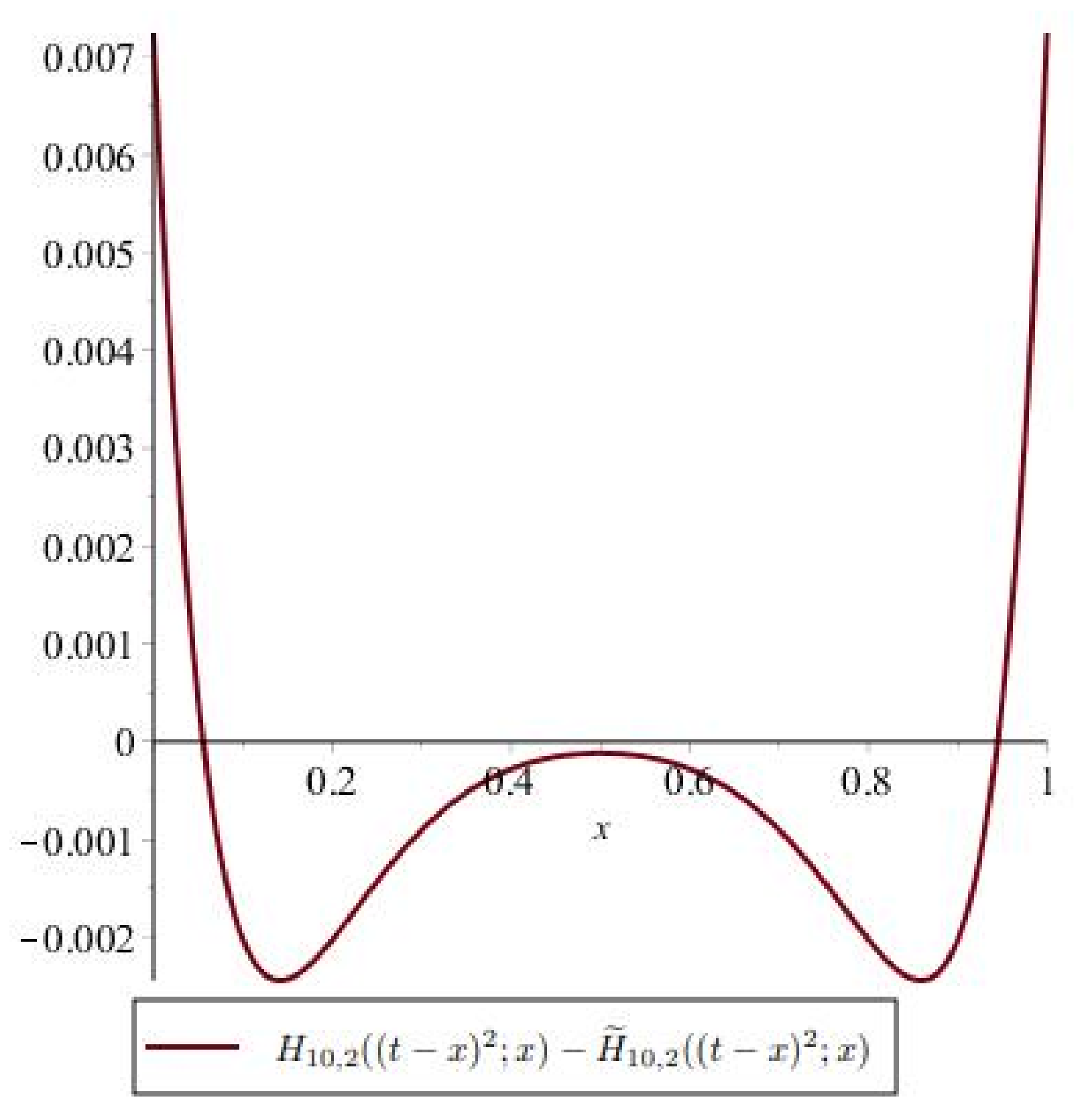
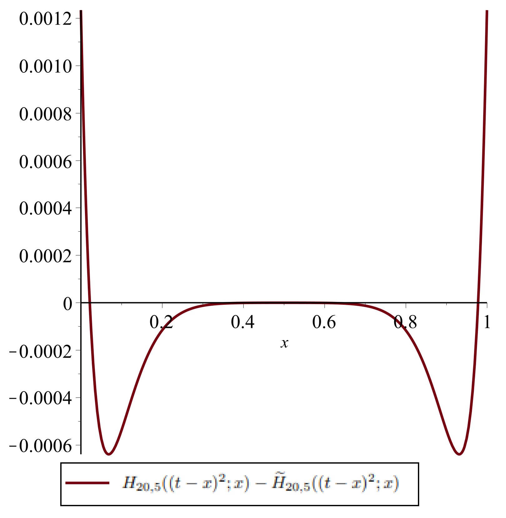
5. Differences in Positive Linear Operators

This section deals with estimates of the differences between classical operators and modified operators. Very recently, estimates of the differences of certain positive linear operators were obtained in [14,15,16,17,18].

Let $E\left(I\right)$ be a space of real-valued continuous functions on an interval $I\subset \mathbb{R}$ containing the polynomials. Denote $e_i\left(x\right):=x^i,x\in I$, $i\in \mathbb{N}$ and

$${\displaystyle {\mu }_i^F:=\frac{1}{i!}F{(e_1-b^F{e}_0)}^i,i\in \mathbb{N},}$$

where $F:E\left(I\right)\to \mathbb{R}$ is a positive linear functional, $F\left(e_0\right)=1$ and $b^F:=F\left(e_1\right)$.

Let $\mathcal{I}\subset \mathbb{N}$ and $A_k:E\left(I\right)\to \mathbb{R}$ and $B_k:E\left(I\right)\to \mathbb{R}$ be positive linear functionals such that $A_k\left(e_0\right)=B_k\left(e_0\right)=1$, $k\in \mathcal{I}$. Consider $p_k\in C\left(I\right)$ such that ${\displaystyle \sum _{k\in K}{p}_k=e_0}$ and $p_k\ge 0$, $k\in \mathcal{I}$.

Denote

$$D\left(I\right)=\left\{{\displaystyle f\in E\left(I\right)\left|{\displaystyle \sum _{k\in K}{A}_k\left(f\right)p_k\in C\left(I\right)}\right.\mathrm{and}\sum _{k\in K}{B}_k\left(f\right)p_k\in C\left(I\right)}\right\}.$$

Consider the positive linear operators $P:D\left(I\right)\to C\left(I\right)$ and $Q:D\left(I\right)\to C\left(I\right)$ defined, for $f\in D\left(I\right)$ as follows

$${\displaystyle P(f;x):=\sum _{k\in \mathcal{I}}{A}_k\left(f\right)p_k\left(x\right)\mathrm{and}Q(f;x):=\sum _{k\in \mathcal{I}}{B}_k\left(f\right)p_k\left(x\right).}$$

Denote ${\displaystyle \sigma \left(x\right):=\sum _{k\in \mathcal{I}}\left({\mu }_2^{A_k}+{\mu }_2^{B_k}\right)p_k\left(x\right)}$ and ${\displaystyle \delta :=\underset{k\in K}{sup}\left|b^{A_k}-b^{B_k}\right|}$.

Let ${\omega }_s(f,·)$, $s=1,2\dots$, be the usual moduli of smoothness of a function $f\in C\left(I\right)$.

Theorem 3.

[6] Let $f\in D\left(I\right)$ with $f^{\prime \prime }\in E_b\left(I\right)$. Then,

$$\left|(P-Q)(f;x)\right|\le \parallel f^{\prime \prime }\parallel \sigma \left(x\right)+{\omega }_1(f,\delta ),$$

(27)

where $E_b\left(I\right)$ is the space of all bounded functions $f\in E\left(I\right)$ endowed with supremum norm.

Theorem 4.

[6] Let $I=[0,1]$, $f\in C[0,1]$, ${\displaystyle 0<h\le \frac{1}{2},x\in [0,1]}$. Then,

$${\displaystyle \left|(P-Q)(f;x)\right|\le \frac{3}{2}\left(1+\frac{\sigma \left(x\right)}{h^2}\right){\omega }_2(f,h)+\frac{5\delta }{h}{\omega }_1(f,h).}$$

(28)

Using the above theorems and certain calculations from [6], some estimates of the differences between classical operators and modified operators are given in the next two propositions.

Proposition 2.

For Bernstein operators and modified Bernstein–Durrmeyer operators, the following properties hold:

(i)

$\left|\left(B_n-{\tilde{D}}_n\right)(f;x)\right|\le \sigma \left(x\right)\parallel f^{\prime \prime }\parallel +{\omega }_1\left(f;{\displaystyle \frac{n-2}{n(n+2)}}\right),f\in C^2[0,1],$

(ii)

${\displaystyle \left|\left(B_n-{\tilde{D}}_n\right)(f;x)\right|\le 3{\omega }_2(f,\sqrt{\sigma \left(x\right)})+\frac{5(n-2)}{n(n+2)\sqrt{\sigma \left(x\right)}}{\omega }_1\left(f,\sqrt{\sigma \left(x\right)}\right)}$, $f\in C[0,1],$

where$\sigma \left(x\right)={\displaystyle \frac{1}{2(n+3){(n+2)}^2}}\left\{x(1-x)n(n-1)+n+1\right\}-{\displaystyle \frac{n+1}{2{(n+2)}^2(n+3)}}\left\{{(1-x)}^n+x^n\right\}$.

Proposition 3.

The difference between Bernstein operators and modified Kantorovich operators verifies the following inequalities:

(i)

$\left|\left(B_n-{\tilde{K}}_n\right)(f;x)\right|\le \sigma \left(x\right)\parallel f^{\prime \prime }\parallel +{\omega }_1\left(f;{\displaystyle \frac{n-2}{2n(n+1)}}\right),f\in C^2[0,1],$

(ii)

${\displaystyle \left|\left(B_n-{\tilde{K}}_n\right)(f;x)\right|\le 3{\omega }_2(f,\sqrt{\sigma \left(x\right)})+\frac{5(n-2)}{2n(n+1)\sqrt{\sigma \left(x\right)}}{\omega }_1\left(f,\sqrt{\sigma \left(x\right)}\right)}$, $f\in C[0,1],$

where $\sigma \left(x\right)={\displaystyle \frac{1}{24{(n+1)}^2}}\left\{1-{(1-x)}^n-x^n\right\}$.

Proposition 4.

For Kantorovich operators and modified Kantorovich operators, the following property holds:

$$\left|\left(K_n-{\tilde{K}}_n\right)(f;x)\right|\le {\displaystyle \frac{1}{2(n+1)}}\parallel f^{\prime }\parallel \left\{{(1-x)}^n+x^n\right\},f\in C[0,1].$$

Proof. 

Using

$$\begin{array}{cc}\hfill {\displaystyle (n+1){\int }_0^{\frac{1}{n+1}}\left|f\left(t\right)-f\left(0\right)\right|dt}& \le (n+1)\parallel f^{\prime }\parallel {\int }_0^{\frac{1}{n+1}}tdt\hfill \\ \hfill & ={\displaystyle \frac{1}{2(n+1)}}\parallel f^{\prime }\parallel ,\hfill \end{array}$$

we obtain

$$\begin{array}{cc}\hfill & \left|\left(K_n-{\tilde{K}}_n\right)(f;x)\right|\hfill \\ \hfill & =\left|{\displaystyle (n+1){(1-x)}^n{\int }_0^{\frac{1}{n+1}}f\left(t\right)dt+(n+1)x^n{\int }_{\frac{n}{n+1}}^{1}f\left(t\right)dt-f\left(0\right){(1-x)}^n-f\left(1\right)x^n}\right|\hfill \\ \hfill & \le {\displaystyle \frac{1}{2(n+1)}}\parallel f^{\prime }\parallel \left\{{(1-x)}^n+x^n\right\}.\hfill \end{array}$$

Proposition 5.

The difference between Bernstein–Durrmeyer operators and modified Bernstein-Durrmeyer operators verifies the following inequalities:

$$\left|\left(D_n-{\tilde{D}}_n\right)(f;x)\right|\le {\displaystyle \frac{1}{n+2}}\parallel f^{\prime }\parallel \left\{{(1-x)}^n+x^n\right\},f\in C[0,1].$$

Proof. 

Using

$$\begin{array}{cc}\hfill \left|(n+1){\int }_0^1{(1-t)}^{n}f\left(t\right)dt-f\left(0\right)\right|& =\left|{\displaystyle (n+1){\int }_0^1{(1-t)}^n\left[f\left(t\right)-f\left(0\right)\right]dt}\right|\hfill \\ \hfill & \le (n+1)\parallel f^{\prime }\parallel {\int }_0^{1}t{(1-t)}^{n}dt\hfill \\ \hfill & ={\displaystyle \frac{1}{n+2}}\parallel f^{\prime }\parallel ,\hfill \end{array}$$

we obtain

$$\begin{array}{cc}\hfill & \left|\left(D_n-{\tilde{D}}_n\right)(f;x)\right|\hfill \\ \hfill & =\left|{\displaystyle (n+1){(1-x)}^n{\int }_0^1{(1-t)}^{n}f\left(t\right)dt+(n+1)x^n{\int }_0^1{t}^{n}f\left(t\right)dt-f\left(0\right){(1-x)}^n-f\left(1\right)x^n}\right|\hfill \\ \hfill & \le {\displaystyle \frac{1}{n+2}}\parallel f^{\prime }\parallel \left\{{(1-x)}^n+x^n\right\}.\hfill \end{array}$$

6. Conclusions and Perspectives

The preservation of affine functions is an important property of positive linear operators in Approximation Theory. It implies the interpolation property at extreme points. Several classical operators are suitable in this sense, but other ones are not, and consequently, they were modified in order to obtain the preservation property. Our paper is devoted to simpler modifications that guarantee interpolation at extreme points without implying the preservation of affine functions. The modified operators provide a better approximation near the extreme points. This can be seen in terms of moments and Voronovskaya-type formulas. Despite the fact that the images of monomials are rather complicated, we are able to give useful results concerning the limit of iterates of the modified operators, as well as estimates for differences involving classical and modified operators. We present general results formulated for operators defined on $C\left(X\right)$, the space of all real-valued, continuous functions on a compact Hausdorff space X. The illustrating examples are mainly concerned with operators defined on $C[0,1]$. A forthcoming paper will be devoted to the case when X is a simplex in $R^d$ or even a more general compact convex set.

References

1. Acu, A.M.; Raşa, I. Iterates and invariant measures for Markov operators. 2021, submitted.
2. Acu, A.M.; Bascanbaz-Tunca, G.; Raşa, I. Differences of Positive Linear Operators on Simplices. J. Funct. Spaces 2021, 2021, 5531577. [Google Scholar]
3. Acu, A.M.; Raşa, I. Estimates for the differences of positive linear operators and their derivatives. Numer. Algorithms 2020, 85, 191–208. [Google Scholar] [CrossRef] [Green Version]
4. Acu, A.M.; Hodis, S.; Raşa, I. Estimates for the Differences of Certain Positive Linear Operators. Mathematics 2020, 8, 798. [Google Scholar] [CrossRef]
5. Acu, A.M.; Hodis, A.M.S.; Raşa, I. A survey on estimates for the differences of positive linear operators. Constr. Math. Anal. 2018, 1, 113–127. [Google Scholar] [CrossRef]
6. Acu, A.M.; Raşa, I. New estimates for the differences of positive linear operators. Numer. Algorithms 2016, 73, 775–789. [Google Scholar] [CrossRef]
7. Brémaud, P. Markov Chains; Springer: New York, NY, USA, 1999. [Google Scholar]
8. Chung, K.L. Elementary Probability Theory with Stochastic Processes; Springer: Berlin, Germany, 1974. [Google Scholar]
9. Kemeny, J.G.; Snell, J.L. Finite Markov Chains; Springer: Berlin, Germany, 1976. [Google Scholar]
10. Păltănea, R. A class of Durrmeyer type operators preserving linear functions. Ann. Tiberiu Popoviciu Sem. Funct. Eq. Approx. Conv. (Cluj-Napoca) 2007, 5, 109–117. [Google Scholar]
11. Heilmann, M.; Raşa, I. A Nice Representation for a Link between Bernstein-Durrmeyer and Kantorovich Operators. In Proceedings of the Mathematics and Computing, ICMC 2017, Communications in Computer and Information Science, Haldia, India, 17–21 January 2017; Giri, D., Mohapatra, R., Begehr, H., Obaidat, M., Eds.; Springer: Singapore, 2017; Volume 655. [Google Scholar]
12. Heilmann, M.; Raşa, I. k-th order Kantorovich type modification of the operators Unρ. J. Appl. Funct. Anal. 2014, 9, 320–334. [Google Scholar]
13. Dancs, M. Differences of classical and modified operators. Gen. Math. 2021, 29, 3–12. [Google Scholar]
14. Gupta, V.; López-Pellicer, M.; Srivastava, H.M. Convergence estimates of a family of approximation operators of exponential type. Filomat 2020, 34, 4329–4341. [Google Scholar] [CrossRef]
15. Gupta, V.; Acu, A.M.; Srivastava, H.M. Difference of some positive linear approximation operators for higher-order derivatives. Symmetry 2020, 12, 915. [Google Scholar] [CrossRef]
16. Braha, N.L.; Mansour, T.; Srivastava, H.M. A parametric generalization of the Baskakov-Schurer-Szász-Stancu approximation operators. Symmetry 2021, 13, 980. [Google Scholar] [CrossRef]
17. Gupta, V.; Srivastava, H.M. A general family of the Srivastava-Gupta operators preserving linear functions. Eur. J. Pure Appl. Math. 2018, 11, 575–579. [Google Scholar] [CrossRef]
18. Usta, F. On approximation properties of a new construction of Baskakov operators. Adv. Differ. Equ. 2021, 2021, 269. [Google Scholar] [CrossRef]
Figure 1. Difference in the central moments for n = 10 , ρ = 2 .
Mathematics 09 02051 g001
Figure 2. Difference in the central moments for n = 20 , ρ = 5 .
Mathematics 09 02051 g002
Publisher’s Note: MDPI stays neutral with regard to jurisdictional claims in published maps and institutional affiliations.