Application of Decomposable Semi-Regenerative Processes to the Study of k-out-of-n Systems

Abstract

This paper aimed to demonstrate the capabilities of decomposable semi-regenerative processes for the investigation of the k-out-of-n system. Proposed in 1955 by W. Smith, the regeneration idea has come a long way in terms of development and has found widespread applications. First, we briefly recall the history of the development of the regeneration idea and the main results of the theory of regenerative, semi-regenerative, and decomposable semi-regenerative processes. Then, the methods of the theory of decomposable semi-regenerative processes are used for the study of a k-out-of-n renewable system with exponentially distributed life and generally distributed repair times of its components. This system is very important for practice and its special cases have previously been considered (including by the authors); however, only special cases and using other methods are considered herein. In the current paper, two scenarios of system repair after its failure are considered for the first time: the partial and the full system repair scenarios. For both scenarios, the time-dependent system state probabilities are calculated in terms of their Laplace transforms. The closed form representation of the stationary probabilities for both scenarios are also presented. These latest results represent a new contribution to the study of this system.

1. Introduction and Motivation

The paper aimed to demonstrate the capabilities of decomposable semi-regenerative processes for the investigation of k-out-of-n systems. In this paper, we use traditional symbols $\mathbb{P}$ and $\mathbb{E}$ to denote probability and expectation, respectively.

As a generalization of classical independence, the regeneration idea was proposed by W. Smith in 1955 [1]. For a stochastic process $X=\{X(t):t\in R\}$ with its flow of $\sigma$-algebras ${\mathcal{F}}_t^X$, it is supposed that a sequence of points of time — regeneration times $\{S_n:n=1,2,\cdots \}$—exists in which the process forgets its past, i.e., for any $\mathrm{\Gamma }$, it holds that:

$$\begin{array}{c}\hfill \mathbb{P}\{X(S_n+t)\in \mathrm{\Gamma }|{\mathcal{F}}_{S_n}^X\}=\mathbb{P}\{X(S_n+t)\in \mathrm{\Gamma }|S_n\}=\mathbb{P}\{X(S_1+t)\in \mathrm{\Gamma }\}.\end{array}$$

Here, the process X is known as a regenerative process (RP), and the intervals $[S_{n-1},S_n)$ and their lengths $T_n=S_n-S_{n-1}$ are called regeneration periods.

The state probabilities $\pi (t;\mathrm{\Gamma })$ of any RP can be calculated in terms of its state probabilities during a separate regeneration period${\pi }^{(1)}(t,\mathrm{\Gamma })=\mathbb{P}\{X(S_n+t)\in \mathrm{\Gamma },t<T_n\}$ in the form:

$$\begin{array}{ccc}\hfill \pi (t;\mathrm{\Gamma })& \equiv & \mathbb{P}\{X(t)\in \mathrm{\Gamma }\}=\underset{0}{\overset{t}{\int }}\mathbb{P}\{X(t-u)\in \mathrm{\Gamma },t-u<T\}H(du)\equiv \hfill \\ & \equiv & \underset{0}{\overset{t}{\int }}{\pi }^{(1)}(t-u,\mathrm{\Gamma })H(du),\hfill \end{array}$$

(1)

where $F(t)=\mathbb{P}\{T_n\le t\}$ and the renewal function of the process:

$$H(t)=\mathbb{E}\left[\sum _{n\ge 0}{1}_{\{S_n\le t\}}\right]=\sum _{n\ge 0}\mathbb{P}\{S_n\le t\}=\sum _{n\ge 0}{F}^{\star n}(t)$$

satisfies the equation below, where the symbol ”⋆” means convolution:

$$H(t)=F(t)+F\star H(t)\equiv F(t)+\underset{0}{\overset{t}{\int }}F(du)H(t-u).$$

(2)

Moreover, this approach also allows to prove the existence of stationary probabilities and gives its closed form representation in terms of the process distribution in a separate regeneration period:

$$\pi (\mathrm{\Gamma })=\underset{t\to \infty }{lim}\pi (t;\mathrm{\Gamma })=\frac{1}{\mathbb{E}[T_n]}\underset{0}{\overset{\infty }{\int }}{\pi }^{(1)}(t,\mathrm{\Gamma })dt.$$

(3)

However, if the process behavior in a separate regeneration period is complex enough and the probability distributions in it cannot be analytically represented, the more detailed investigation of the process can be performed by using Markov-type dependency, which leads to the construction of the theory of semi-Markov processes, (see E. Cinlar (1969) [2], J. Jacod (1971) [3], V. Korolyuk and A. Turbin (1976) [4], among others). The combination of these notions led to the introduction of semi-regenerative processes, which first appeared under different names such as semi-Markov processes with additional trajectories in 1966 (Klimov [5]), regeneration processes with several types of regeneration points in 1971 (Rykov and Yastrebenetsky [6]), before they were named semi-regenerative processes (SRP) thanks to E. Nummeline [7].

The difference between SRP and RP is the assumption that in its semi-regeneration points of time $S_n$, the future of the process does not depend on its past but depends on its present—the state of the process at the last semi-regeneration point of time $X(S_n)$. We will refer to them as regeneration states, and denote their set by E:

$$\begin{array}{c}\hfill \mathbb{P}\{X(S_n+t)\in \mathrm{\Gamma }|{\mathcal{F}}_{S_n}^X\}=\mathbb{P}\{X(S_n+t)\in \mathrm{\Gamma }|X(S_n)\}=\mathbb{P}\{X(S_1+t)\in \mathrm{\Gamma }|X(S_1)\}.\end{array}$$

The main characteristic of the SRP ([4,7,8]) is its semi-Markov matrix (SMM) $Q(t)={[Q_{ij}(t)]}_{ij\in E}$ with the components:

$$Q_{ij}(t)=\mathbb{P}\{X(S_{n+1})=j,T_n<t,|X(S_n)=i\}.$$

For semi-regenerative processes with a denumerable set of regeneration states E that start from regeneration states with an initial distribution $\alpha =\{{\alpha }_i,i\in E\}$, Formula (1) takes the following form:

$$\begin{array}{ccc}\hfill \pi (t,\mathrm{\Gamma })& \equiv & \mathbb{P}\{X(t)\in \mathrm{\Gamma }\}=\sum _{i\in E}{\alpha }_i\left[{\delta }_{ij}{\pi }_j^{(1)}(t,\mathrm{\Gamma })+\underset{0}{\overset{t}{\int }}{H}_{ij}(du){\pi }_j^{(1)}(t-u,\mathrm{\Gamma })\right],\hfill \end{array}$$

(4)

where ${\pi }_j^{(1)}(t,\mathrm{\Gamma })=\mathbb{P}\{X(S_n+t)\in \mathrm{\Gamma },t<T_n|X(S_n+0)=j\}$ is the process state probability distribution at SRP of type j, and $H(t)=[H_{ij}(t)]$ is its Markov renewal matrix (MRM) with:

$$H_{ij}(t)=\mathbb{E}\left[\sum _{n\ge 1}{1}_{\{S_n\le t,X(S_n)=j\}}|X(0)=i\right]={\left[\sum _{n\ge 1}{Q}^{*n}(t)\right]}_{ij\in E},$$

which satisfies to the following equation:

$$H(t)=Q(t)+Q\star H(t).$$

(5)

On the other hand, Formula (3) now takes the following form:

$$\pi (\mathrm{\Gamma })=\underset{t\to \infty }{lim}\pi (t,\mathrm{\Gamma })=\frac{1}{m}\underset{0}{\overset{\infty }{\int }}\sum _{j\in E}{\overline{\alpha }}_j{\pi }_j^{(1)}(t,\mathrm{\Gamma })dt,$$

(6)

where $\overline{\alpha }=\{{\overline{\alpha }}_i,(i\in E)\}$ are invariant probabilities of an embedded Markov chain, and $m={\sum }_{i\in E}{\overline{\alpha }}_i{\mathbb{E}}_i[T_n]$ is an expectation of the stationary regeneration period.

The next step in the generalization of the regeneration idea consists of finding, within the main regeneration period, some new regeneration time points and the construction of the so-called decomposable semi-regenerative process (DSRP). If the process behavior in some separate regeneration period $T_n$ is complex enough and its distribution cannot be analytically represented, sometimes it is possible to find within this period some embedded regeneration points of time $S_k^{(1)}(k=1,2,\cdots )$, in which the process forgets its past up to the present state $X^{(1)}\left(S_k^{(1)}\right)$ conditionally to its behavior in the embedded regeneration period $T_k^{(1)}=S_k^{(1)}-S_{k-1}^{(1)}$. The subset of embedded regeneration states of the process will be denoted by $E^{(1)}$. Since these are extended to any regeneration periods $T_n$, this procedure leads to the construction of DSRP. The strong definitions and details can be found in V. Rykov (1975) [9] (as can also be seen in [8,10]).

While analyzing the DSRP, the role of the ordinary MRM plays the appropriate embedded Markov renewal matrix (EMRM) $H^{(1)}(t)=[H_{ij}^{(1)}(t)]$ with components:

$$\begin{array}{c}{H}_{ij}^{(1)}(t)={\mathbb{E}}_i\left[\sum _{k\ge 0}{1}_{\{[0,t),j\}}\left(S_k^{(1)},X_k^{(1)}\right)1_{\{S_k^{(1)}<T_n\}}\right].\end{array}$$

This matrix study depends on the type of construction of the embedded regeneration points. There are different scenarios for building the embedded regeneration points’ construction. If they arise as $min[S_k^{(1)},T_n]$, then unlike Equations (2) and (5), for EMRM the following equation holds:

$$\begin{array}{ccc}\hfill & & H^{(1)}(t)=Q_1^{(1)}(t)+H^{(1)}\star Q^{(1)}(t)-Q(t),\hfill \end{array}$$

(7)

where the $Q(t)$ and $Q^{(1)}(t)$ are the SMM of the external and internal embedded periods and now the symbol ”⋆” means matrix-functional convolution.

However, in most practical situations, both internal and external regeneration times coincide with the time moments of entering the regeneration states. In this case, the external regeneration points are the moments when the process leaves the subset of the embedded regeneration states. In this case, the transition matrix for the embedded moments of regeneration $Q^{(1)}(t)={[Q_{ij}^{(1)}(t)]}_{ij\in E_1}$ is a sub-matrix of the main matrix $Q(t)$ with components from the subset of the embedded states $E^{(1)}$ and therefore it is a degenerate one. In this case, the equation for EMRM $H^{(1)}(t)={[H_{ij}^{(1)}(t)]}_{ij\in E_1}$ has the following form:

$$\begin{array}{c}\hfill H^{(1)}(t)=Q^{(1)}(t)+Q^{(1)}(t)\star H^{(1)}(t),\end{array}$$

and its solution is:

$$H^{(1)}(t)={(I-Q^{(1)}(t))}^{-1}{Q}^{(1)}(t)=\sum _{n\ge 1}\left[Q^{(1)*(n)}(t)\right],$$

and it is bounded for all t when $t\to \infty$ and tends to the mean number of visits of subset $E^{(1)}$.

Similarly to (4), if it is possible to find within a regeneration period of the first level $T_n^{(1)}$ embedded regeneration points of the second level $S_k^{(2)}$, then different characteristics within the regeneration period of the first level $T_n^{(1)}$ can be expressed in terms of its corresponding characteristics of the embedded RP of the second level regeneration period $T_k^{(2)}$. Particularly, for the one-dimensional distributions ${\pi }_i^{(1)}(t,\mathrm{\Gamma })$, the following representation holds:

$$\begin{array}{ccc}\hfill {\pi }_i^{(1)}(t,\mathrm{\Gamma })& \equiv & \mathbb{P}\left\{X^{(1)}\left(S_k^{(1)}+t\right)\in \mathrm{\Gamma }|X^{(1)}\left(S_k^{(1)}+0\right)=i\right\}=\hfill \\ \hfill & =& \sum _{j\in E}{\int }_0^t{H}_{ij}^{(1)}(du){\pi }_j^{(2)}(t-u,\mathrm{\Gamma })\equiv {\overrightarrow{H}}_i^{(1)}\star {\overrightarrow{\pi }}^{(2)}(t,\mathrm{\Gamma }),\hfill \end{array}$$

where:

$$\begin{array}{c}{\pi }_i^{(2)}(t,\mathrm{\Gamma })=\mathbb{P}\left\{X^{(1)}\left(S_k^{(1)}+t\right)\in \mathrm{\Gamma },t<T_{k+1}^{(2)}\mid X^{(1)}\left(S_k^{(1)}+0\right)=i\right\}\end{array}$$

is the process state probabilities during the embedded regeneration period of the second level and EMRM $H^{(1)}(t)$ satisfies Equation (7).

This procedure can be developed for the construction of DSRP with several levels of decomposition. The above system of embedded regeneration periods makes it possible to calculate the process distribution in terms of its distributions during the smallest regeneration periods, as can be seen for example in [8,11]. The limit theorem for SRPs allows calculating its stationary distributions.

In this paper, the methods of DSRP will be used for the investigation of a k-out-of-$n:F$ ($1\le k\le n$) system, which is defined as a repairable redundant system that consists of n components in parallel and fails when k of them fail. A k-out-of-$n:F$ configuration is a typical form of redundancy and systems of this type have been widely used in practical fields such as data transmission, networks, production management, transportation, voting systems, etc.

Due to the wide practical application area, a lot of papers are devoted to the study of k-out-of-n systems. The literature on such studies is vast (see for example Trivedi [12], Chakravarthy et al. [13] and the bibliography therein). The bibliography of later studies can be found in, e.g., in [14]. Most of these investigations deal with the systems under assumptions about components’ Poisson failure flow and exponential distribution of their repair time. In [15], M.S. Mustafa considered the k-out-of-n system with exponential life and the general repair time distribution of its components with the help of an embedded Markov chains method. Paper [16] contains a detailed analysis of 2-out-of-n and 3-out-of-n systems with exponential life and general repair time distributions.

In the series of our previous works, the bibliography of which one can find for example in [14], for an investigation of a renewable k-out-of-n system with the Poisson flow of its components’ failures and their arbitrarily distributed repair times, the so-called Markovization method was used. The method consists of the introduction of supplementary variables that allows describing the system behavior by a two-dimensional Markov process. This approach allows standing and proposing the way for the solution of one of the principal problems for system reliability investigation, namely: the problem of the sensitivity analysis of their output characteristics to the shape of input distributions. Some of the research results in this direction can be found, e.g., in [17,18] and in a series of our works, reference to which one can find, for example, in Chapter 9 of [19]. One may find recent reliability studies on k-out-of-n and related systems in [20,21]. Some applications for concrete problems in the oil and gas industry are also presented in [22,23].

In the current paper, to study the k-out-of-n system, we used an approach based on the methods of DSRP that allows extending the previous results and finding closed form representations for time-dependent and stationary characteristics of the system. In the future, these results can be used for the sensitivity analyses of the system characteristics to the shape of components’ repair time distributions.

The paper is organized as follows. In the next section, the problem setting and some notations will be introduced. In two next sections, the model with partial and full system repair will be studied. The paper ends with the conclusions and plans for further investigations.

2. State of Problem. Notations

Consider a repairable k-out-of-$n:F$ system, which can be considered as a repairable n-components system in parallel that fails when k of its components fail. For such a system, there exist at least two possible scenarios of system repair after its failure:

• Partial repair — when after the system’s failure, the repair of the component being repaired is prolonged, and after its end, the system passes to state $k-1$; or
• Full repair — when after the system’s failure, the repair of the whole system begins, and after its end, the system becomes as good as new, and enters state 0.

In this paper, we used the following assumptions:

• The lifetimes of the systems’ components are independent identically distributed (i.i.d.) random variables (r.v.’s) that are exponentially distributed with parameter $\alpha$.
• Failed components are repaired by a single facility and after repair become as good as new.
• Repair times are i.i.d. r.v.’s $B_i(i=1,2,\cdots )$ for partial and $G_i(i=1,2,\cdots )$ for full repair, respectively, with the common cumulative distribution functions (c.d.f.’s) $B(t)=\mathbb{P}\{B_i\le t\}$ and $G(t)=\mathbb{P}\{G_i\le t\}$.

Note that hereinafter, the random variables designated by letters without indices will imply the representatives of the corresponding sequences of i.i.d r.v.’s.

To study the system, we introduced the following notations:

• $\mathbb{P}\{·\},\mathbb{E}[·]$ — symbols of probability and expectation, symbols ${\mathbb{P}}_i\{·\},{\mathbb{E}}_i[·]$ are used for conditional probability and expectation, given that the initial state of the process is i;
• ${\mathsf{\Lambda }}_i$ is the random time to one of the system’s component failures, when it is in the state i;
• ${\lambda }_i=(n-i)\alpha$ is the parameter of this r.v. (intensity of the failure of one of the components—when the system is in the state i, sometimes the notation $(n-i)\alpha$ for this value is also used);
• $E=\{0,1,\cdots k\}$ is the system set of states, where j means the number of failed components and k is the system failure state;
• with this set of states, we define the random process $X=\{X(t),t\ge 0\}$ by the correlation:

  $$X(t)=j,\mathrm{if}\mathrm{in}\mathrm{time}\mathrm{epoch}t\mathrm{the}\mathrm{system}\mathrm{is}\mathrm{in}\mathrm{the}\mathrm{state}j\in E;$$
• system (and the process) state probabilities ${\pi }_j(t)=\mathbb{P}\{X(t)=j\};$
• T is the time to the system failure, $T=inf\{t:X(t)=k\}.$

Suppose also that initially, all system components are in good (UP) state, which means that the initial state of the process X is zero, $X(0)=0$. It is also supposed that immediate repairs of components and the whole system after its failure are impossible and both mean times to repair are finite:

$$B(0)=G(0)=0,\underset{0}{\overset{\infty }{\int }}(1-B(t))dt<\infty ,\underset{0}{\overset{\infty }{\int }}(1-G(t))dt<\infty .$$

Furthermore, in the paper, the system time-dependent state probabilities (t.d.s.p.’s):

$${\pi }_j(t)=\mathbb{P}\{X(t)=j\},$$

reliability function:

$$R(t)=\mathbb{P}\{T>t\},$$

and the steady state probabilities (s.s.p.’s):

$${\pi }_j=\underset{t\to \infty }{lim}{\pi }_j(t)$$

are calculated.

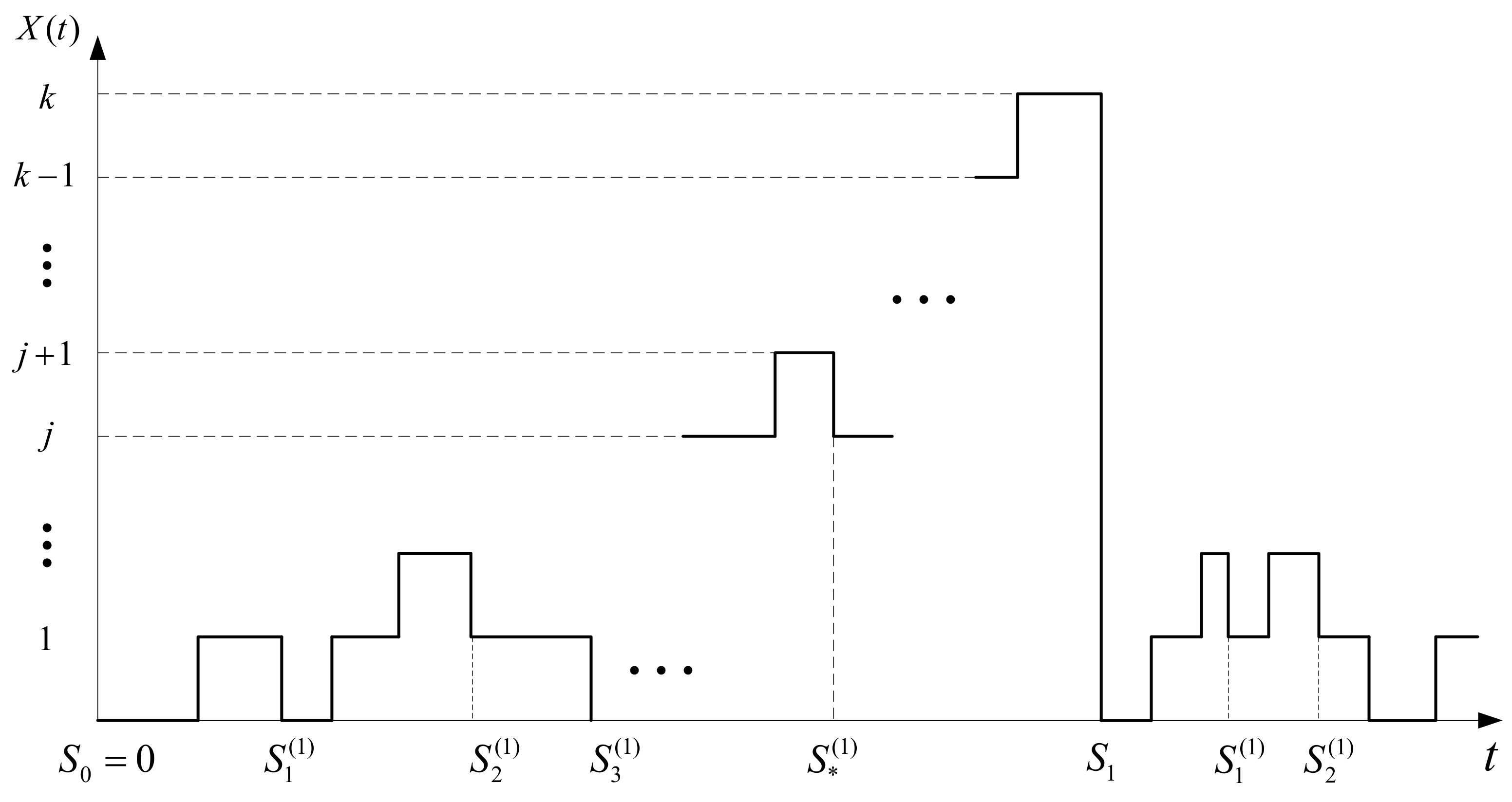
3. Partial Repair Regime

Considering first a partial repair regime, when after the system failure (when the system enters state k), the repair of the component being repaired continues and after its end, the system goes to state $k-1$.

3.1. Semi-Regenerative Process

In this case, we consider the process X as a semi-regenerative one (see Figure 1). Its regeneration time points $S_n$ of the type j are the repair completion times when the system enters state $j,X(S_n+0)=j$, semi-regeneration periods are $T_n=S_n-S_{n-1}$ and the regeneration set of states is $E_1=\{j:(j=\overline{0,k-1})\}$.

Recall first that the time-dependent state probabilities of the process X depend on the initial process distribution vector-row ${\overrightarrow{\alpha }}^{(0)}=\{{\alpha }_i^{(0)}:i\in E\}$. Thus, denoting by $\overrightarrow{\pi }(t)=\{{\pi }_j(t):j\in E\}$ the vector-row of the process state probabilities, and by $\mathrm{\Pi }(t)={[{\pi }_{ij}(t)]}_{ij\in E}$ the probability transition matrix of the process X, where:

$${\pi }_{ij}(t)=\mathbb{P}\{X(t)=j|X(0)=i\}\equiv {\mathbb{P}}_i\{X(t)=j\},(i,j\in E)$$

in matrix form, it holds that:

$$\overrightarrow{\pi }(t)={\overrightarrow{\alpha }}^{(0)}\mathrm{\Pi }(t).$$

On the other hand, according to the theory of semi-regenerative processes, as it was mentioned in the Introduction section, the process transition probabilities $\mathrm{\Pi }(t)={[{\pi }_{ij}(t)]}_{ij\in E}$ can be represented in the following form:

$$\mathrm{\Pi }(t)={\mathrm{\Pi }}^{(1)}(t)+H\star {\mathrm{\Pi }}^{(1)}(t)$$

(8)

in terms of corresponding state probabilities ${\mathrm{\Pi }}^{(1)}(t)={[{\pi }_{ij}^{(1)}(t)]}_{i\in E_1,j\in E}$ in separate regeneration periods, where:

$${\pi }_{ij}^{(1)}(t)=\mathbb{P}\{X(S_{n-1}+t)=j,t\le T_n|X(S_{n-1}+0)=i)\},(i\in E_1,j\in E)$$

and the Markov renewal matrix $H(t)={\left[H_{ij}(t)\right]}_{ij\in E_1}$ with:

$$H_{ij}(t)=\mathbb{E}\left[\sum _{n\ge 1}{1}_{\{S_n\le t,X(S_n)=j\}}|X(0)=i\right]\equiv {\mathbb{E}}_i\left[\sum _{n\ge 1}{1}_{\{S_n\le t,X(S_n)=j\}}\right].$$

Remark 1.

Note that the representation (8) is the solution of the equation:

$$\mathrm{\Pi }(t)={\mathrm{\Pi }}^{(1)}(t)+Q\star \mathrm{\Pi }(t).$$

It is known from the introduction that the MRM in matrix form satisfies the following equation:

$$H(t)=Q(t)+Q\star H(t),$$

(9)

where $Q(t)={[Q_{ij}(t)]}_{ij\in E_1}$ is the Semi-Markov matrix of the process X with:

$$Q_{ij}(t)=\mathbb{P}\{X(S_n+0)=j,T_n\le t|X(S_{n-1}+0)=i\}.$$

Equations (8) and (9) show that the best way to calculate the process time-dependent probabilities is using Laplace (LT) and Laplace–Stiltjes transforms (LST). Thus, further, along with all time-dependent characteristics of the process, we will present their LT or LST. Denote by

$$\tilde{\mathrm{\Pi }}(s)=\underset{0}{\overset{\infty }{\int }}{e}^{-st}\mathrm{\Pi }(t)dt,{\tilde{\mathrm{\Pi }}}^{(1)}(s)=\underset{0}{\overset{\infty }{\int }}{e}^{-st}{\mathrm{\Pi }}^{(1)}(t)dt,\mathrm{and}\tilde{h}(s)=\underset{0}{\overset{\infty }{\int }}{e}^{-st}H(dt)$$

LT of matrices $\mathrm{\Pi }(t),{\mathrm{\Pi }}^{(1)}(t)$ and LST of matrix $H(t)$. Following this approach, the transition to the LT in relation to (8) and LST in (9) gives:

$$\tilde{\mathrm{\Pi }}(s)=(I+\tilde{h}(s)){\tilde{\mathrm{\Pi }}}^{(1)}(s),\mathrm{and}\tilde{h}(s)=\tilde{q}(s)+\tilde{q}(s)\tilde{h}(s).$$

The solution of the last equation is $\tilde{h}(s)={(I-\tilde{q}(s))}^{-1}\tilde{q}(s).$

This leads to the following result:

$$\begin{array}{ccc}\hfill \tilde{\mathrm{\Pi }}(s)& =& (I+\tilde{h}(s)){\tilde{\mathrm{\Pi }}}^{(1)}(s)=[I+{(I-\tilde{q}(s))}^{-1}\tilde{q}(s)]{\tilde{\mathrm{\Pi }}}^{(1)}(s)=\hfill \\ & =& \left[I+\left(\sum _{n\ge 0}{\tilde{q}}^n(s)\right)\tilde{q}(s)\right]{\tilde{\mathrm{\Pi }}}^{(1)}(s)={(I-\tilde{q}(s))}^{-1}{\tilde{\mathrm{\Pi }}}^{(1)}(s).\hfill \end{array}$$

(10)

Thus, our goal was to calculate the matrix of the process state probabilities ${\mathrm{\Pi }}^{(1)}(t)$ in separate semi-regenerative periods and the SMM $Q(t)={[Q_{ij}(t)]}_{ij\in E_1}$ of the process X. In order to calculate the last matrix, we denote by $p_{ij}(t)$ the probability that the non-repairable k-out-of-$n:F$ system during time t passes from state i to state j, i.e., that during time t, $j-i$ components of the system out of $n-i$ that are working in the beginning of the interval fail. Denote by $P_{ik}(t)$ the probability that starting from state i, the system leaves the subset of working states during time t, i.e., the probability that during time t, at least $k-i$ system components fail out of $n-i$ that are working in the beginning of the time interval. These probabilities are obtained as follows:

$$p_{ij}(t)=\left(\genfrac{}{}{0pt}{}{n-i}{j-i}\right){(1-e^{-\alpha t})}^{j-i}{e}^{-(n-j)\alpha t},$$

and:

$$P_{ik}(t)=\sum _{j\ge k}{p}_{ij}(t)=1-\sum _{i\le j\le k-1}{p}_{ij}(t).$$

Note that the latter probability is the lifetime c.d.f. of a non-repairable k-out-of-n system.

To simplify further calculations, we represent these probabilities by Newton’s binomial formula as the sum and with the substitution ${\lambda }_i=(n-i)\alpha$ (note that the symbol $\alpha$ is also possible) we obtain:

$$p_{ij}(t)=\left(\genfrac{}{}{0pt}{}{n-i}{j-i}\right)\sum _{m=0}^{j-i}{(-1)}^m\left(\genfrac{}{}{0pt}{}{j-i}{m}\right)e^{-{\lambda }_{j-m}t}.$$

(11)

and:

$$P_{ik}(t)=\sum _{j\ge k}\left(\genfrac{}{}{0pt}{}{n-i}{j-i}\right)\sum _{m=0}^{j-i}{(-1)}^m\left(\genfrac{}{}{0pt}{}{j-i}{m}\right)e^{-{\lambda }_{j-m}t}.$$

(12)

Using these notations for the differentials of the SMM, the following lemma holds.

Lemma 1.

The differentials of the SMM of the process X are:

$$\begin{array}{ccc}\hfill Q_{0j}(dt)& =& \underset{0}{\overset{t}{\int }}{\lambda }_0{e}^{-{\lambda }_{0}u}du{p}_{1j+1}(t-u)B(dt-u),j=\overline{0,k-2};\hfill \\ \hfill Q_{0k-1}(dt)& =& \underset{0}{\overset{t}{\int }}{\lambda }_0{e}^{-{\lambda }_{0}u}du{P}_{1k}(t-u)B(dt-u);\hfill \\ \hfill Q_{ij}(dt)& =& p_{ij+1}(t)B(dt),(i=\overline{1,k-2},j=\overline{i-1,k-2});\hfill \\ \hfill Q_{ik-1}(dt)& =& P_{ik}(t)B(dt),\hfill \end{array}$$

(13)

and their LST ${\tilde{q}}_{ij}(s)={\int }_0^{\infty }{e}^{-st}{Q}_{ij}(dt)$ equals:

$$\begin{array}{ccc}\hfill {\tilde{q}}_{0j}(s)& =& {\displaystyle \frac{{\lambda }_0}{s+{\lambda }_0}}\left(\genfrac{}{}{0pt}{}{n-1}{j}\right)\sum _{l=0}^j{(-1)}^{j-l}\left(\genfrac{}{}{0pt}{}{j}{l}\right)\tilde{b}(s+{\lambda }_{l+1}),j=\overline{0,k-2};\hfill \\ \hfill {\tilde{q}}_{0k-1}(s)& =& {\displaystyle \frac{{\lambda }_0}{s+{\lambda }_0}}\sum _{j\ge k}\left(\genfrac{}{}{0pt}{}{n-1}{j-1}\right)\sum _{l=1}^j{(-1)}^{j-l}\left(\genfrac{}{}{0pt}{}{j-1}{j-l}\right)\tilde{b}(s+{\lambda }_l);\hfill \\ \hfill {\tilde{q}}_{ij}(s)& =& \left(\genfrac{}{}{0pt}{}{n-i}{j-i+1}\right)\sum _{l=j}^{i-1}{(-1)}^{j-l}\left(\genfrac{}{}{0pt}{}{j-i+1}{j-l}\right)\tilde{b}(s+{\lambda }_{l+1});\hfill \\ \hfill {\tilde{q}}_{ik-1}(s)& =& \sum _{j\ge k}\left(\genfrac{}{}{0pt}{}{n-i}{j-i}\right)\sum _{l=j}^i{(-1)}^{j-l}\left(\genfrac{}{}{0pt}{}{j-i}{j-l}\right)\tilde{b}(s+{\lambda }_l).\hfill \end{array}$$

(14)

Proof. 

Indeed, in order for the system in some regeneration epoch to occur in state $j\le ,wherek-2$ is in the previous regeneration epoch in state 0, it is necessary and sufficient that at some time point u, before time point t, one of the system components fails with the probability ${\lambda }_0{e}^{-{\lambda }_{0}u}du$, then during the remaining time $t-u$, another j component fails with probability $p_{1j+1}(t-u)$ and the originally failed component is repaired in the small vicinity of the time point t with probability $B(dt-u)$.

In a similar way, in order for the system in some regeneration epoch to occur in state $k-1$ while being in the previous one—in state 0—it is necessary and sufficient that, at some time point u before t, one of the system components fails with probability ${\lambda }_0{e}^{-{\lambda }_{0}u}du$, then during the remaining time $t-u$, it must reach state k with probability $P_{1k}(t-u)$ and the originally failed component is repaired in the small vicinity of the time point t with probability $B(dt-u)$.

Analogously, in order for the system in some regeneration epoch to occur in state j while being in the previous one—in state i—it is necessary and sufficient that the repair of the component under repair ends with probability $B(dt)$, while other $j+1-i$ components fail during time t with probability $p_{ij+1}(t)$.

Finally, in order for the system in some regeneration epoch to occur in state $k-1$ while being in the previous one—in state i—it must reach state k with probability $P_{ik}(t)$ and return to state $k-1$ due to the end of repair of the component under repair with probability $B(dt)$.

The proof of expression (14) follows from passing to LST in Formula (13) with the help of expressions (11) and (12):

$$\begin{array}{ccc}\hfill {\tilde{q}}_{0j}(s)& =& {\int }_0^{\infty }{e}^{-st}{Q}_{0j}(dt)=\hfill \\ & =& {\lambda }_0{\int }_0^{\infty }{e}^{-st}{\int }_0^t{e}^{-{\lambda }_{0}u}{p}_{1j+1}(t-u)B(dt-u)du=\hfill \\ & =& {\displaystyle \frac{{\lambda }_0}{s+{\lambda }_0}}{\int }_0^{\infty }{e}^{-sv}{p}_{1j+1}(v)B(dv)=\hfill \\ & =& {\displaystyle \frac{{\lambda }_0}{s+{\lambda }_0}}\left(\genfrac{}{}{0pt}{}{n-1}{j}\right)\sum _{m=0}^j{(-1)}^m\left(\genfrac{}{}{0pt}{}{j}{m}\right)\tilde{b}(s+{\lambda }_{j+1-m});\hfill \end{array}$$

$$\begin{array}{ccc}\hfill {\tilde{q}}_{0k-1}(s)& =& {\int }_0^{\infty }{e}^{-st}{Q}_{0k-1}(dt)=\hfill \\ & =& {\lambda }_0{\int }_0^{\infty }{e}^{-st}{\int }_0^t{e}^{-{\lambda }_{0}u}{P}_{1k}(t-u)B(dt-u)du=\hfill \\ & =& {\displaystyle \frac{{\lambda }_0}{s+{\lambda }_0}}{\int }_0^{\infty }{e}^{-sv}{P}_{1k}(v)B(dv)=\hfill \\ & =& {\displaystyle \frac{{\lambda }_0}{s+{\lambda }_0}}\sum _{j\ge k}\left(\genfrac{}{}{0pt}{}{n-1}{j-1}\right)\sum _{m=0}^{j-1}{(-1)}^m\left(\genfrac{}{}{0pt}{}{j-1}{m}\right)\tilde{b}(s+{\lambda }_{j-m});\hfill \end{array}$$

$$\begin{array}{ccc}\hfill {\tilde{q}}_{ij}(s)& =& {\int }_0^{\infty }{e}^{-st}{Q}_{ij}(dt)={\int }_0^{\infty }{e}^{-st}{p}_{ij+1}(t)B(dt)=\hfill \\ & =& \left(\genfrac{}{}{0pt}{}{n-i}{j-i+1}\right)\sum _{m=0}^{j-i+1}{(-1)}^m\left(\genfrac{}{}{0pt}{}{j-i+1}{m}\right)\tilde{b}(s+{\lambda }_{j+1-m});\hfill \end{array}$$

$$\begin{array}{ccc}\hfill {\tilde{q}}_{ik-1}(s)& =& {\int }_0^{\infty }{e}^{-st}{Q}_{ik-1}(dt)={\int }_0^{\infty }{e}^{-st}{P}_{ik}(t)B(dt)=\hfill \\ & =& \sum _{j\ge k}\left(\genfrac{}{}{0pt}{}{n-i}{j-i}\right)\sum _{m=0}^{j-i}{(-1)}^m\left(\genfrac{}{}{0pt}{}{j-i}{m}\right)\tilde{b}(s+{\lambda }_{j-m}).\hfill \end{array}$$

By substitution $l=j-m$, we obtain Formula (14). □

In the next section, the behavior of the process X in a separate semi-regeneration period is considered.

3.2. Behavior of the Process in a Separate Semi-Regeneration Period

The system time-dependent state probabilities in separate regeneration periods are given in the following lemma.

Lemma 2.

The system time-dependent state probabilities in separate semi-regeneration periods are:

$$\begin{array}{ccc}\hfill {\pi }_{00}^{(1)}(t)& =& e^{-{\lambda }_{0}t};\hfill \\ \hfill {\pi }_{0j}^{(1)}(t)& =& \underset{0}{\overset{t}{\int }}{\lambda }_0{e}^{-{\lambda }_{0}u}{p}_{1j}(t-u)(1-B(t-u))du,(j=\overline{1,k-1});\hfill \\ \hfill {\pi }_{0k}^{(1)}(t)& =& \underset{0}{\overset{t}{\int }}{\lambda }_0{e}^{-{\lambda }_{0}u}{P}_{1k}(t-u)(1-B(t-u))du;\hfill \\ \hfill {\pi }_{ij}^{(1)}(t)& =& p_{ij}(t)(1-B(t)),(1\le i\le j\le k-1);\hfill \\ \hfill {\pi }_{ik}^{(1)}(t)& =& P_{ik}(t)(1-B(t)),(i=\overline{1,k-1}).\hfill \end{array}$$

(15)

The LT ${\tilde{\pi }}_{ij}^{(1)}(s)$ of the process state probabilities ${\pi }_{ij}^{(1)}(t)$ in the separate embedded regeneration period are:

$$\begin{array}{ccc}\hfill {\tilde{\pi }}_{00}^{(1)}(s)& =& {\displaystyle \frac{1}{s+{\lambda }_0}};\hfill \\ \hfill {\tilde{\pi }}_{0j}^{(1)}(s)& =& {\displaystyle \frac{{\lambda }_0}{s+{\lambda }_0}}\left(\genfrac{}{}{0pt}{}{n-1}{j-1}\right)\sum _{l=0}^j{(-1)}^{j-l}\left(\genfrac{}{}{0pt}{}{j-1}{l-1}\right){\displaystyle \frac{1-\tilde{b}(s+{\lambda }_l)}{s+{\lambda }_l}},(j=\overline{1,k-1});\hfill \\ \hfill {\tilde{\pi }}_{0k}^{(1)}(s)& =& {\displaystyle \frac{{\lambda }_0}{s+{\lambda }_0}}\sum _{j\ge k}\left(\genfrac{}{}{0pt}{}{n-1}{j-1}\right)\sum _{l=0}^j{(-1)}^{j-l}\left(\genfrac{}{}{0pt}{}{j-1}{l-1}\right){\displaystyle \frac{1-\tilde{b}(s+{\lambda }_l)}{s+{\lambda }_l}};\hfill \\ \hfill {\tilde{\pi }}_{ij}^{(1)}(s)& =& \left(\genfrac{}{}{0pt}{}{n-i}{j-i}\right)\sum _{l=i}^{j+1}{(-1)}^{j-l}\left(\genfrac{}{}{0pt}{}{j-i}{l-i}\right){\displaystyle \frac{1-\tilde{b}(s+{\lambda }_l)}{s+{\lambda }_l}},(1\le i\le j\le k-1);\hfill \\ \hfill {\tilde{\pi }}_{ik}^{(1)}(s)& =& \sum _{j\ge k}\left(\genfrac{}{}{0pt}{}{n-i}{j-i}\right)\sum _{l=i}^{j+1}{(-1)}^{j-l}\left(\genfrac{}{}{0pt}{}{j-i}{l-i}\right){\displaystyle \frac{1-\tilde{b}(s+{\lambda }_l)}{s+{\lambda }_l}}.\hfill \end{array}$$

(16)

Proof. 

In fact, the semi-regeneration periods of the zero-type are ${\mathsf{\Lambda }}_0+B$, and the semi-regeneration periods of all other types are equal to the repair times B. Thus, in order for the process to be in state 0, at time t, within a separate zero-type regeneration period, it should not leave this state before the first component’s failure during time t with probability $e^{-{\lambda }_{0}t}$:

$$\begin{array}{c}\hfill {\pi }_{00}^{(1)}(t)={\mathbb{P}}_0\{X(t)=0,t<{\mathsf{\Lambda }}_0+B\}={\mathbb{P}}_0\{t<{\mathsf{\Lambda }}_0\}=e^{-{\lambda }_{0}t}.\end{array}$$

Analogously, in order for the system to occur in state j within a separate semi-regeneration period of zero-type, it is necessary and sufficient that at some time u before time t, one of the system’s components fails with the probability ${\lambda }_0{e}^{-{\lambda }_{0}u}du$ and during the remaining time $t-u$, exactly $j-1$ new components of the system fail with the probability $p_{1j}(t-u)$ before the repair of the first one ends with probability $(1-B(t-u))$:

$$\begin{array}{c}\hfill {\pi }_{0j}^{(1)}(t)={\mathbb{P}}_0\{X(t)=j,t<{\mathsf{\Lambda }}_0+B\}=\underset{0}{\overset{t}{\int }}{\lambda }_0{e}^{-{\lambda }_{0}u}du{p}_{1j}(t-u)(1-B(t-u)).\end{array}$$

Similarly, in order for the process to occur in state k during a separate semi-regeneration period of zero-type, it is necessary and sufficient that at some time u before t, one of the system’s components fails with the probability ${\lambda }_0{e}^{-{\lambda }_{0}u}du$ and during the remaining time $t-u$, the process reaches state k with the probability $P_{1k}(t-u)$ before the repair of the first one ending with the probability $(1-B(t-u))$:

$$\begin{array}{c}\hfill {\pi }_{0k}^{(1)}(t)={\mathbb{P}}_0\{X(t)=j,t<{\mathsf{\Lambda }}_0+B\}=\underset{0}{\overset{t}{\int }}{\lambda }_0{e}^{-{\lambda }_{0}u}du{P}_{1k}(t-u)(1-B(t-u))\end{array}$$

Analogously, in order for the process to be in state j at time t in a separate i-th type semi-regeneration period, it is necessary and sufficient that during this time period, the repair does not end with probability $1-B(t)$, and that during this time period, the system passes from state i to state j with probability $p_{ij}(t)$ that is equal to:

$$\begin{array}{ccc}\hfill {\pi }_{ij}^{(1)}(t)& =& {\mathbb{P}}_i\{X(t)=j,t<B\}=p_{ij}(t)(1-B(t)).\hfill \end{array}$$

The same arguments lead to the end of Formula (15):

$$\begin{array}{ccc}\hfill {\pi }_{ik}^{(1)}(t)& =& P_{ik}(t)(1-B(t)).\hfill \end{array}$$

The proof of Formula (16) follows from passing to LT in expression (15) with the help of representations (11) and (12):

$$\begin{array}{ccc}\hfill {\tilde{\pi }}_{00}^{(1)}(s)& =& \underset{0}{\overset{t}{\int }}{e}^{-t(s+{\lambda }_0)}dt={\displaystyle \frac{1}{s+{\lambda }_0}};\hfill \end{array}$$

$$\begin{array}{ccc}\hfill {\tilde{\pi }}_{0j}^{(1)}(s)& =& \underset{0}{\overset{t}{\int }}{e}^{-st}\underset{0}{\overset{t}{\int }}{\lambda }_0{e}^{-{\lambda }_{0}u}du{p}_{1j}(t-u)(1-B(t-u))=\hfill \\ & =& {\displaystyle \frac{{\lambda }_0}{s+{\lambda }_0}}\underset{0}{\overset{\infty }{\int }}{e}^{-st}{p}_{1j}(t)(1-B(t))dt={\displaystyle \frac{{\lambda }_0}{s+{\lambda }_0}}{\tilde{\pi }}_{1j}^{(1)}(s)\hfill \\ & =& {\displaystyle \frac{{\lambda }_0}{s+{\lambda }_0}}\left(\genfrac{}{}{0pt}{}{n-1}{j-1}\right)\sum _{m=0}^{j-1}{(-1)}^m\left(\genfrac{}{}{0pt}{}{j-1}{m}\right){\displaystyle \frac{1-\tilde{b}(s+{\lambda }_{j-m})}{s+{\lambda }_{j-m}}};\hfill \end{array}$$

$$\begin{array}{ccc}\hfill {\tilde{\pi }}_{0k}^{(1)}(s)& =& \underset{0}{\overset{t}{\int }}{e}^{-st}\underset{0}{\overset{t}{\int }}{\lambda }_0{e}^{-{\lambda }_{0}u}du{P}_{1k}(t-u)(1-B(t-u))=\hfill \\ & =& {\displaystyle \frac{{\lambda }_0}{s+{\lambda }_0}}\underset{0}{\overset{\infty }{\int }}{e}^{-st}{P}_{1k}(t)(1-B(t))dt=\hfill \\ & =& {\displaystyle \frac{{\lambda }_0}{s+{\lambda }_0}}\left[{\displaystyle \frac{1-\tilde{b}(s)}{s}}-\sum _{1\le j\le k-1}\left(\genfrac{}{}{0pt}{}{n-1}{j-1}\right)\sum _{m=0}^{j-1}{(-1)}^m\left(\genfrac{}{}{0pt}{}{j-1}{m}\right){\displaystyle \frac{1-\tilde{b}(s+{\lambda }_{j-m})}{s+{\lambda }_{j-m}}}\right];\hfill \end{array}$$

$$\begin{array}{ccc}\hfill {\tilde{\pi }}_{ij}^{(1)}(s)& =& \underset{0}{\overset{\infty }{\int }}{e}^{-st}{p}_{ij}(t)(1-B(t))dt=\hfill \\ & =& \left(\genfrac{}{}{0pt}{}{n-i}{j-i}\right)\sum _{m=0}^{j-i}{(-1)}^m\left(\genfrac{}{}{0pt}{}{j-i}{m}\right){\displaystyle \frac{1-\tilde{b}(s+{\lambda }_{j-m})}{s+{\lambda }_{j-m}}};\hfill \end{array}$$

$$\begin{array}{ccc}\hfill {\tilde{\pi }}_{ik}^{(1)}(s)& =& \underset{0}{\overset{\infty }{\int }}{e}^{-st}{P}_{ik}(t)(1-B(t))dt=\hfill \\ & =& {\displaystyle \frac{1-\tilde{b}(s)}{s}}-\sum _{i\le j\le k-1}\left(\genfrac{}{}{0pt}{}{n-i}{j-i}\right)\sum _{m=0}^{j-i}{(-1)}^m\left(\genfrac{}{}{0pt}{}{j-i}{m}\right){\displaystyle \frac{1-\tilde{b}(s+{\lambda }_{j-m})}{s+{\lambda }_{j-m}}}.\hfill \end{array}$$

By substitution $l=j-m$, we obtain, Formula (16). □

3.3. Time-Dependent and Stationary Probabilities

By combining the results obtained above, the following theorem holds:

Theorem 1.

The LT of the time-dependent state probabilities of the process X in matrix form is given by equality (10):

$$\tilde{\mathrm{\Pi }}(s)={(I-\tilde{q}(s))}^{-1}{\tilde{\mathrm{\Pi }}}^{(1)}(s),$$

where components ${\tilde{\pi }}_{ij}^{(1)}(s)$ of the matrix ${\tilde{\mathrm{\Pi }}}^{(1)}(s)$ are given by Formula (16) from Lemma 2, and components ${\tilde{q}}_{lj}(s)$ of matrix $\tilde{q}(s)$ given by Formula (14) from Lemma 1.

The steady state probabilities of the process could be calculated by passing to the limit in the last equality. However, it would be preferable to use the limit theorem for the transition probabilities of semi-regenerative processes.

Theorem 2.

The stationary regime of the considered system under partial repair scenario exists and the steady state probabilities equal:

$${\pi }_j=\frac{1}{m}\sum _{0\le l\le j\wedge (k-1)}{\alpha }_l{\tilde{\pi }}_{lj}^{(1)}(0),(j=\overline{0,k}),$$

(17)

where $\overrightarrow{\alpha }=\{{\alpha }_l:l\in E_1\}$ satisfies the system of equations:

$${\overrightarrow{\alpha }}^{\prime }={\overrightarrow{\alpha }}^{\prime }\tilde{q}(0),\sum _{0\le l\le k-1}{\alpha }_l=1,$$

(18)

$m={\lambda }_0^{-1}({\alpha }_0+{\lambda }_{0}b)$, and ${\tilde{\pi }}_{ij}^{(1)}(0)$ can be found from Formula (16) of Lemma 2.

Proof. 

The embedded Markov chain of the process X is finite and irreducible. Thus, its invariant probabilities exist and according to the limit theorem for transition probabilities of semi-regenerative processes and according to the Introduction from Equation (6) independently of the initial state for any $j=\overline{0,k}$, it holds that:

$$\begin{array}{ccc}\hfill {\pi }_j& =& \underset{t\to \infty }{lim}{\pi }_{ij}(t)=\frac{1}{m}\sum _{0\le l\le j\wedge (k-1)}{\alpha }_l\underset{0}{\overset{\infty }{\int }}{\pi }_{lj}^{(1)}(t)dt=\frac{1}{m}\sum _{0\le l\le j\wedge (k-1)}{\alpha }_l{\tilde{\pi }}_{lj}^{(1)}(0),\hfill \end{array}$$

where vector $\overrightarrow{\alpha }=\{{\alpha }_l:l\in E_1\}$ is the invariant probability measure of the embedded Markov chain that satisfies the system of Equation (18) and m is the mean semi-regenerative period $m=\sum _{0\le l\le k-1}{\alpha }_l{\mathbb{E}}_l[T].$ Taking into account that the zero-type semi-regeneration period is equal to ${\mathsf{\Lambda }}_0+B$ and all others equal B, it is possible to show that:

$$m={\alpha }_0({\lambda }_0^{-1}+b)+(1-{\alpha }_0)b=\frac{1}{{\lambda }_0}({\alpha }_0+{\lambda }_{0}b).$$

 □

3.4. Example 1

As an example, we consider a special case of a 2-out-of-$n:F$ system. To find the s.s.p. of the system, it is necessary to calculate the LST of SMM $\tilde{Q}(s)$ as well as the LT of the process state probabilities in the SRP ${\tilde{\mathrm{\Pi }}}^{(1)}(s)$. From Lemma 1, we find $\tilde{Q}(s)$ using Formulas (11) and (12):

$$\begin{array}{c}\hfill \tilde{Q}(s)=\left[\begin{array}{cc}{\displaystyle \frac{{\lambda }_0\tilde{b}({\lambda }_1+s)}{{\lambda }_0+s}}& {\displaystyle \frac{{\lambda }_0(\tilde{b}(s)-\tilde{b}({\lambda }_1+s))}{{\lambda }_0+s}}\\ \tilde{b}({\lambda }_1+s)& \tilde{b}(s)-\tilde{b}({\lambda }_1+s).\end{array}\right]\end{array}$$

Lemma 2 gives the representation of ${\tilde{\mathrm{\Pi }}}^{(1)}(s)$:

$$\begin{array}{c}\hfill {\tilde{\mathrm{\Pi }}}^{(1)}(s)=\left[\begin{array}{ccc}{\displaystyle \frac{1}{s+{\lambda }_0}}& {\displaystyle \frac{{\lambda }_0(1-\tilde{b}({\lambda }_1+s))}{({\lambda }_0+s)({\lambda }_1+s)}}& {\displaystyle \frac{{\lambda }_0}{{\lambda }_0+s}}\left({\displaystyle \frac{1-\tilde{b}(s)}{s}}-{\displaystyle \frac{1-\tilde{b}({\lambda }_1+s)}{{\lambda }_1+s}}\right)\\ 0& {\displaystyle \frac{1-\tilde{b}({\lambda }_1+s)}{{\lambda }_1+s}}& {\displaystyle \frac{1-\tilde{b}(s))}{s}}-{\displaystyle \frac{1-\tilde{b}({\lambda }_1+s))}{{\lambda }_1+s}}\end{array}\right]\end{array}$$

To find the stationary regime of the considered system, the invariant probability measure of the embedded Markov chain ${\overrightarrow{\alpha }}^{\prime }$ and the mean semi-regenerative period m should be calculated. From Equation (18) and Theorem 2, we obtain:

$${\alpha }_0=\tilde{b}({\lambda }_1),{\alpha }_1=1-\tilde{b}({\lambda }_1),m=b+\frac{\tilde{b}({\lambda }_1)}{{\lambda }_0}.$$

Finally, by using (17), we obtain the s.s.p. of the 2-out-of-n system:

$${\pi }_0=\frac{\tilde{b}({\lambda }_1)}{\tilde{b}({\lambda }_1)+{\lambda }_{0}b},{\pi }_1=\frac{{\lambda }_0(1-\tilde{b}({\lambda }_1))}{{\lambda }_1(\tilde{b}({\lambda }_1)+{\lambda }_{0}b)},{\pi }_2=\frac{{\lambda }_0({\lambda }_{1}b-(1-\tilde{b}({\lambda }_1)))}{{\lambda }_1(\tilde{b}({\lambda }_1)+{\lambda }_{0}b)}.$$

In the case of exponentially distributed repair time with LST $\tilde{b}(\lambda )=\frac{1}{1+\lambda b}$, the steady-state probabilities coincide with those, obtained for the birth and death process:

$${\pi }_0=\frac{1}{1+{\lambda }_{0}b+{\lambda }_0{\lambda }_1{b}^2},{\pi }_1=\frac{{\lambda }_{0}b}{1+{\lambda }_{0}b+{\lambda }_0{\lambda }_1{b}^2},{\pi }_2=\frac{{\lambda }_0{\lambda }_1{b}^2}{1+{\lambda }_{0}b+{\lambda }_0{\lambda }_1{b}^2}.$$

Note that the analytical results for the special case of a 3-out-of-n system were also verified, but due to their cumbersomeness, we do not present them. These results also coincide with those obtained for the simple Markov model.

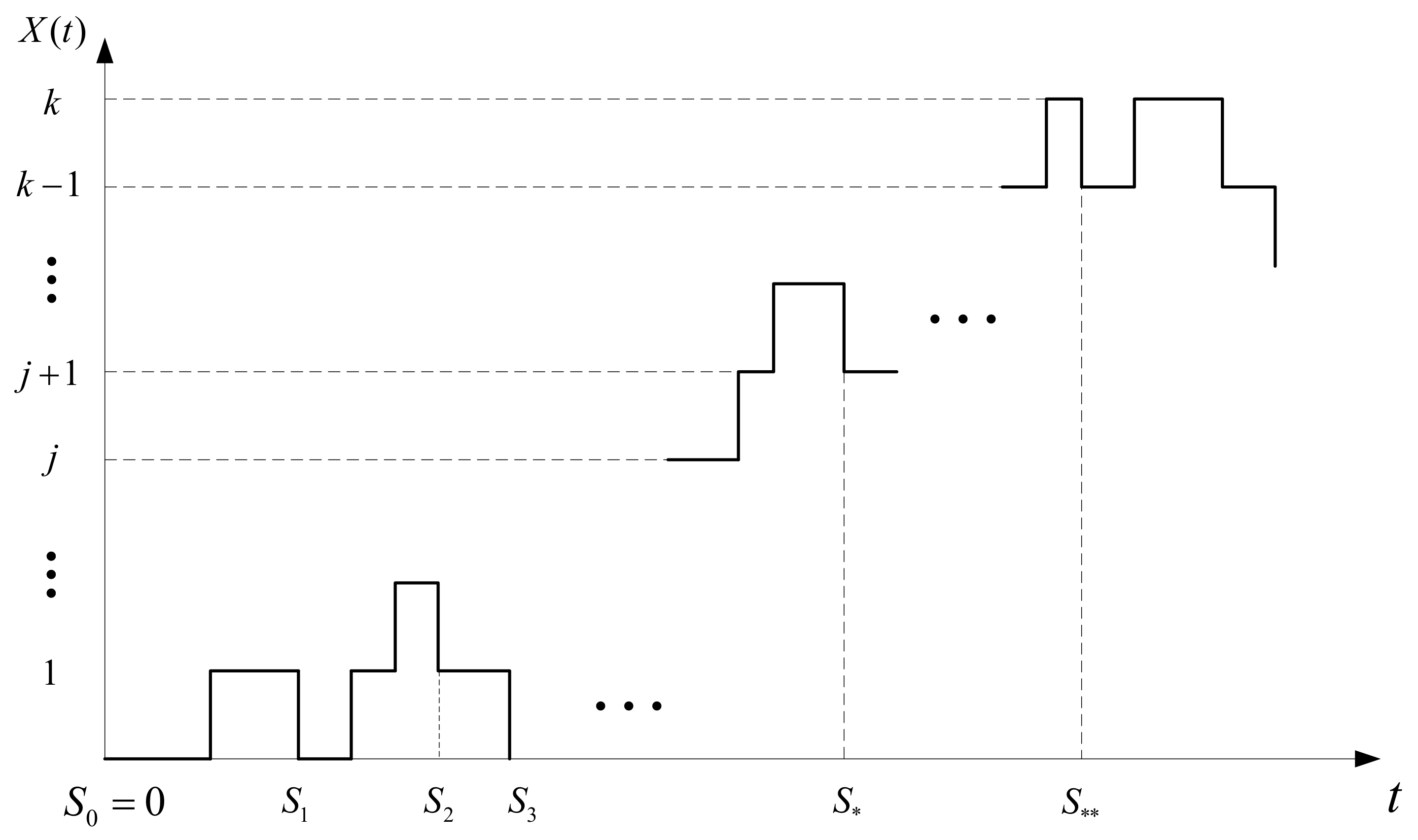
4. Full Repair Regime

To study the system’s behavior under the full repair regime, we consider the main process X as a regenerative one, whose regeneration points $S_n(n=1,2,\cdots ),S_0=0$ are the full repair completion times of the system after its failure. The regeneration periods ${\mathrm{\Theta }}_n=S_n-S_{n-1}$ of the process X consist of two terms: the system life times (times to system failure after repair) $F_n$ and the system repair times after failure $G_n:{\mathrm{\Theta }}_n=F_n+G_n$ (as can be seen in Figure 2). Denote by $F(t)=\mathbb{P}\{F_n\le t\}$ and $\mathrm{\Gamma }(t)=\mathbb{P}\{{\mathrm{\Theta }}_n\le t\}$ the common distribution function of r.v.’s $F_n$ and ${\mathrm{\Theta }}_n(n=1,2,\cdots )$, respectively.

4.1. The Main Regenerative Process

From the theory of regenerative processes in the sense of Smith, it follows that the time-dependent probabilities of the system can be represented in terms of the corresponding process state distribution ${\pi }_j^{(\mathrm{\Theta })}(t)=\mathbb{P}\{X(t)=j,t<\mathrm{\Theta }\}$ during a separate regeneration period $\mathrm{\Theta }$ as follows:

$${\pi }_j(t)={\pi }_j^{(\mathrm{\Theta })}(t)+\underset{0}{\overset{t}{\int }}{\pi }_j^{(\mathrm{\Theta })}(t-u)H(du).$$

(19)

Here, $H(t)$ is the corresponding renewal function which is generated by the c.d.f. $\mathrm{\Gamma }(t)=\mathbb{P}\{{\mathrm{\Theta }}_n\le t\}$ of r.v’s. ${\mathrm{\Theta }}_n$, and according to the Smith theorem, can be calculated as

$$H(t)=\sum _{n\ge 1}\mathbb{P}\{S_n\le t\}=\sum _{n\ge 1}{\mathrm{\Gamma }}^{(*n)}(t),$$

whose LST equals:

$$\tilde{h}(s)=\underset{0}{\overset{\infty }{\int }}{e}^{-st}H(dt)=\frac{\tilde{\gamma }(s)}{1-\tilde{\gamma }(s)},$$

(20)

where $\tilde{\gamma }(s)$ is LST of the c.d.f. $\mathrm{\Gamma }(t)$.

Thus, to study the process, we first need to calculate the distribution of the regeneration periods ${\mathrm{\Theta }}_n$, the corresponding renewal function $H(t)$ and the process distribution ${\pi }_j^{(\mathrm{\Theta })}(t)$ for them. Denote by $F_n(n=1,2,\cdots )$ time to the n-th system failure after its previous full repair, and by $F(t)$, their common distribution function $F(t)=\mathbb{P}\{F_n\le t\}$. We remind that the r.v. ${\mathrm{\Theta }}_n$ is the sum of two independent r.v.’s $F_n$ and $G_n$, as the distribution of the second one is supposed to be known and the distribution of the first one will be obtained, jointly with its LST later in Lemma 5 (see Remark 2 to it).

Now, we pass on to the calculation of the process state distribution ${\pi }_j^{(\mathrm{\Theta })}(t)$ in a separate regeneration period ${\mathrm{\Theta }}_n=F_n+G_n$. The process behavior in the separate regeneration period can be divided into two parts: the process behavior within a separate system lifetime $F_n$ and its behavior during the repair time $G_n$:

$$\{X(S_{n-1}+t)=j:t\le {\theta }_n\}=\left\{\begin{array}{cc}X(S_{n-1}+t)=j:\hfill & \mathrm{for}t\le F_n,j\ne k\hfill \\ k:\hfill & \mathrm{for}{F}_n<t\le {\mathrm{\Theta }}_n,j=k.\hfill \end{array}\right.$$

(21)

Thus, the process time-dependent state probabilities in a separate regeneration period are given in the following lemma.

Lemma 3.

The system state probabilities in a separate regeneration period Θ in terms of the corresponding probabilities within a separate system lifetime F are:

$${\pi }_j^{(\mathrm{\Theta })}(t)=(1-{\delta }_{jk}){\pi }_j^{(F)}(t)+{\delta }_{jk}\mathbb{P}\{F\le t<\mathrm{\Theta }\}$$

with their Laplace transform:

$${\tilde{\pi }}_j^{(\mathrm{\Theta })}(s)=(1-{\delta }_{jk}){\tilde{\pi }}_j^{(F)}(s)+{\delta }_{jk}\tilde{f}(s)\frac{1-\tilde{g}(s)}{s}.$$

(22)

Proof. 

The first equality of the lemma directly follows from the relation (21). In terms of LT, from this equality, it follows that:

$$\begin{array}{ccc}\hfill {\tilde{\pi }}_j^{(\mathrm{\Theta })}(s)& =& \underset{0}{\overset{\infty }{\int }}{e}^{-st}{\pi }_j^{(\mathrm{\Theta })}(t)dt=(1-{\delta }_{jk}){\tilde{\pi }}_j^{(F)}(s)+{\delta }_{jk}\underset{0}{\overset{\infty }{\int }}\mathbb{P}\{F\le t<\mathrm{\Theta }\}dt=\hfill \\ & =& (1-{\delta }_{jk}){\tilde{\pi }}_j^{(F)}(s)+{\delta }_{jk}\underset{0}{\overset{\infty }{\int }}{e}^{-st}dt\underset{0}{\overset{t}{\int }}(1-G(t-u))F(du)=\hfill \\ & =& (1-{\delta }_{jk}){\tilde{\pi }}_j^{(F)}(s)+{\delta }_{jk}\tilde{f}(s)\frac{1-\tilde{g}(s)}{s},\hfill \end{array}$$

which is the second equality of the lemma. □

The last equality shows that we need the process state distribution within a separate system lifetime F, which is considered in the following subsection.

4.2. Embedded Semi-Regenerative Process

Since the process behavior within the system lifetime F is rather complicated, the process X during this time will be considered as an embedded semi-regenerative process (ESRP) $X_n^{(1)}=\{X_n^{(1)}(t):t\ge 0\}$ with:

$$X_n^{(1)}(t)=X(S_{n-1}+t),t\le F_n.$$

Its semi-regeneration times $S_n^{(1)}$ of the type j are the same as for the semi-regenerative process in Section 3.1 (see Figure 2) except for the fact that now the process $X_n^{(1)}$ is considered in a separate main regeneration period and therefore never enters state $k-1$ after the system’s repair completion. Thus, there are only $k-1$ embedded regeneration states, $E^{(1)}=\{0,1,\cdots ,k-2\}.$

In order to study the behavior of the process before it enters state k, we denote by:

• $T_l^{(1)}=S_l^{(1)}-S_{l-1}^{(1)},l=1,2,\cdots$ the intervals between embedded semi-regeneration times of the ESRP $X^{(1)}$ (time points between the components repair completions);
• $Q^{(1)}(t)={[Q_{ij}^{(1)}(t)]}_{ij\in E^{(1)}}$ the embedded semi-Markov matrix (ESMM) whose components are the process transition probabilities between semi-regeneration times:

  $$Q_{ij}^{(1)}(t)=\mathbb{P}\{X^{(1)}(S_l^{(1)}+0)=j,T_l^{(1)}\le t|X^{(1)}(S_{l-1}^{(1)}+0)=i\};$$
• ${\overrightarrow{Q}}^{(1)}(t)=[Q_{ik}^{(1)}(t)]$ the vector-function, the components of which are the c.d.f.’s of the first passage time from state i to the absorbing state k by the ESRP along a monotone trajectory.
• $\overrightarrow{F}(t)=[F_{ik}(t)]$ the vector-function, the components of which are c.d.f.’s of the absorbing state k destination time by the ESRP starting from state $i(i=\overline{0,k-2})$;
• $H^{(1)}(t)={[H_{ij}^{(1)}(t)]}_{ij\in E^{(1)}}$ the embedded Markov renewal matrix, whose components are the conditional embedded renewal functions in the separate lifetime period:

  $$H_{ij}^{(1)}(t)=\mathbb{E}\left[\sum _{l\ge 1}{1}_{\{X^{(1)}(S_l^{(1)}+0)=j,S_l^{(1)}\le t\}}|X^{(1)}(S_0^{(1)})=i\right].$$

We start with the calculation of the ESMM $Q^{(1)}(t)={[Q_{ij}^{(1)}(t)]}_{ij\in E^{(1)}}$ of the ESRP $X^{(1)}$. To calculate it, we note that its components coincide with those from Section 3.1 that were determined in Lemma 1 except for the fact that now the process $X^{(1)}$ never enters state $k-1$ after the completion of the repair. Thus, they are only defined for $j\le k-2$, and in terms of Notations (11) and (12), are represented in differential form in Lemma 1. Thus, since the set of embedded regeneration states of the process $X^{(1)}$ is a proper subset of the set of states of the process X, its transition matrix is a degenerate matrix in contrast to the matrix of the previous section. Since the corresponding expressions are used later, we repeat them jointly with the components $Q_{ik}^{(1)}(t)$ of vector ${\overrightarrow{Q}}^{(1)}(t)$ of the probabilities of reaching the state k, together with their LST in the following lemma.

Lemma 4. 

(1) 

The differentials of the ESMM components of the process $X^{(1)}$ are:

$$\begin{array}{ccc}\hfill Q_{0j}^{(1)}(dt)& =& \underset{0}{\overset{t}{\int }}{\lambda }_0{e}^{-{\lambda }_{0}u}du{p}_{1j+1}(t-u)B(dt-u),(j=\overline{0,k-2}),\hfill \\ \hfill Q_{ij}^{(1)}(dt)& =& p_{ij+1}(t)B(dt),(i=\overline{1,k-2},j=\overline{i-1,k-2});\hfill \end{array}$$

(23)

while the differentials of the components of vector ${\overrightarrow{Q}}^{(1)}(dt)={[Q_{ik}^{(1)}(dt)]}_{i=\overline{0,k-2}}$ are:

$$\begin{array}{ccc}\hfill Q_{0k}^{(1)}(dt)& =& \underset{0}{\overset{t}{\int }}{\lambda }_0{e}^{-{\lambda }_{0}u}du{P}_{1k}(dt-u)(1-B(t-u)),\hfill \\ \hfill Q_{ik}^{(1)}(dt)& =& P_{ik}(dt)(1-B(t)).\hfill \end{array}$$

(2) 

The corresponding LST for the components of matrix $Q^{(1)}(t)$ are equal to:

$$\begin{array}{ccc}\hfill {\tilde{q}}_{0j}^{(1)}(s)& =& {\displaystyle \frac{{\lambda }_0}{s+{\lambda }_0}}\left(\genfrac{}{}{0pt}{}{n-1}{j}\right)\sum _{m=0}^j{(-1)}^m\left(\genfrac{}{}{0pt}{}{j}{m}\right)\tilde{b}(s+{\lambda }_{j+1-m}),(j=\overline{0,k-2});\hfill \\ \hfill {\tilde{q}}_{ij}^{(1)}(s)& =& \left(\genfrac{}{}{0pt}{}{n-i}{j-i+1}\right)\sum _{m=0}^{j-i+1}{(-1)}^m\left(\genfrac{}{}{0pt}{}{j-i+1}{m}\right)\tilde{b}(s+{\lambda }_{j+1-m}),\hfill \\ & & (i=\overline{1,k-2},j=\overline{i-1,k-2});\hfill \end{array}$$

(24)

while the corresponding LST for the components of vector ${\overrightarrow{Q}}^{(1)}(t)$ are:

$$\begin{array}{ccc}\hfill {\tilde{q}}_{0k}^{(1)}(s)& =& {\displaystyle \frac{{\lambda }_0}{s+{\lambda }_0}}\sum _{1\le j\le k-1}\left(\genfrac{}{}{0pt}{}{n-1}{j-1}\right)\sum _{l=0}^j{(-1)}^{j-l}\left(\genfrac{}{}{0pt}{}{j-1}{l-1}\right){\displaystyle \frac{1-\tilde{b}(s+{\lambda }_l)}{s+{\lambda }_l}},\hfill \\ \hfill {\tilde{q}}_{ik}^{(1)}(s)& =& \sum _{1\le j\le k-1}\left(\genfrac{}{}{0pt}{}{n-i}{j-i}\right)\sum _{l=i}^{j+1}{(-1)}^{j-l}\left(\genfrac{}{}{0pt}{}{j-i}{l-i}\right){\displaystyle \frac{1-\tilde{b}(s+{\lambda }_l)}{s+{\lambda }_l}}.\hfill \end{array}$$

(25)

Proof. 

Formulas (23) and (24) are derived in the same way as in Lemma 1.

In order to calculate ${\tilde{q}}_{ik}^{(1)}(s)$, we first need to calculate $P_{1k}^{\prime }(t)$. Based on (12) for its derivative, it holds:

$$\begin{array}{c}\hfill P_{ik}^{\prime }(t)=\sum _{i\le j\le k-1}\left(\genfrac{}{}{0pt}{}{n-i}{j-i}\right)\sum _{0\le m\le j-i}{(-1)}^m\left(\genfrac{}{}{0pt}{}{j-i}{m}\right){\lambda }_{j-m}{e}^{-{\lambda }_{j-m}t}.\end{array}$$

Regarding the components $Q_{0k}^{(1)}(dt)$ of the vector ${\overrightarrow{Q}}^{(1)}(dt)$, for the process to be in state k in the vicinity of the time point t, leaving state 0, it is necessary and sufficient that, during time u and before time t, one of the components fails with probability ${\lambda }_0{e}^{-{\lambda }_{0}u}du$ and in the remaining time $t-u$, its repair was not completed with probability $(1-B(t-u))$ and there were at least $k-1$ failures in the neighboring point $t-u$ with probability $P_{1k}(dt-u)$. Thus:

$$\begin{array}{ccc}\hfill {\tilde{q}}_{0k}^{(1)}(s)& =& {\int }_0^{\infty }{e}^{-st}{Q}_{0k}^{(1)}(dt)={\lambda }_0{\int }_0^{\infty }{e}^{-st}{\int }_0^t{e}^{-{\lambda }_{0}u}{P}_{1k}(dt-u)(1-B(t-u))du=\hfill \\ & =& {\displaystyle \frac{{\lambda }_0}{s+{\lambda }_0}}{\int }_0^{\infty }{e}^{-sv}{P}_{1k}^{\prime }(v)(1-B(v))dv=\hfill \\ & =& {\displaystyle \frac{{\lambda }_0}{s+{\lambda }_0}}\sum _{1\le j\le k-1}\left(\genfrac{}{}{0pt}{}{n-1}{j-1}\right)\sum _{0\le m\le j-1}{(-1)}^m\left(\genfrac{}{}{0pt}{}{j-1}{m}\right){\lambda }_{j-m}{\displaystyle \frac{1-\tilde{b}(s+{\lambda }_{j-m})}{s+{\lambda }_{j-m}}}.\hfill \end{array}$$

In order for the process in the vicinity of the point t to hit state k from state i, it is necessary and sufficient that up to time t, the repair was not completed with the probability $(1-B(t))$ and there were at least $k-i$ new failures in the neighbor at this time t with probability $P_{ik}(dt)$:

$$\begin{array}{ccc}\hfill {\tilde{q}}_{ik}^{(1)}(s)& =& {\int }_0^{\infty }{e}^{-st}{Q}_{ik}^{(1)}(dt)={\int }_0^{\infty }{e}^{-st}{P}_{ik}^{\prime }(t)(1-B(t))dt=\hfill \\ & =& \sum _{i\le j\le k-1}\left(\genfrac{}{}{0pt}{}{n-i}{j-i}\right)\sum _{0\le m\le j-i}{(-1)}^m\left(\genfrac{}{}{0pt}{}{j-i}{m}\right){\lambda }_{j-m}{\displaystyle \frac{1-\tilde{b}(s+{\lambda }_{j-m})}{s+{\lambda }_{j-m}}}.\hfill \end{array}$$

By substitution $l=j-m$, we obtain Formula (25). □

For the vector $\overrightarrow{F}(t)$, the following representation holds.

Lemma 5.

The vector function column of differentials $\overrightarrow{F}(dt)$ satisfies the following equation:

$$\overrightarrow{F}(dt)={\overrightarrow{Q}}^{(1)}(dt)+Q^{(1)}\star \overrightarrow{F}(dt),$$

(26)

whose unique solution in terms of LST is:

$$\tilde{\overrightarrow{f}}(s)={(I-{\tilde{q}}^{(1)}(s))}^{-1}{\tilde{\overrightarrow{q}}}^{(1)}(s).$$

(27)

Proof. 

The differentials of the components of the vector $\overrightarrow{F}(t)$ satisfies the almost evident equation:

$$F_{ik}(dt)=Q_{ik}^{(1)}(dt)+\sum _{l\in E^{(1)}}\underset{0}{\overset{t}{\int }}{Q}_{il}^{(1)}(du)F_{lk}(dt-u).$$

Truly, starting from any state i, the process $X^{(1)}$ reaches the absorbing state k in a small interval $dt$ around t if it reaches it along the monotone trajectory with probability $Q_{ik}^{(1)}(dt)$ (the first term in the above equality), or if the process first enters some other non-absorbing state l in time u, before time t with probability $Q_{il}^{(1)}(du)$, and then reaches the absorbing state k in a small interval $dt$ during the remaining time $t-u$ with probability $F_{ik}(dt-u)$ (the second term in the above equality). In terms of LST, Equation (26) takes the following form:

$$\tilde{\overrightarrow{f}}(s)=\widetilde{\overrightarrow{}}{q}^{(1)}(s)+{\tilde{q}}^{(1)}(s)\tilde{\overrightarrow{f}}(s),$$

whose unique solution due to the degeneracy of matrix ${\tilde{q}}^{(1)}(s)$ is (27). □

Remark 2.

Furthermore, as noted in Section 4.1, the first components $F_{0k}(t)$ of the vectors $\overrightarrow{F}(t)$ constitute the c.d.f. of the time to the first (and between) failure(s) for the system starting from state 0. Its moment generating function (m.g.f.) is the first component ${\tilde{f}}_{0k}(s)$ of vector $\tilde{\overrightarrow{f}}(s)$; therefore, they will be denoted without indices:

$$F_{0k}(t)\equiv F(t),{\tilde{f}}_{0k}(s)\equiv \tilde{f}(s).$$

Taking into account that:

$$R(t)=1-F(t)=1-\underset{0}{\overset{t}{\int }}f(u)du$$

the following corollary holds.

Corollary 1.

The LT of the reliability function of the system is:

$$\tilde{R}(s)=\frac{1}{s}(1-\tilde{f}(s)).$$

Corollary 2.

Since the process regeneration cycle Θ is equal to the sum of two independent r.v.’s, the time to the system failure F and its repair time G, its m.g.f. equals:

$$\gamma (s)\equiv \mathbb{E}\left[e^{-s\mathrm{\Theta }}\right]=\tilde{f}(s)\tilde{g}(s).$$

Now, the expression (20) leads to the following corollary.

Corollary 3.

The LST $\tilde{h}(s)$ of the renewal function $H(t)$ of the system operating in the full repair regime equals:

$$\tilde{h}(s)=\frac{\tilde{f}(s)\tilde{g}(s)}{1-\tilde{f}(s)\tilde{g}(s)}.$$

(28)

4.3. Process State Probabilities in a Separate Lifetime Period

To study the process behavior during a separate system lifetime, we consider the following.

• matrix ${\mathrm{\Pi }}^{(F)}(t)={[{\mathrm{\Pi }}_{ij}^{(F)}(t)]}_{ij\in E^{(1)}}$, whose components are transition probabilities of the process within a separate lifetime:

  $${\mathrm{\Pi }}_{ij}^{(F)}(t)=\mathbb{P}\{X_n^{(1)}(t)=j,t<F_n|X_n^{(1)}(0)=i\};$$
• matrix ${\mathrm{\Pi }}^{(1)}(t)={[{\mathrm{\Pi }}_{ij}^{(1)}(t)]}_{ij\in E^{(1)}}$, whose components are transition probabilities of the process in a separate embedded semi-regeneration period (between successive repair completions):

  $${\mathrm{\Pi }}_{ij}^{(1)}(t)=\mathbb{P}\left\{X_n^{(1)}(S_{l-1}^{(1)}+t)=j,t<T_l^{(1)}|X_n^{(1)}(S_{l-1}^{(1)}+0)=i\right\}.$$

In terms of these notations and according to the DSRP theory, the following representations hold:

$${\mathrm{\Pi }}^{(F)}(t)={\mathrm{\Pi }}^{(1)}(t)+H^{(1)}\star {\mathrm{\Pi }}^{(1)}(t);$$

and in terms of LT for matrices ${\mathrm{\Pi }}^{(F)}(t),{\mathrm{\Pi }}^{(1)}(t)$ and LST for matrices $H^{(1)}(t)$, this equation takes the following form:

$${\tilde{\mathrm{\Pi }}}^{(F)}(s)={\tilde{\mathrm{\Pi }}}^{(1)}(s)+{\tilde{h}}^{(1)}(s)·{\tilde{\mathrm{\Pi }}}^{(1)}(s).$$

In our case:

$$H^{(1)}(dt)=Q^{(1)}(dt)+Q^{(1)}\star H^{(1)}(dt)$$

and therefore:

$${\tilde{h}}^{(1)}(s)={(I-{\tilde{q}}^{(1)}(s))}^{-1}{\tilde{q}}^{(1)}(s).$$

From here:

$$I+{\tilde{h}}^{(1)}(s)=I+\sum _{l\ge 1}{\tilde{q}}^{(1)*l}(s)={(I-{\tilde{q}}^{(1)}(s))}^{-1}$$

and:

$${\tilde{\mathrm{\Pi }}}^{(F)}(s)={\tilde{\mathrm{\Pi }}}^{(1)}(s)+{\tilde{h}}^{(1)}(s)·{\tilde{\mathrm{\Pi }}}^{(1)}(s)={(I-{\tilde{q}}^{(1)}(s))}^{-1}·{\tilde{\mathrm{\Pi }}}^{(1)}(s).$$

(29)

The system state transition probabilities within a separate embedded repair time ${\mathrm{\Pi }}^{(1)}(t)$ coincide for the embedded set of states $E^{(1)}$ with the corresponding probabilities in Section 3.2 and presented in Formula (16) of Lemma 2. We repeat here the corresponding LT ${\tilde{\pi }}_{ij}^{(1)}(s)$ for the subset of embedded states $E^{(1)}$ for further references.

Lemma 6.

The LT ${\tilde{\pi }}_{ij}^{(1)}(s)$ of the process state probabilities ${\pi }_{ij}^{(1)}(t)$ in a separate embedded regeneration period are:

$$\begin{array}{ccc}\hfill {\tilde{\pi }}_{00}^{(1)}(s)& =& {\displaystyle \frac{1}{s+{\lambda }_0}};\hfill \\ \hfill {\tilde{\pi }}_{0j}^{(1)}(s)& =& {\displaystyle \frac{{\lambda }_0}{s+{\lambda }_0}}\left(\genfrac{}{}{0pt}{}{n-1}{j-1}\right)\sum _{l=0}^j{(-1)}^{j-l}\left(\genfrac{}{}{0pt}{}{j-1}{l-1}\right){\displaystyle \frac{1-\tilde{b}(s+{\lambda }_l)}{s+{\lambda }_l}}(j=\overline{1,k-2});\hfill \\ \hfill {\tilde{\pi }}_{0k-1}^{(1)}(s)& =& {\displaystyle \frac{{\lambda }_0}{s+{\lambda }_0}}\sum _{j\ge k-1}\left(\genfrac{}{}{0pt}{}{n-1}{j-1}\right)\sum _{l=0}^j{(-1)}^{j-l}\left(\genfrac{}{}{0pt}{}{j-1}{l-1}\right){\displaystyle \frac{1-\tilde{b}(s+{\lambda }_l)}{s+{\lambda }_l}};\hfill \\ \hfill {\tilde{\pi }}_{ij}^{(1)}(s)& =& \left(\genfrac{}{}{0pt}{}{n-i}{j-i}\right)\sum _{l=i}^{j+1}{(-1)}^{j-l}\left(\genfrac{}{}{0pt}{}{j-i}{l-i}\right){\displaystyle \frac{1-\tilde{b}(s+{\lambda }_l)}{s+{\lambda }_l}},(1\le i\le j\le k-2);\hfill \\ \hfill {\tilde{\pi }}_{ik-1}^{(1)}(s)& =& \sum _{j\ge k-1}\left(\genfrac{}{}{0pt}{}{n-i}{j-i}\right)\sum _{l=i}^{j+1}{(-1)}^{j-l}\left(\genfrac{}{}{0pt}{}{j-i}{l-i}\right){\displaystyle \frac{1-\tilde{b}(s+{\lambda }_l)}{s+{\lambda }_l}}.\hfill \end{array}$$

(30)

Proof. 

The proof repeats the arguments of Lemma 2, taking into account the new set of regeneration states $E^{(1)}$. □

4.4. Process Time-Dependent and Stationary State Probabilities

In this subsection, we unite the results obtained above in order to represent the t.d.s.p.’s and s.s.p.’s of the process X (and the appropriate system) in terms of LST.

Theorem 3.

The LT ${\tilde{\pi }}_j(s)$ of the time-dependent state probabilities process X, starting from the state zero, equals:

$${\tilde{\pi }}_j(s)=\frac{1}{1-\tilde{f}(s)\tilde{g}(s)}\left\{\begin{array}{cc}{\tilde{\pi }}_j^{(F)}(s)\hfill & forj=\overline{0,k-1},\hfill \\ \tilde{f}(s)\frac{1-\tilde{g}(s)}{s}\hfill & forj=k,\hfill \end{array}\right.$$

(31)

where $\tilde{f}(s)$ is defined as the first component of vector $\tilde{\overrightarrow{f}}(s)$ from Remark 2, which is represented by Formula (27), and the LT of the time-dependent process state probabilities in a separate process lifetime period ${\tilde{\pi }}_j^{(F)}(s)$ is the first row of matrix ${\tilde{\mathrm{\Pi }}}^{(F)}(s)$, which can be calculated from (24), (29) and (30):

Proof. 

Expression (31) follows passing to LT in Formula (19) from Section 4.1 with the help of expressions (22) and (28) from Corollary 3. □

Remark 3.

Since any main regeneration period begins with the state 0 for the calculation of the process t.d.s.p.’s as well as s.s.p.’s, we only need probabilities with the initial zero state.

Remark 4.

The representation of the final results in the initial system information are generally cumbersome enough and will be presented in examples.

From this theorem, and by using Smith’s key renewal theorem, one can obtain the stationary process probabilities.

Theorem 4.

The s.s.p.’s ${\pi }_j$ of the process X, starting from any state, are equal to:

$${\pi }_j=\frac{1}{f+g}\left\{\begin{array}{cc}{\tilde{\pi }}_j^{(F)}(0)\hfill & forj=\overline{0,k-1},\hfill \\ g\hfill & forj=k,\hfill \end{array}\right.$$

(32)

where $g=\mathbb{E}[G]$, $f=\mathbb{E}[F]=-{\tilde{f}}^{\prime }(0)$ is mean system lifetime that can be found from Formula (27), and the values ${\tilde{\pi }}_j^{(F)}(0)$ are the components of first row of matrix ${\tilde{\mathrm{\Pi }}}^{(F)}(0)$, which can be calculated from (24), (29) and (30).

4.5. Example 2

Consider as before an example of a 2-out-of-n system. Here, we calculate the reliability function and the s.s.p.’s of the process. According to Corollary 1, the LT of the reliability function is connected with the m.g.f. $\tilde{f}(s)$ of the system’s lifetime F. From Remark 2, one can obtain:

$$\tilde{f}(s)\equiv {\tilde{f}}_{02}(s)={(1-{\tilde{q}}_{00}^{(1)}(s))}^{-1}{\tilde{q}}_{02}^{(1)}(s)=\frac{{\lambda }_0{\lambda }_1(1-\tilde{b}(s+{\lambda }_1))}{(s+{\lambda }_1)(s+{\lambda }_0(1-\tilde{b}(s+{\lambda }_1)))},$$

(33)

where ${\tilde{q}}_{00}^{(1)}(s)$ and ${\tilde{q}}_{02}^{(1)}(s)$ are given by (24) and (25). Thus:

$$\begin{array}{ccc}\hfill \tilde{R}(s)& =& \frac{1}{s}(1-\tilde{f}(s))=\frac{1}{s}\left[1-\frac{{\lambda }_0{\lambda }_1(1-\tilde{b}(s+{\lambda }_1))}{(s+{\lambda }_1)(s+{\lambda }_0(1-\tilde{b}(s+{\lambda }_1)))}\right]=\hfill \\ & =& \frac{s+{\lambda }_0(1-\tilde{b}(s+{\lambda }_1))+{\lambda }_1}{(s+{\lambda }_1)(s+{\lambda }_0(1-\tilde{b}(s+{\lambda }_1)))}.\hfill \end{array}$$

The mean time to the system failure can be calculated as $f=\mathbb{E}[F]=R(0)$ which allows to obtain the following expression for it:

$$f=R(0)=\frac{1}{{\lambda }_1}+\frac{1}{{\lambda }_0(1-\tilde{b}({\lambda }_1))}.$$

(34)

According to Theorem 4, the s.s.p.’s ${\pi }_j$ of the process X for $j=0,1$ are presented in terms of ${\tilde{\pi }}_j^{(F)}(0)$, i.e., the mean sojourn time of the process in state j within a separate lifetime F. For $j=2$, these probabilities are presented in terms of the mean repair time during a separate regeneration period (see Formula (32)). The corresponding expressions are obtained using Formula (29) for $j=0,1$ with $s=0$:

$$\begin{array}{ccc}\hfill {\tilde{\pi }}_0^{(F)}(0)& =& {(1-{\tilde{q}}_{00}^{(1)}(0))}^{-1}{\tilde{\pi }}_{00}^{(1)}(0)={\displaystyle \frac{1}{{\lambda }_0(1-\tilde{b}({\lambda }_1))}},\hfill \\ \hfill {\tilde{\pi }}_1^{(F)}(0)& =& {(1-{\tilde{q}}_{00}^{(1)}(0))}^{-1}{\tilde{\pi }}_{01}^{(1)}(0)={\displaystyle \frac{1}{{\lambda }_1}},\hfill \end{array}$$

where the transition probability ${\tilde{q}}_{00}^{(1)}(0)$ follows from (24) as ${\tilde{q}}_{00}^{(1)}(0)=\tilde{b}({\lambda }_1)$, and ${\tilde{\pi }}_{0j}^{(1)}(0)$ are obtained from (30) of Lemma 6 as

$${\tilde{\pi }}_{0j}^{(1)}(0)=\left\{\begin{array}{cc}\frac{1}{{\lambda }_0}\hfill & \mathrm{for}j=0,\hfill \\ \frac{1-\tilde{b}({\lambda }_1)}{{\lambda }_1}\hfill & \mathrm{for}j=1.\hfill \end{array}\right.$$

Thus, the s.s.p.’s ${\pi }_j$ from (32) are equal to:

$${\pi }_0=\frac{1}{(f+g){\lambda }_0(1-\tilde{b}({\lambda }_1))},{\pi }_1=\frac{1}{(f+g){\lambda }_1},{\pi }_2=\frac{g}{f+g},$$

where the mean time to failure of the system f is shown by (34).

Consider now a special case of the corresponding model with the exponential distribution of the repair times of the components and the whole system, where b and g are the mean times of partial and full repair, respectively:

$$B(t)=1-e^{-\frac{t}{b}},G(t)=1-e^{-\frac{t}{g}}.$$

In this case, both the LT of the reliability function:

$$\begin{array}{ccc}\hfill \tilde{R}(s)& =& \frac{1+b(s+{\lambda }_0+{\lambda }_1)}{s(1+bs)+{\lambda }_0{\lambda }_{1}b+bs({\lambda }_0+{\lambda }_1)},\hfill \end{array}$$

as well as the s.s.p.’s:

$$\begin{array}{ccc}\hfill {\pi }_0& =& {\displaystyle \frac{1+{\lambda }_{1}b}{1+b({\lambda }_0+{\lambda }_1+{\lambda }_0{\lambda }_{1}g)}},{\pi }_1={\displaystyle \frac{{\lambda }_{0}b}{1+b({\lambda }_0+{\lambda }_1+{\lambda }_0{\lambda }_{1}g)}},\hfill \\ \hfill {\pi }_2& =& {\displaystyle \frac{{\lambda }_0{\lambda }_{1}bg}{1+b({\lambda }_0+{\lambda }_1+{\lambda }_0{\lambda }_{1}g)}}\hfill \end{array}$$

coincide with those obtained with the simple birth and death process.

5. Conclusions and Further Investigations

In this paper, the embedded regeneration approach was used to perform the reliability-centered study of a k-out-of-$n:F$ system and obtain its main reliability characteristics. We studied two scenarios of the system’s restoration after its failure: (i) partial repair, when after the system’s failure, the repair of the repaired component is prolonged, and after its completion, the system hits the next to last state; and (ii) full repair, when after the system’s failure, the repair of the whole system begins, and after its completion, the system becomes as good as new.

In a series of previous works, this system has been investigated with the help of other methods (method of embedded Markov chains [15,16] supplementary variables method [14]). However, the works in [15,16] only succeeded in obtaining results for special cases ($k=2,3$), and in [14], only reliability function of the system was found.

The novel DSRP approach proposed in the current paper allows to calculate all the main reliability characteristics of the considered system in the general case. This not only represents a significant contribution to the study of a considered specific system, but also significantly expands and enriches the methods for studying stochastic models. Moreover, the proposed approach opens up the possibility of further sensitivity analyses of the time-dependent and the steady state probabilities of this system to the shape of its components’ repair time distribution, which is the plan of our future research.

References

1. Smith, W.L. Regenerative stochastic processes. Proc. R. Soc. Ser. A 1955, 232, 6–31. [Google Scholar] [CrossRef]
2. Cinlar, E. On semi-Markov processes on arbitrary space. Proc. Camb. Philos. Math. Proc. Camb. Philos. Soc. 1969, 66, 381–392. [Google Scholar] [CrossRef]
3. Jacod, J. Theoreme de renouvellement et classification pour les chaines semi-Markoviennes. Ann. Inst. Henri Poincare B 1971, 7, 85–129. [Google Scholar]
4. Korolyuk, V.S.; Turbin, A.F. Semi-Markov Processes and Their Applications; Kiev: Dumka, India, 1976; p. 184. [Google Scholar]
5. Klimov, G.P. Stochastic Service Systems; Nauka: Moscow, Russia, 1966. [Google Scholar]
6. Rykov, V.V.; Yastrebenetsky, M.A. On regenerative processes with several types of regeneration points. Cybernetics 1971, 3, 82–86. [Google Scholar]
7. Nummelin, E. Uniform and ratio-limit theorems for Markov-renewal and semi-regenerative processes on a general state space. Ann. Inst. Henri Poincare B 1978, 14, 119–143. [Google Scholar]
8. Rykov, V.V. Decomposable Semi-Regenerative Processes and Their Applications; Lap Lambert Academic Publishing: Berlin, Germany, 2011; p. 75. [Google Scholar]
9. Rykov, V.V. Regenerative processes with embedded regeneration periods and their application for priority queuing systems investigation. Cybern. B 1975, 6, 105–111. [Google Scholar] [CrossRef]
10. Rykov, V.V.; Jolkoff, S.Y. Generalized regenerative processes with embedded regeneration periods and their applications. MOS Ser. Optim. 1981, 12, 575–591. [Google Scholar]
11. Rykov, V.V. Decomposable Semi-Regenerative Processes: Review of Theory and Applications to Queueing and Reliability Systems. RT&A 2021, 16, 157–190. [Google Scholar]
12. Trivedi, K.S. Probability and Statistics with Reliability; Wiley: New York, NY, USA, 2002. [Google Scholar]
13. Chakravarthy, S.R.; Krishnamoorthy, A.; Ushakumari, P.V. A k-out-of-n reliability system with an unreliable server and Phase type repairs and services: The (N,T) policy. J. Appl. Math. Stoch. Anal. 2001, 14, 361–380. [Google Scholar] [CrossRef] [Green Version]
14. Rykov, V.; Kozyrev, D.; Filimonov, A.; Ivanova, N. On Reliability Function of a k-out-of-n System with General Repair Time Distribution. Probab. Eng. Inform. Sci. 2020, 51, 433–441. [Google Scholar] [CrossRef]
15. Moustafa, M.S. Availability of k-out-of-n: G Systems with Exponential Failure and General Repairs. Econ. Qual. Control. 2001, 16, 75–82. [Google Scholar] [CrossRef] [Green Version]
16. Linton, D.G.; Saw, J.G. Reliability analysis of the k-out-of-n: F system. IEEE Trans. Reliab. 1974, 23, 97–103. [Google Scholar] [CrossRef]
17. Kala, Z. Sensitivity analysis in probabilistic structural design: A comparison of selected techniques. Sustainability 2020, 12, 4788. [Google Scholar] [CrossRef]
18. Efrosinin, D.; Rykov, V.; Vishnevskiy, V. Sensitivity of Reliability Models to the Shape of Life and Repair Time Distributions. In Proceedings of the 9th International Conference on Availability, Reliability and Security (ARES 2014), Fribourg, Switzerland, 8–12 September 2014; pp. 430–437. [Google Scholar]
19. Rykov, V. On Reliability of Renewable Systems. In Reliability Engineering; Vonta, I., Ram, M., Eds.; Theory and Applications: Boca Raton, FL, USA, 2018; pp. 173–196. [Google Scholar]
20. Levitin, G.; Xing, L.; Dai, Y. Optimal operation and maintenance scheduling in m-out-of-n standby systems with reusable elements. Reliab. Eng. Syst. Saf. 2021, 211, 107582. [Google Scholar] [CrossRef]
21. Yin, J.; Cui, L. Reliability for consecutive-k-out-of-n: F systems with shared components between adjacent subsystems. Reliab. Eng. Syst. Saf. 2021, 210, 107532. [Google Scholar] [CrossRef]
22. Rykov, V.V.; Sukharev, M.G.; Itkin, V.Y. Investigations of the Potential Application of k-out-of-n Systems in Oil and Gas Industry Objects. J. Mar. Sci. Eng. 2020, 8, 928. [Google Scholar] [CrossRef]
23. Rykov, V.; Kochueva, O.; Farkhadov, M. Preventive Maintenance of a k-out-of-n System with Applications in Subsea Pipeline Monitoring. J. Mar. Sci. Eng. 2021, 9, 85. [Google Scholar] [CrossRef]
Figure 1. Trajectory of the process X for the system with partial repair, where S * and S * * are arbitrary regeneration time points.
Mathematics 09 01933 g001
Figure 2. Trajectory of the process X for the system with a full repair scenario.
Mathematics 09 01933 g002
Publisher’s Note: MDPI stays neutral with regard to jurisdictional claims in published maps and institutional affiliations.