
Alternative Artificial Neural Network Structures for Turbulent Flow Velocity Field Prediction

 ,
,  , ,
, ,
Abstract
:1. Introduction
2. Methodology
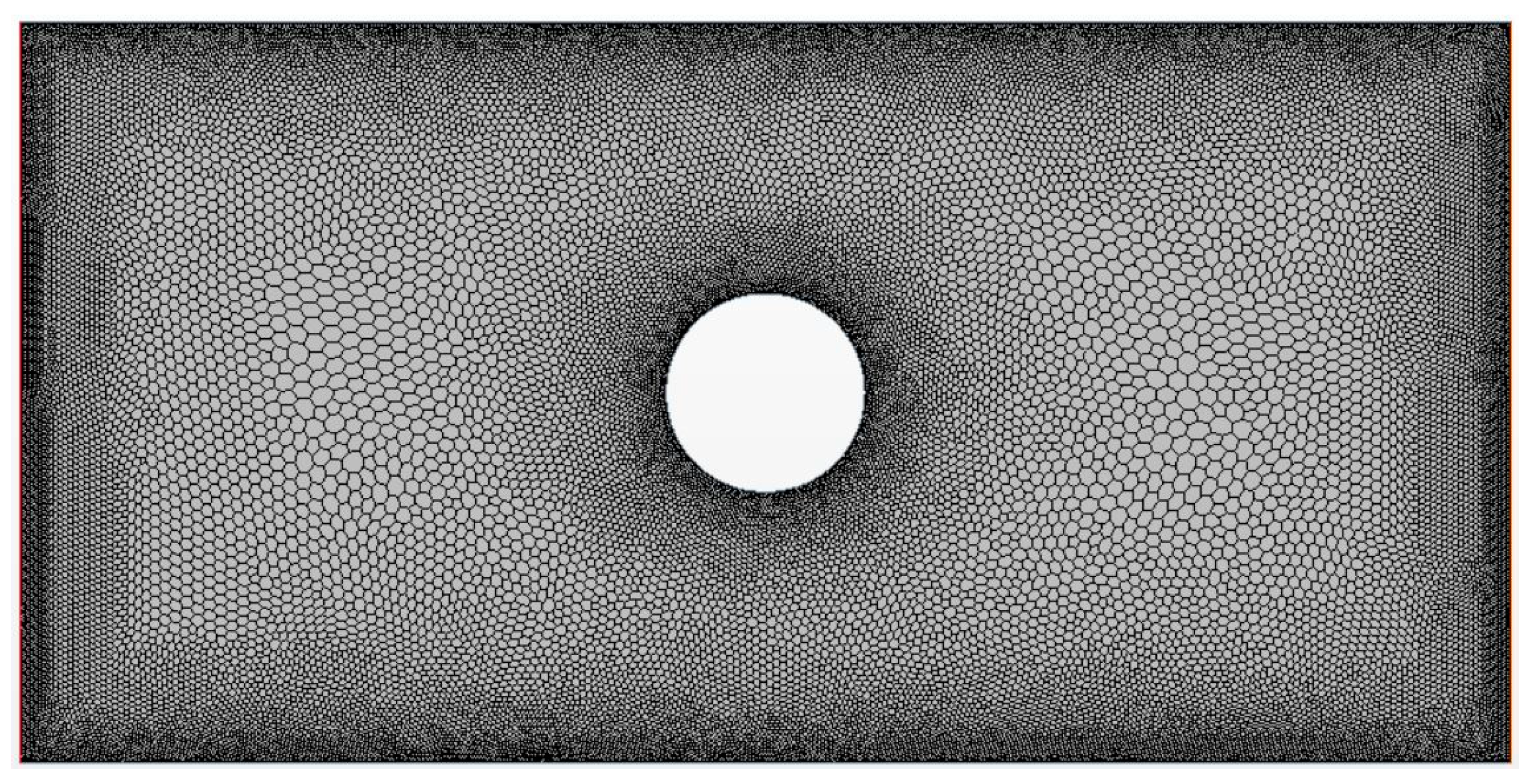
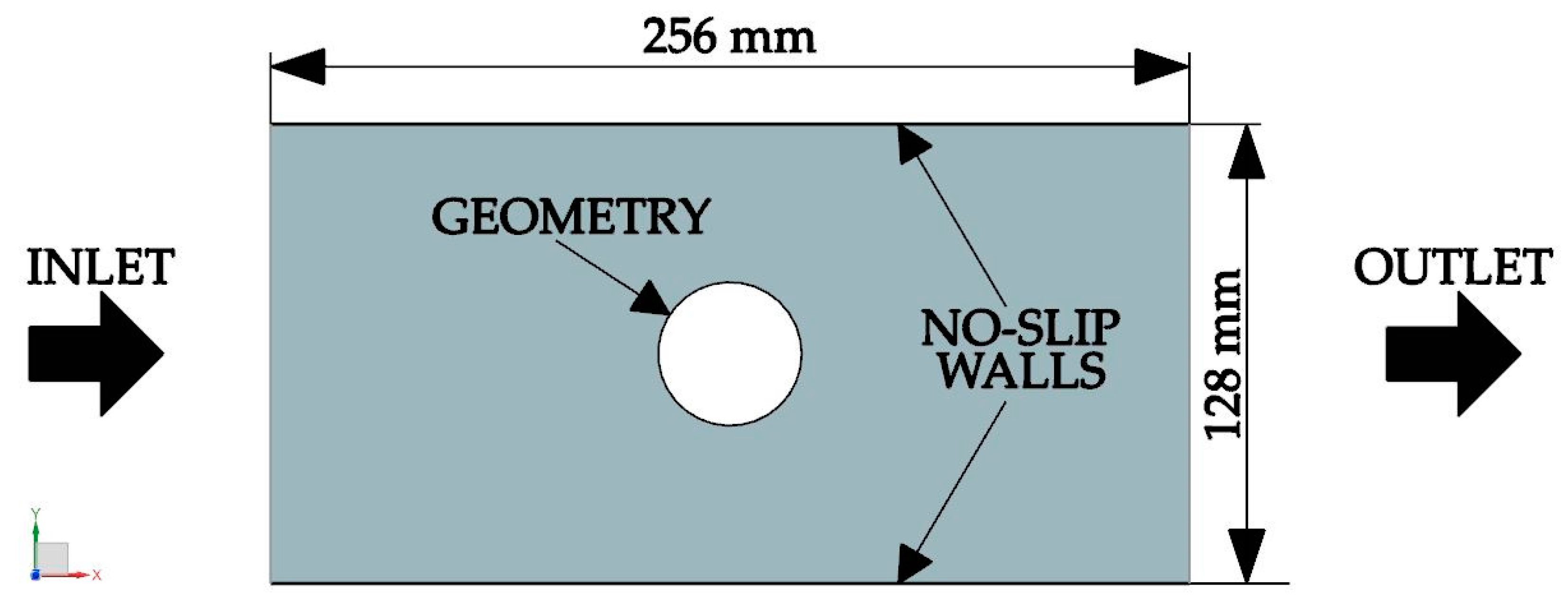
2.1. CFD Setup
2.2. Convolutional Neural Network
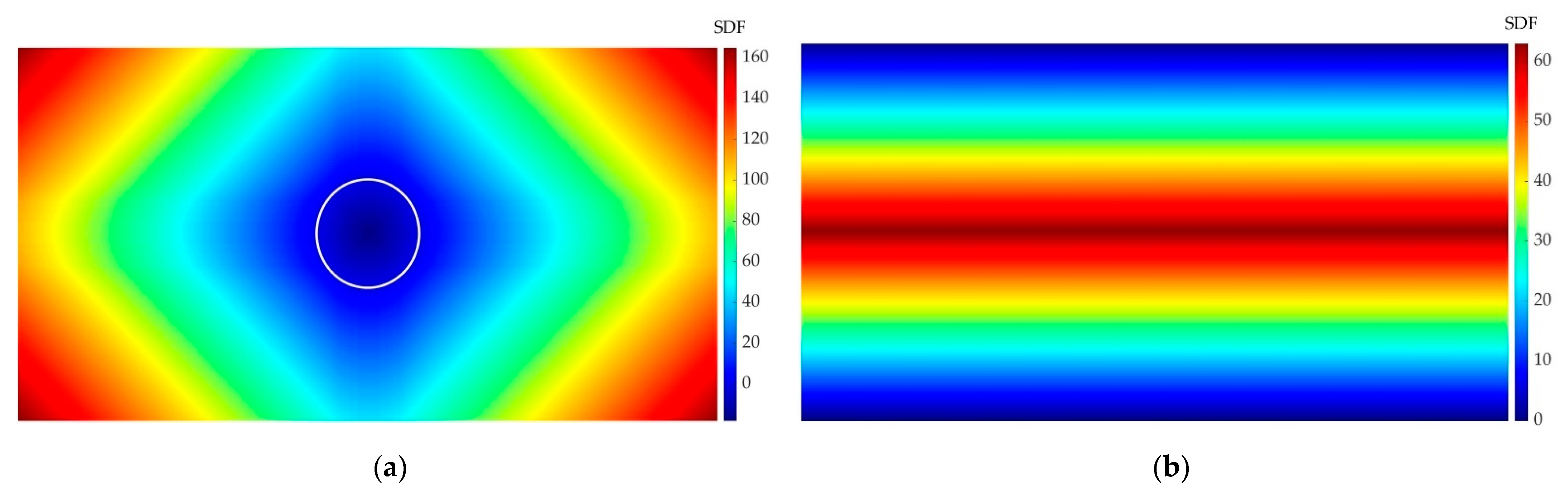
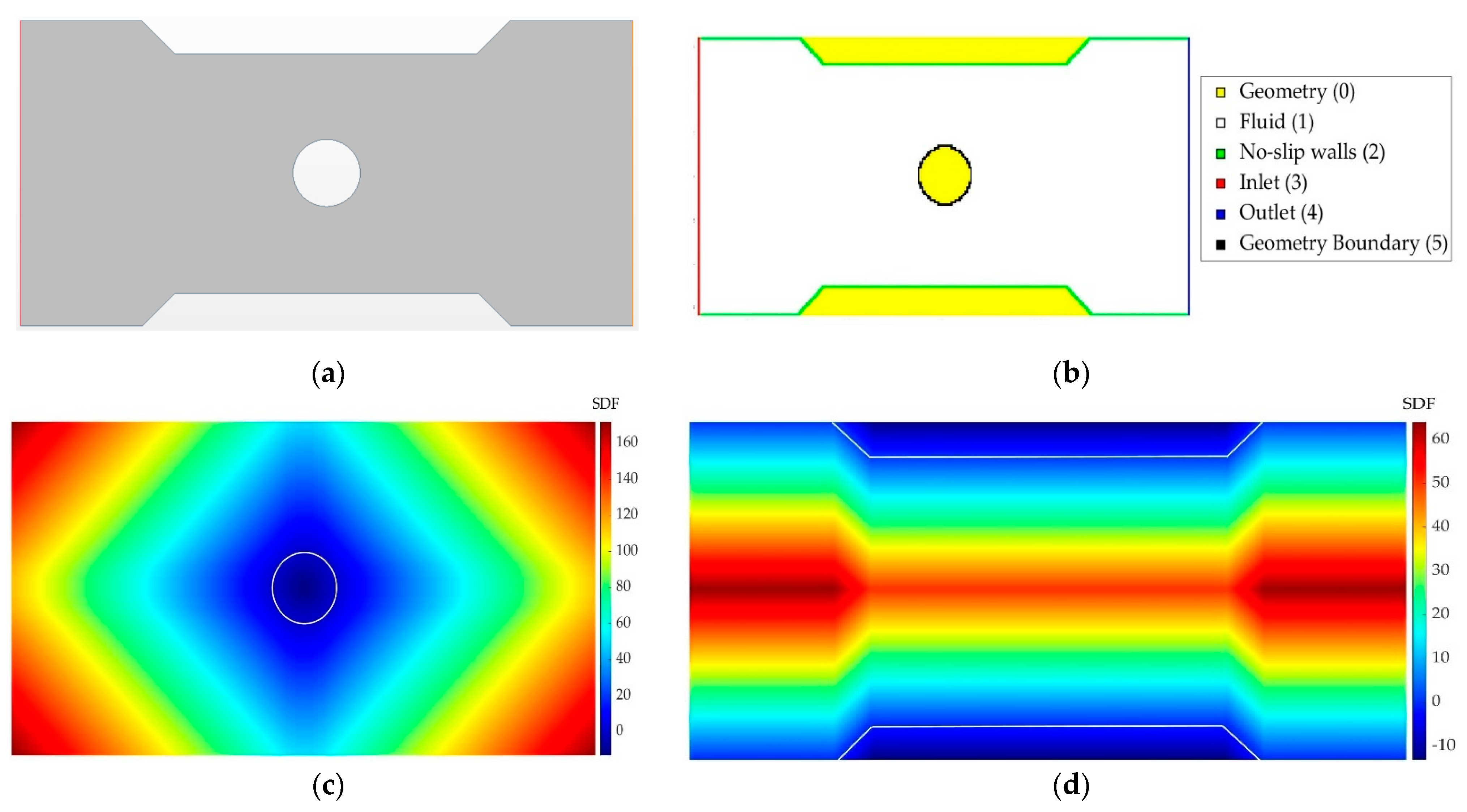
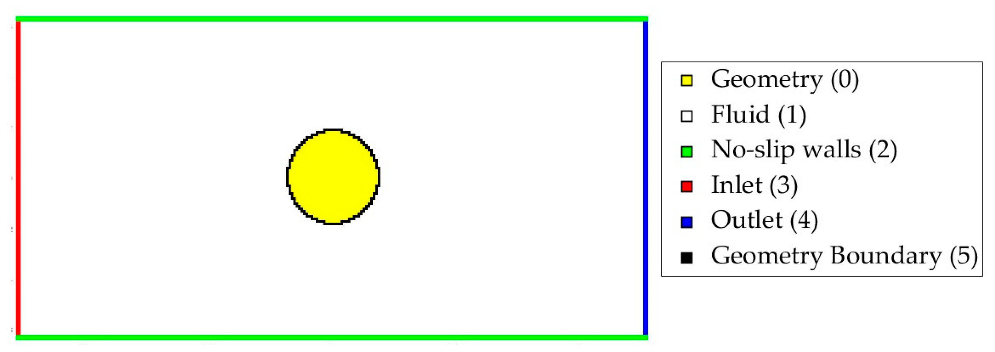
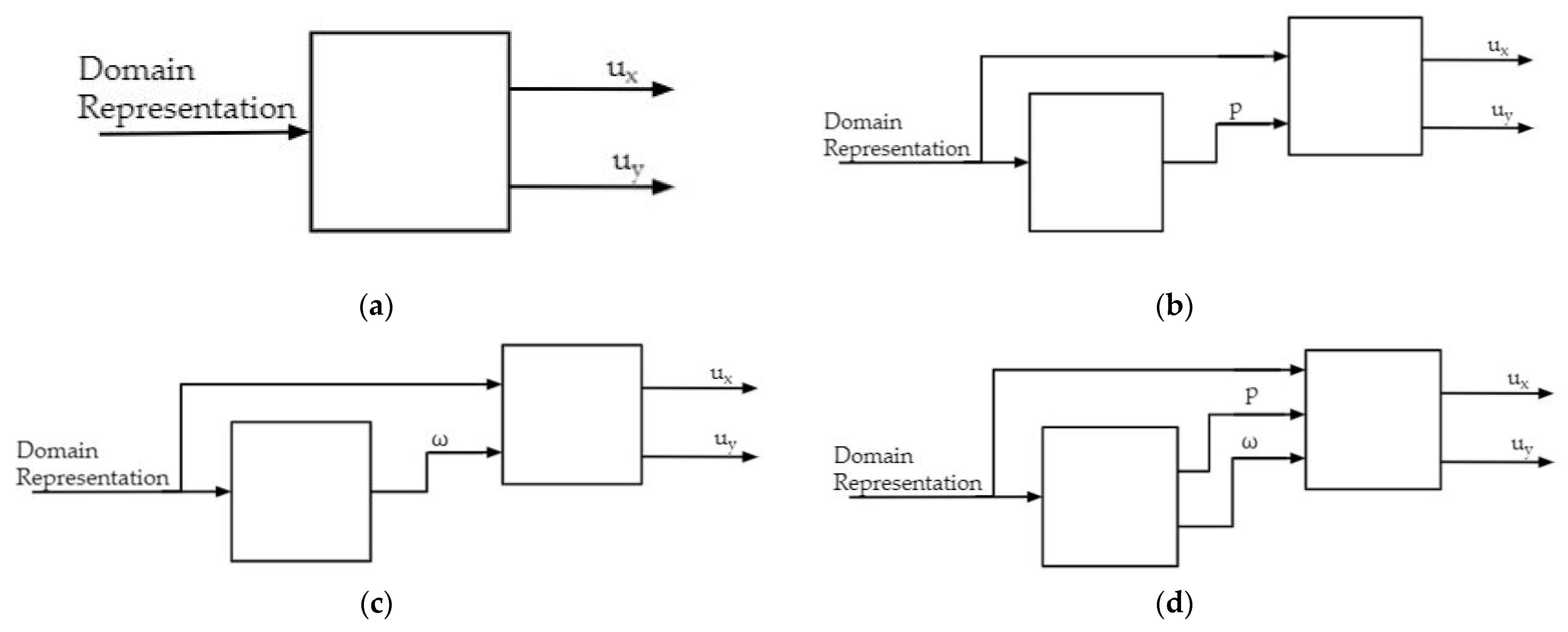
2.2.1. Domain Representation
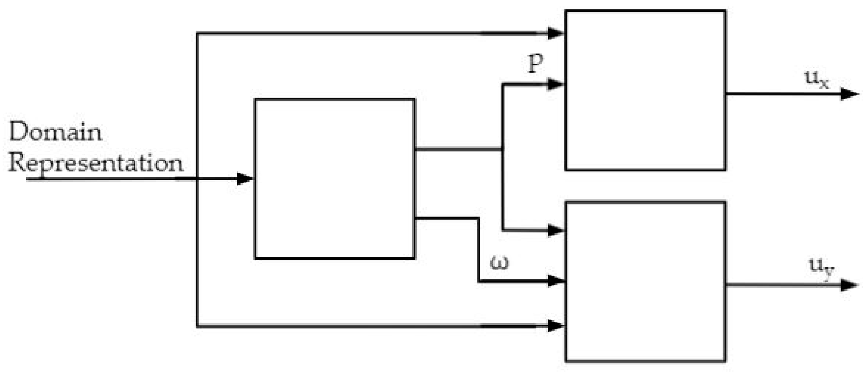
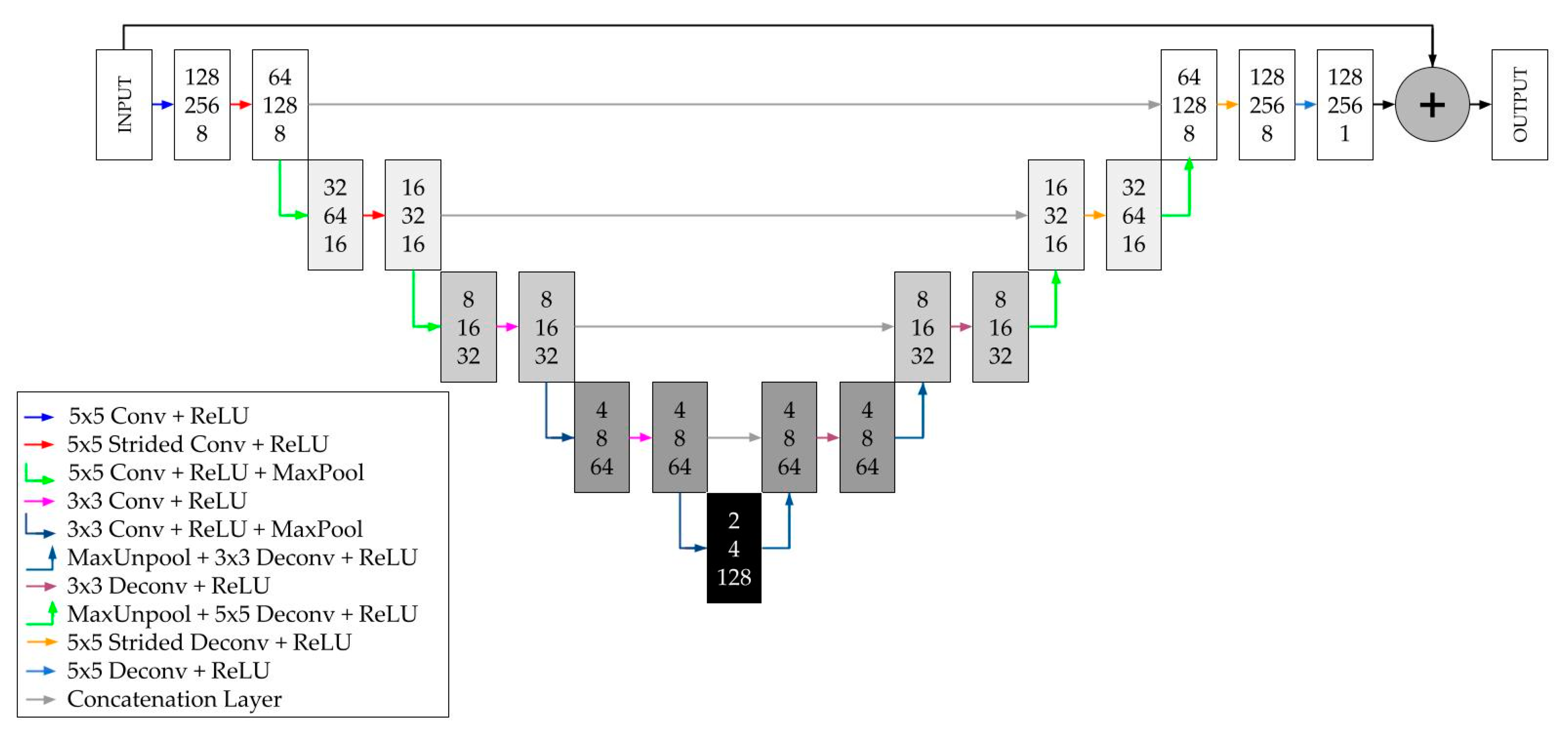
2.2.2. Neural Network Architecture
2.2.3. Neural Network Configurations
3. Results and Discussion
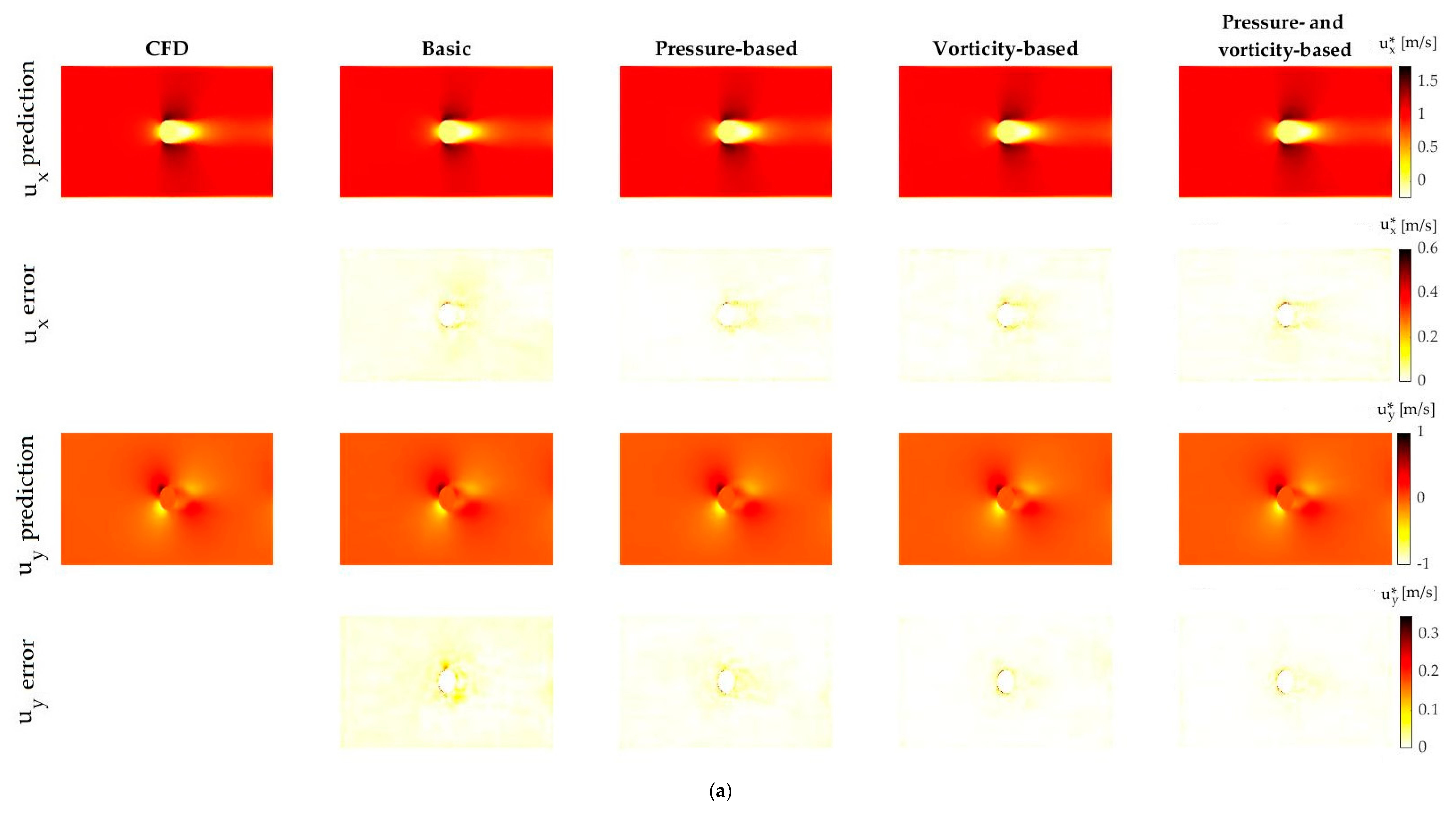
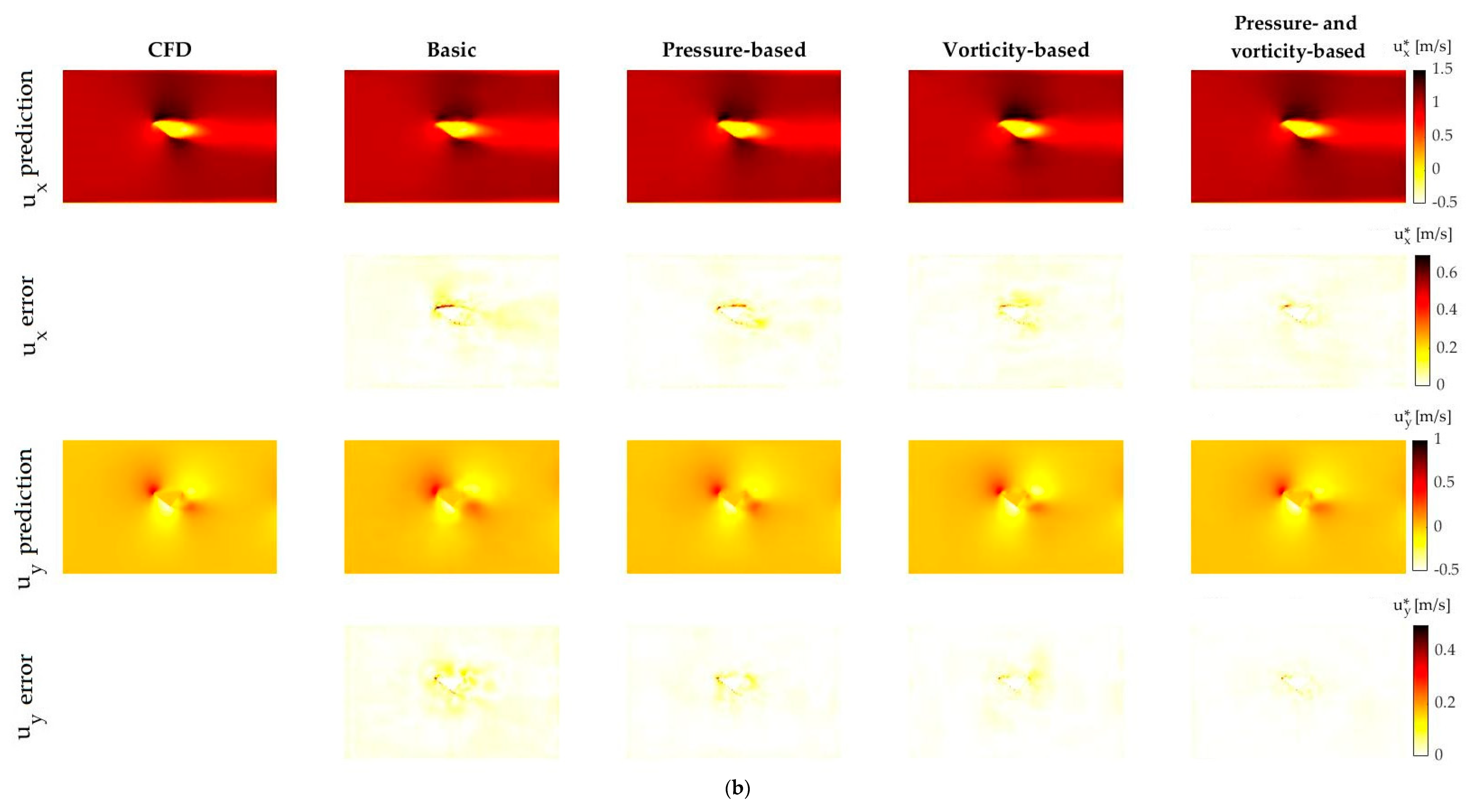
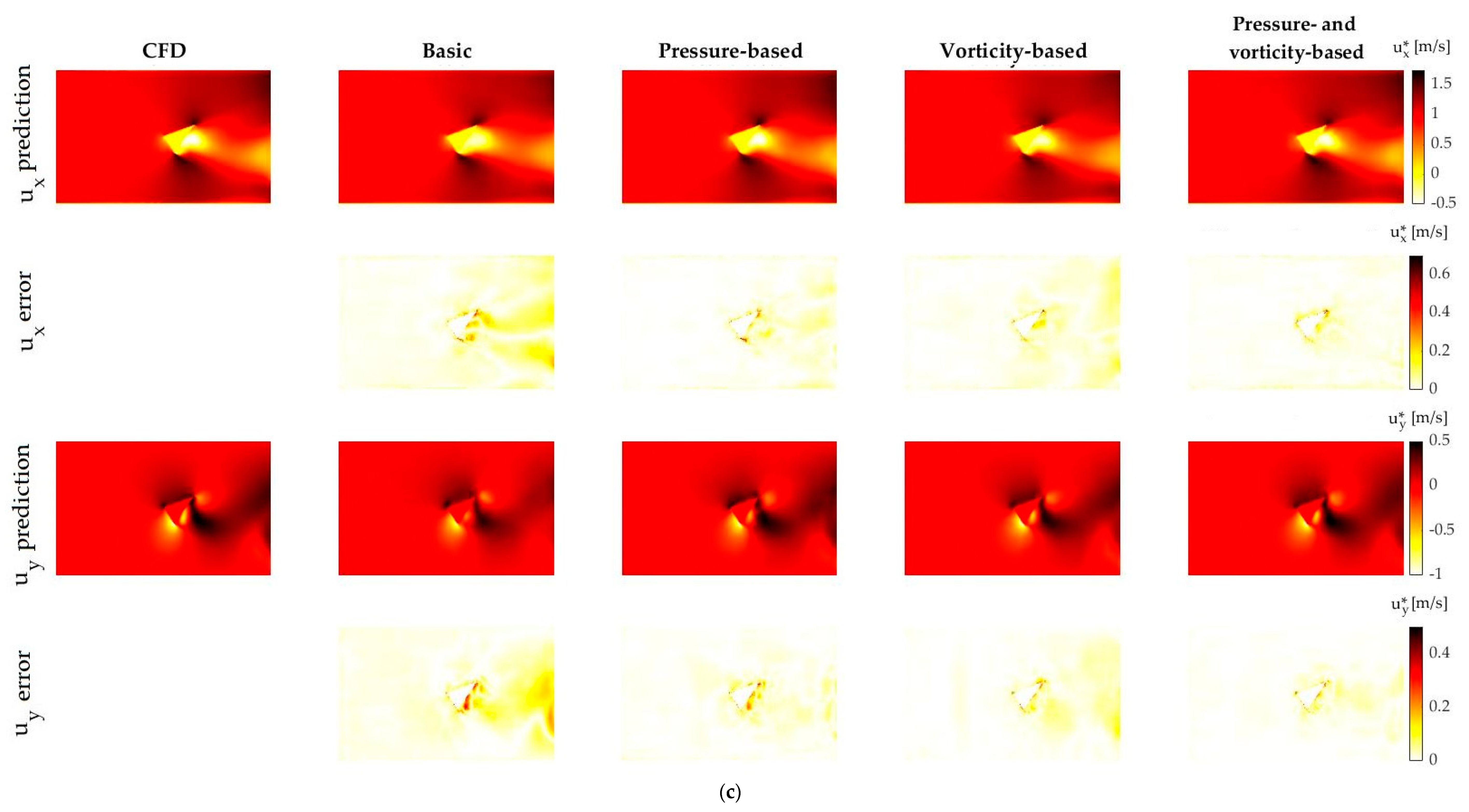
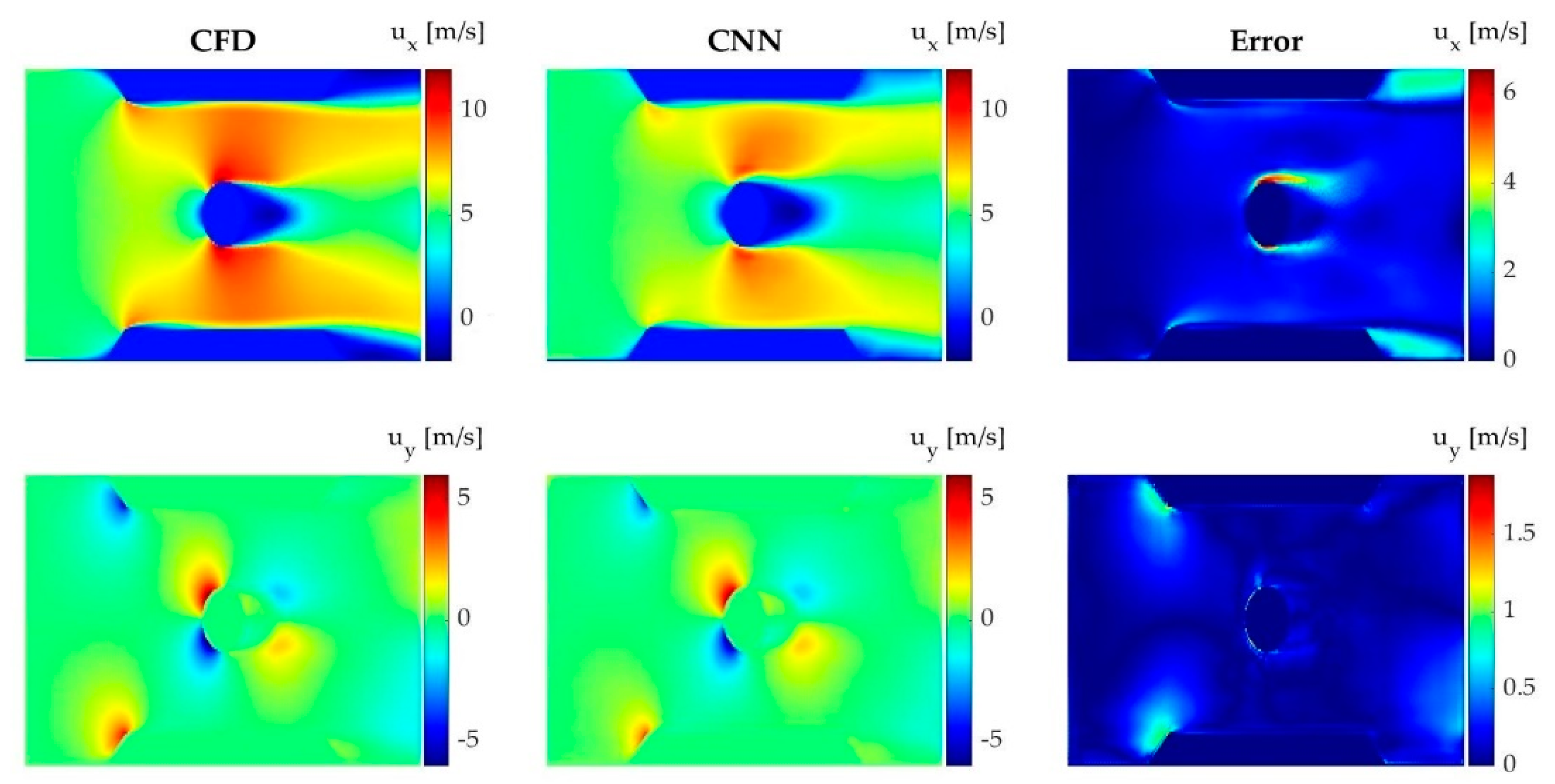
3.1. Qualitative Study
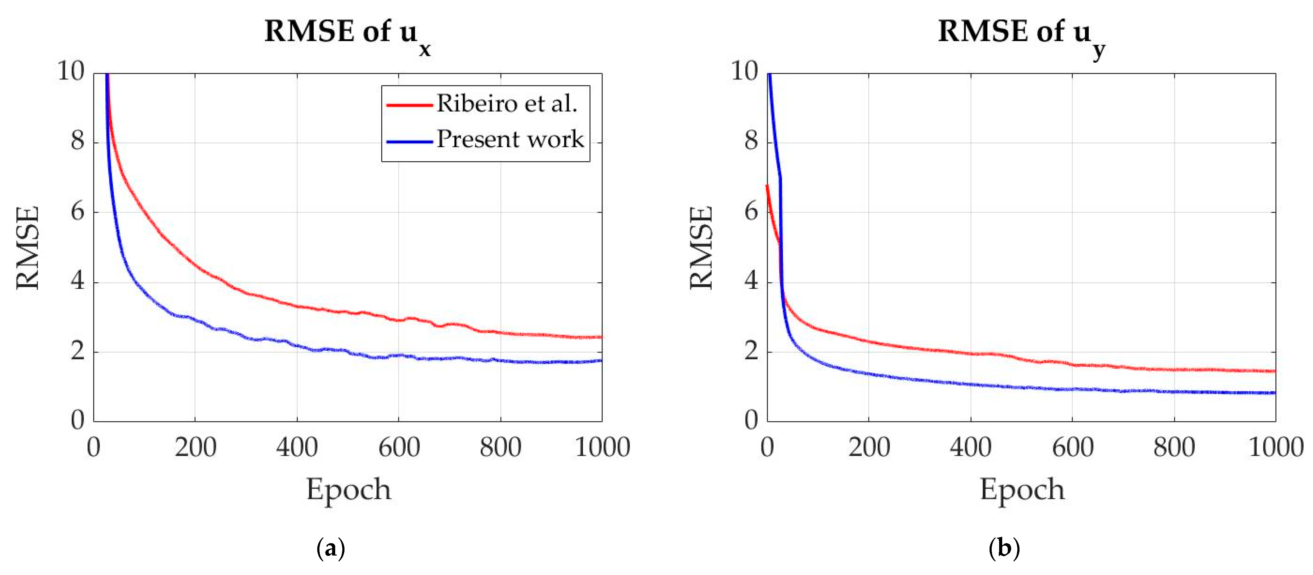
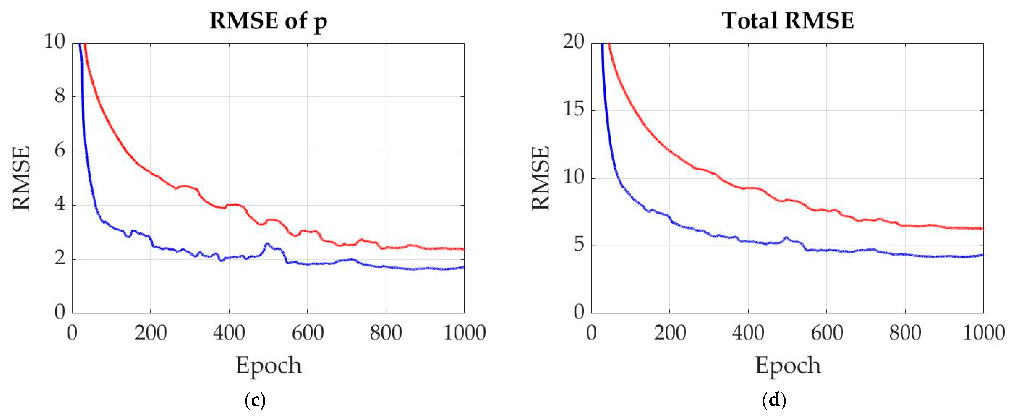
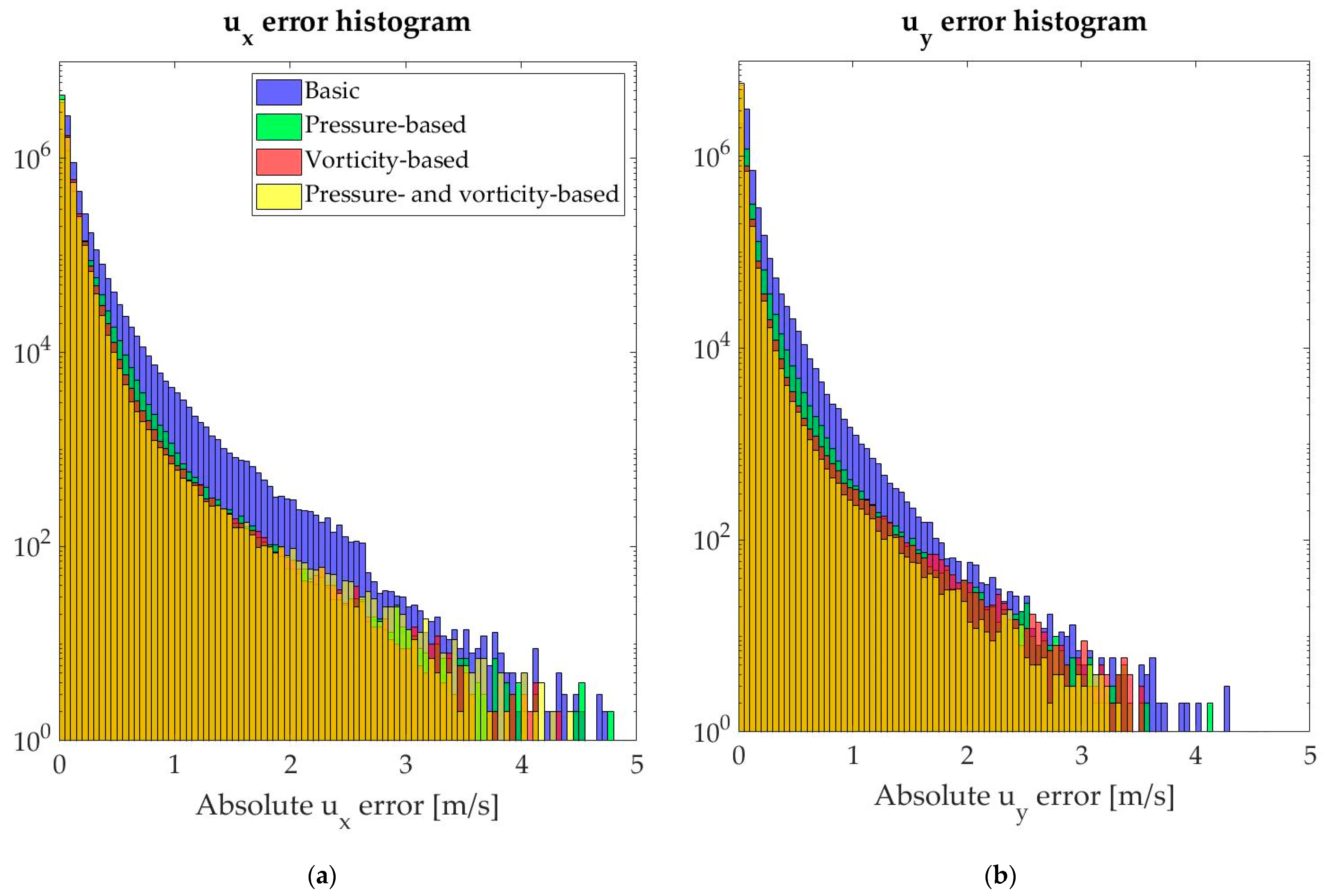
3.2. Quantitative Study
3.3. Performance Analysis
4. Network Testing
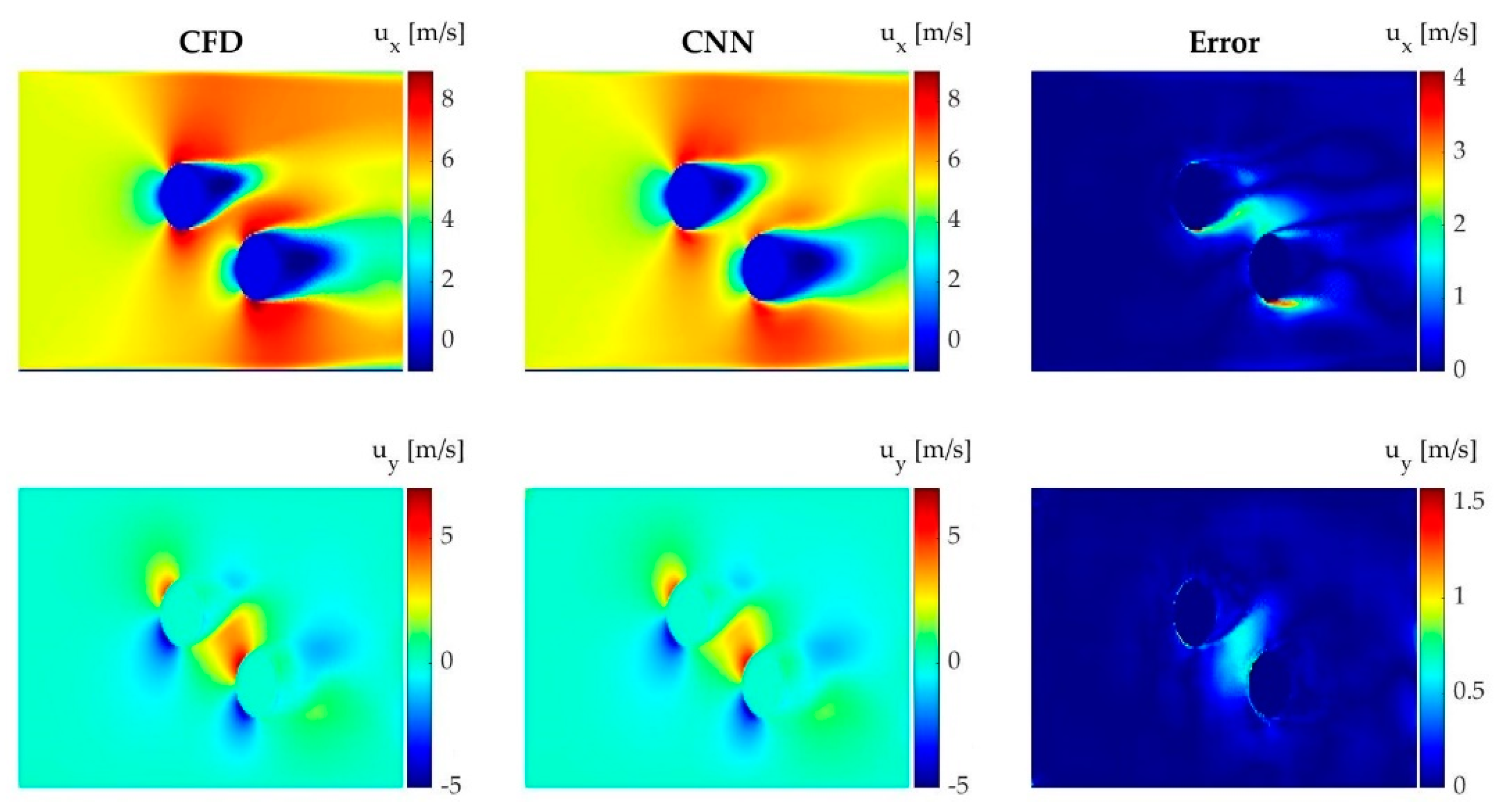
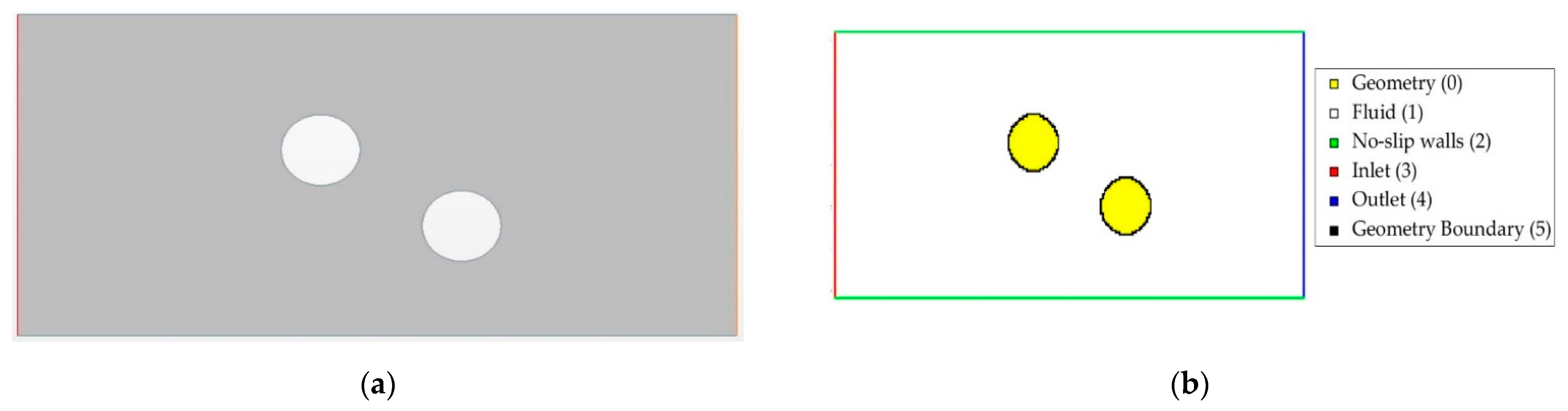
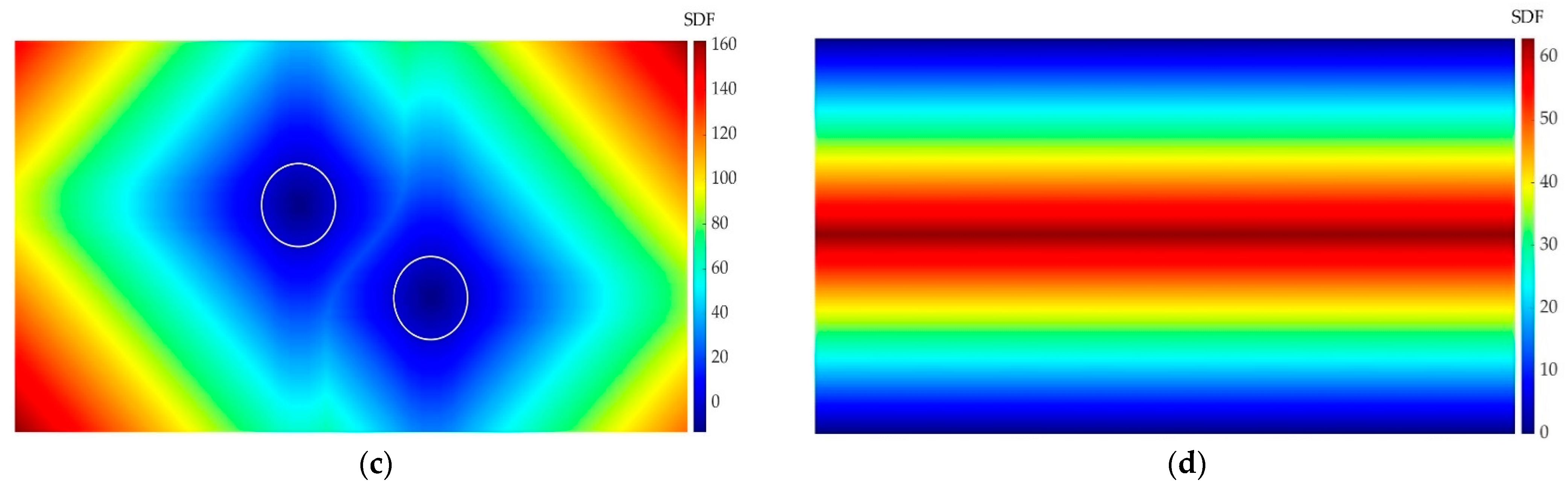
4.1. Multiple Objects
4.2. Different Channel
5. Conclusions
Author Contributions
Funding
Institutional Review Board Statement
Informed Consent Statement
Data Availability Statement
Acknowledgments
Conflicts of Interest
Nomenclature
| Definition | |
| ANN | Artificial Neural Network |
| CFD | Computational Fluid Dynamics |
| CNN | Convolutional Neural Network |
| DL | Deep Learning |
| DML | Deep Metric Learning |
| DNN | Deep Neural Network |
| DNS | Direct Numerical Simulation |
| FRC | Flow Region Channel |
| GAN | Generative Adversarial Network |
| LES | Large Eddy Simulation |
| RANS | Reynolds-Averaged Navier-Stokes |
| ReLU | Rectifier Linear Unit |
| RMSE | Root-Mean-Square Error |
| SDF | Signed Distance Function |
| * | Dimensionless value |
| ‘ | Value ranged between [0, 1] |
| Mean value | |
| a | Characteristic length of the geometry |
| b | Characteristic length of the geometry |
| c | Speed of sound |
| Model coefficient | |
| Model coefficient | |
| Model coefficient | |
| Model coefficient | |
| Model coefficient | |
| γ | Characteristic angle of the geometry |
| Compressibility modification | |
| ε | Dissipation rate |
| Resultant of body forces | |
| Gravitational vector | |
| Buoyancy production | |
| Turbulent production | |
| I | Identity tensor |
| k | Turbulent kinetic energy |
| L | Projection of the geometry on the direction of the flow |
| Fluid density | |
| Pressure | |
| p | Order of accuracy (in General Richardson Extrapolation) |
| Production term | |
| Production term | |
| Turbulent Prandtl number | |
| R | Convergence condition (in General Richardson Extrapolation) |
| Re | Reynolds number |
| RE | Estimated value (in General Richardson Extrapolation) |
| Model coefficient | |
| Model coefficient | |
| T | Viscous stress tensor |
| Mean temperature | |
| μ | Fluid dynamic viscosity |
| Turbulent viscosity | |
| Horizontal velocity | |
| Vertical velocity | |
| Vorticity | |
| Zero level set (in SDF) |
References
- Ray, D.; Hesthaven, J.S. An artificial neural network as a troubled-cell indicator. J. Comput. Phys. 2018, 367, 166–191. [Google Scholar] [CrossRef] [Green Version]
- Liu, Y.; Lu, Y.; Wang, Y.; Sun, D.; Deng, L.; Wan, Y.; Wang, F. Key time steps selection for CFD data based on deep metric learning. Comput. Fluids 2019, 195, 104318. [Google Scholar] [CrossRef]
- Bao, H.; Feng, J.; Dinh, N.; Zhang, H. Computationally efficient CFD prediction of bubbly flow using physics-guided deep learning. Int. J. Multiph. Flow 2020, 131, 103378. [Google Scholar] [CrossRef]
- Hanna, B.N.; Dinh, N.T.; Youngblood, R.W.; Bolotnov, I.A. Coarse-Grid Computational Fluid Dynamic (CG-CFD) Error Prediction Using Machine Learning. arXiv 2017, arXiv:171009105. [Google Scholar]
- Yan, X.; Zhu, J.; Kuang, M.; Wang, X. Aerodynamic shape optimization using a novel optimizer based on machine learning techniques. Aerosp. Sci. Technol. 2019, 86, 826–835. [Google Scholar] [CrossRef]
- Zhang, X.; Xie, F.; Ji, T.; Zhu, Z.; Zheng, Y. Multi-Fidelity deep neural network surrogate model for aerodynamic shape optimization. Comput. Methods Appl. Mech. Eng. 2021, 373, 113485. [Google Scholar] [CrossRef]
- Tao, J.; Sun, G. Application of deep learning based multi-fidelity surrogate model to robust aerodynamic design optimization. Aerosp. Sci. Technol. 2019, 92, 722–737. [Google Scholar] [CrossRef]
- Guo, X.; Li, W.; Iorio, F. Convolutional neural networks for steady flow approximation. In Proceedings of the 22nd ACM SIGKDD International Conference on Knowledge Discovery and Data Mining, San Francisco, CA, USA, 13 August 2016; pp. 481–490. [Google Scholar]
- Ling, J.; Kurzawski, A.; Templeton, J. Reynolds averaged turbulence modelling using deep neural networks with embedded invariance. J. Fluid Mech. 2016, 807, 155–166. [Google Scholar] [CrossRef]
- Lee, S.; You, D. Prediction of laminar vortex shedding over a cylinder using deep learning. arXiv 2017, arXiv:1712.07854. [Google Scholar]
- Liu, Y.; Lu, Y.; Wang, Y.; Sun, D.; Deng, L.; Wang, F.; Lei, Y. A CNN-based shock detection method in flow visualization. Comput. Fluids 2019, 184, 1–9. [Google Scholar] [CrossRef]
- Deng, L.; Wang, Y.; Liu, Y.; Wang, F.; Li, S.; Liu, J. A CNN-based vortex identification method. J. Vis. 2019, 22, 65–78. [Google Scholar] [CrossRef]
- Ribeiro, M.D.; Rehman, A.; Ahmed, S.; Dengel, A. DeepCFD: Efficient steady-state laminar flow approximation with deep convolutional neural networks. arXiv 2020, arXiv:2004.08826. [Google Scholar]
- Kashefi, A.; Rempe, D.; Guibas, L.J. A Point-cloud deep learning framework for prediction of fluid flow fields on irregular geometries. arXiv 2020, arXiv:2010.09469. [Google Scholar]
- Nowruzi, H.; Ghassemi, H.; Ghiasi, M. Performance predicting of 2D and 3D submerged hydrofoils using CFD and ANNs. J. Mar. Sci. Technol. 2017, 22, 710–733. [Google Scholar] [CrossRef]
- Mohan, A.; Daniel, D.; Chertkov, M.; Livescu, D. Compressed convolutional LSTM: An efficient deep learning framework to model high fidelity 3D turbulence. arXiv 2019, arXiv:1903.00033. [Google Scholar]
- Fang, R.; Sondak, D.; Protopapas, P.; Succi, S. Deep learning for turbulent channel flow. arXiv 2018, arXiv:1812.02241. [Google Scholar]
- Thuerey, N.; Weißenow, K.; Prantl, L.; Hu, X. Deep learning methods for reynolds-averaged navier–stokes simulations of airfoil flows. AIAA J. 2020, 58, 25–36. [Google Scholar] [CrossRef]
- Sun, L.; Gao, H.; Pan, S.; Wang, J.-X. Surrogate modeling for fluid flows based on physics-constrained deep learning without simulation data. Comput. Methods Appl. Mech. Eng. 2020, 361, 112732. [Google Scholar] [CrossRef] [Green Version]
- STAR-CCM+ V2019.1. Available online: https://www.plm.automation.siemens.com/ (accessed on 2 June 2020).
- Richardson, L.F.; Gaunt, J.A. The deferred approach to the limit. Philos. Trans. R. Soc. Lond. Ser. A Contain. Pap. Math. Phys. Character 1927, 226, 299–361. [Google Scholar] [CrossRef]
- Roshko, A. Vortex Shedding from Circular Cylinder at Low Reynolds Number; Cambridge University Press: Cambridge, UK, 1954. [Google Scholar]
- Shih, T.-H.; Liou, W.W.; Shabbir, A.; Yang, Z.; Zhu, J. A new k-ε Eddy viscosity model for high Reynolds number turbulent flows: Model development and validation. Computers Fluids 1995, 24, 227–238. [Google Scholar] [CrossRef]
- Ronneberger, O.; Fischer, P.; Brox, T. U-net: Convolutional networks for biomedical image segmentation. In Proceedings of the Medical Image Computing and Computer-Assisted Intervention—MICCAI 2015, Munich, Germany, 5–9 October 2015; Navab, N., Hornegger, J., Wells, W.M., Frangi, A.F., Eds.; Springer: Cham, Switzerland, 2015; pp. 234–241. [Google Scholar]
- MATLAB. Available online: https://es.mathworks.com/products/matlab.html (accessed on 9 June 2021).
- Deep Learning Toolbox. Available online: https://es.mathworks.com/products/deep-learning.html (accessed on 3 July 2021).
- Kingma, D.P.; Ba, J. Adam: A Method for Stochastic Optimization. arXiv 2017, arXiv:1412.6980. [Google Scholar]


| Shape | Sketch | Orientation | Scale | Number of Data |
|---|---|---|---|---|
| Circle |  | - | a = 0.02 m, 0.022 m, …, 0.04 m | 11 |
| Equilateral triangle |  | 0°, 3°, …, 177° | a = 0.02 m | 60 |
| Square |  | 0°, 3°, …, 87° | a = 0.02 m | 30 |
| Equilateral pentagon |  | 0°, 3°, …, 69° | a = 0.02 m | 24 |
| Equilateral hexagon |  | 0°, 3°, …, 57° | a = 0.02 m | 20 |
| Ellipse |  | 0°, 3°, …, 177° | a = 0.02 m; b/a = 1.1, 1.2, …, 2 | 600 |
| Rectangle |  | 0°, 3°, …, 177° | a = 0.02 m; b/a = 1.1, 1.2, …, 2 | 600 |
| Triangle |  | 0°, 3°, …, 357° | a = 0.01 m; b/a = 1.5, 1.75; γ = 40°, 60°, 80° | 720 |
| Mesh Resolution | Richardson Extrapolation | Experimental | ||||
|---|---|---|---|---|---|---|
| Coarse | Medium | Fine | RE | p | R | |
| 0.796 | 0.835 | 0.858 | 0.907 | 0.681 | 0.566 | 0.91 |
| Structure | ||
|---|---|---|
| Basic | 0.1145 | 0.0851 |
| Pressure-based | 0.0619 | 0.0466 |
| Vorticity-based | 0.067 | 0.0331 |
| Pressure- and vorticity-based | 0.0636 | 0.0302 |
| Method | Time (s) | Speedup |
|---|---|---|
| CFD | 23,053.2 | - |
| Basic | 21.4 | 1077.25 |
| Pressure-based | 27.35 | 842.9 |
| Vorticity-based | 24.01 | 960.15 |
| Pressure- and vorticity-based | 28.53 | 808.03 |
Publisher’s Note: MDPI stays neutral with regard to jurisdictional claims in published maps and institutional affiliations. |
© 2021 by the authors. Licensee MDPI, Basel, Switzerland. This article is an open access article distributed under the terms and conditions of the Creative Commons Attribution (CC BY) license (https://creativecommons.org/licenses/by/4.0/).
Share and Cite
Portal-Porras, K.; Fernandez-Gamiz, U.; Ugarte-Anero, A.; Zulueta, E.; Zulueta, A. Alternative Artificial Neural Network Structures for Turbulent Flow Velocity Field Prediction. Mathematics 2021, 9, 1939. https://doi.org/10.3390/math9161939
Portal-Porras K, Fernandez-Gamiz U, Ugarte-Anero A, Zulueta E, Zulueta A. Alternative Artificial Neural Network Structures for Turbulent Flow Velocity Field Prediction. Mathematics. 2021; 9(16):1939. https://doi.org/10.3390/math9161939
Chicago/Turabian StylePortal-Porras, Koldo, Unai Fernandez-Gamiz, Ainara Ugarte-Anero, Ekaitz Zulueta, and Asier Zulueta. 2021. "Alternative Artificial Neural Network Structures for Turbulent Flow Velocity Field Prediction" Mathematics 9, no. 16: 1939. https://doi.org/10.3390/math9161939
APA StylePortal-Porras, K., Fernandez-Gamiz, U., Ugarte-Anero, A., Zulueta, E., & Zulueta, A. (2021). Alternative Artificial Neural Network Structures for Turbulent Flow Velocity Field Prediction. Mathematics, 9(16), 1939. https://doi.org/10.3390/math9161939