MMAP/(PH,PH)/1 Queue with Priority Loss through Feedback

Abstract

In this paper, we consider two single server queueing systems to which customers of two distinct priorities ($P_1$ and $P_2$) arrive according to a Marked Markovian arrival process (MMAP). They are served according to two distinct phase type distributions. The probability of a $P_1$ customer to feedback is $\theta$ on completion of his service. The feedback ($P_1$) customers, as well as $P_2$ customers, join the low priority queue. Low priority ($P_2$) customers are taken for service from the head of the line whenever the $P_1$ queue is found to be empty at the service completion epoch. We assume a finite waiting space for $P_1$ customers and infinite waiting space for $P_2$ customers. Two models are discussed in this paper. In model I, we assume that the service of $P_2$ customers is according to a non-preemptive service discipline and in model II, the $P_2$ customers service follow a preemptive policy. No feedback is permitted to customers in the $P_2$ line. In the steady state these two models are compared through numerical experiments which reveal their respective performance characteristics.

1. Introduction

In this paper, we discuss two queueing models arising due to feedback of customers from a high priority queue ($P_1$ queue) joining a lower priority queue ($P_2$ queue), in a single server queueing system. The $P_1$ queue is of finite capacity whereas the $P_2$ queue has unlimited capacity. Immediately after service completion high-priority customers tend to provide feedback on the service again. The probability for feedback at a service completion epoch is $\theta$ which is independent of the feedback by other customers and also the number of customers in the system. However, they are to join a low-priority $P_2$ queue. In addition to this stream of customers in the $P_2$ queue, customers belonging to such class from outside also join that queue. The two models considered are the preemptive and non-preemptive services of $P_2$ customers. The flow of customers constitutes a Marked Markovian arrival process. $P_1$ and $P_2$ customers have service times following two distinct and mutually independent phase type distributions.

Because some abbreviations appear, mostly in this section, we introduce them at this stage for easy reading.

• MMAP: Marked Markovian Arrival Process;
• MMPP: Markov Modulated Poisson Process;
• FBQ: Feedback Queues;
• IFBQ: Instantaneous Feed Back Queue;
• DFBQ: Delayed Feed Back Queue;
• LIQBD: Level Independent Quasi-Birth-and-Death;
• WV: Working Vacations;
• PU: Primary Users;
• SU: Secondary Users;

In addition to introducing some new notions in feedback and priority queues, this paper extends earlier work to a much more general framework. The salient features of the present paper are:

• It brings down the priority of customers when customers, after first service, feedback to the system. Thus it combines feedback and priority to open a new direction of the investigation.
• Because the customers who feedback join a new queue, our model provides the best way to identify such customers, provided low priority customers are not admitted to the system. In Krishnamoorthy and Manjunath [1] no entry of external customers to the low priority queue, was considered. Thus this paper is a further extension of [1]. Prior to introducing this type of feedback of customers, only two types of feedback were considered in the literature: (i) feedback to the tail end of the queue and (ii) continue service as a feedback customer on completion of the first service. Thus it is hard to identify feedback customers, if at all any, in these cases. In addition, if we allow more than two priorities, then more than one feedback can be allowed to each customer; such feedback customers are directed to the immediately low priority queue. Thus the problems discussed in this paper have several practical utilities.
• This has certain advantages, which include minimizing unnecessarily bothering the server with questions that were clarified in the earlier rounds of service. This feat is achieved through feedback customers being downgraded in their priority.
• The low priority queue accommodates both external customers (of lower priority) and feedback customers from the first priority queue. Though in the literature there is just one paper (see Krishnamoorthy and Manjunath [1]) that considers customer feedback-generated low priority queue, it does not consider external customers of low priority, joining the feedback-driven low priority queue. Besides, in [1] only a very simple case of exponentially distributed service time and Poisson arrival of Priority 1 customer to the system, are considered. In contrast, in this paper MMAP arrival of customers and distinct phase-type distributed service time for the two types of customers, are considered.
• In addition to the above indicated features, a number of extensions of this work is also indicated in the concluding section.

Before going to further details of the paper, we provide literature review on the two topics—feedback and priority queue.

1.1. Literature Review of Feedback Queues

FBQ are extensively discussed in the queueing literature. They are adequate mathematical models of computer communication networks, manufacturing systems, inventory management processes, and many other systems in which a few served customers may require re-servicing for some reason. Indeed, in information transmission systems, erroneously transmitted data (packets, frames, etc.) are re-transmitted; defective items produced during a manufacturing process have to be re-processed, and so on.

Although these systems are widely used in real life, they have not been sufficiently studied for a long time. Such models were first introduced in [2,3]. After these pioneering works, researchers again did not pay attention to them for a long time. Only in the last three decades have such systems been intensively studied by various authors.

In the class of FBQ, it is necessary to distinguish two subclasses: IFBQ, where a return occurs immediately after the service is completed, and DFBQ, in which a request by a customer who was already served out occurs after the elapse of a certain amount of time.

In [4,5], detailed reviews of work conducted on FBQ until 2015 are provided. Therefore, we restrict ourselves to those published from 2016 onwards.

Note that in most of the work reported on FBQ, no separate queue for such customers is considered. In such kinds of systems, it is very hard to control the loss probabilities of primary and feedback calls. To reduce the loss probabilities of calls, sometimes an orbit(s) for both kind of calls is organized. In recent years, models of feedback queues with reliable and unreliable server subject to various schemes of breakdowns and repairs, have been investigated (see Rajadura et al. [6], Ke et al. [7], Singh et al. [8], Jailaxmi et al. [9], Chang et al. [10], Chang et al. [11], Madheswari et al. [12], Melikov et al. [13], Jain and Kaur [14]). The above-mentioned authors study the IFBQ model with buffers as indicated in the respective papers.

In VijayaLaxmi et al.’s work [15], the model of a feedback M/M/1 queueing system with correlated reneging and WV is examined. To compute the long run system state distribution of the resulting three-dimensional Markov chain, a matrix-geometric method is employed. Using this, several system performance measures are calculated and an optimization problem discussed.

Bouchentouf et al. [16] consider an M/M/1/N feedback queue with server vacation, balking, reneging and holding those reneged customers to the system.

To study a single channel cognitive radio network with a slotted time structure, Zhao and Yue [17] perform analysis and optimization of the system with a finite primary buffer and a probabilistic returning scheme. PU packets can always be transmitted on the channel because the channel is authorized to do so. However, SU packets that access the system, are transmitted opportunistically. To reduce packet loss probability, separate finite buffers are organized for both kinds of users. It is assumed that PU packets have preemptive priority over SU packets, i.e., a PU packet can interrupt an SU packet’s transmission. A feedback scheme is accepted for interrupted SU packets, i.e., it is assumed that an interrupted SU packet, in accordance with the Bernoulli scheme, can either be admitted through the SU buffer and wait for the next transmission or be forced to leave the system.

Melikov et al. [13] analyze an IFBQ with heterogeneous servers and MMPP flow. Primary calls are served on a high-speed server. On completion of service, each call either leaves the system or asks for repeated service according to a Bernoulli scheme. Such calls, on completion of service by a slow server, leave the system or return for re-servicing according to the Bernoulli scheme. With the arrival of a primary call, if the queue length of such calls exceeds a certain threshold value and the slow server is free, then the incoming primary call is either directed to the slow server or joins its queue according to the prescribed Bernoulli scheme. Algorithms for calculating the steady-state system probabilities approximately are proposed for both finite and infinite capacity systems. Their high accuracy is demonstrated.

Melikov et al. [18] discuss methods to calculate the system state distribution with instantaneous feedback and a varying arrival rates in a Markov model of a servicing system with one server. At a service completion epoch, the customer either leaves the system or immediately returns to receive the service, which is repeated according to a predefined Bernoulli scheme. Prior to a repeated service, a random server switching time is needed. The rate of arrival of external customers depends on whether the server is in operating or switching mode. The condition for ergodicity of this two-dimensional Markov chain is obtained. Further, three methods for studying it are implemented: the method of generating functions, the method of spectral expansion, and the space merging method.

Melikov et al. [19], analyze a multi-channel queuing system with MMPP flow and delayed feedback. After receiving complete service, customers will decide either to feedback with some state-dependent probability or to leave the system forever with complementary probability. Feedback calls organize an orbit of repeated calls. If all channels of the system are busy when a repeated call arrives, then it either leaves the system with some state-dependent probability or with a complementary probability returns to orbit. Methods to calculate the steady-state probabilities of the appropriate three-dimensional Markov chain, as well as some performance measures of the system under consideration are developed.

1.2. Literature Review of Priority Queues

Priority queues were first considered by White and Christie [20] as a queue with interruption of service of low priority customers to provide service to higher priority customers. A priority queue with preemptive service can be regarded as a queue with service interruption. For example, a doctor renders their service to a causality patient urgently by interrupting the present consultation in case it is not critical. Jaiswal [21] is in the preemptive priority queue with resumption of service of the low priority customer and Jaiswal [22] discusses time-dependent solutions in priority queues. Cobham [23] considers a non-preemptive priority queue and derived the expected waiting time in equilibrium. A detailed discussion of development in priority queues until 1968 is given in Jaiswal [24]. More recent developments on priority queues could be found in Takagi [25] and Brodal’s work [26].

Interruption in service due to server failure is discussed extensively in the literature. In the survey paper by Krishnamoorthy et al. [27], an account of various types of server interruptions is provided. This includes interrupting current service to attend higher priority work.

Customer induced service interruption, as coined by Jacob et al. [28], is in contrast to that of interruption due to server failure. This is carried out for the single server case, where customers who experienced interrupted service are given priority over primary customers. Here self-interrupted customer takes an exponentially distributed time to get out of interruption. This is extended to the multi-server case in Krishnamoorthy and Jacob [29]. All underlying distributions (inter-arrival time, service time, inter-interruption time, interruption fixation time) are assumed to be independent exponential random variables. Dudin et al. [30] extend the above case to a Markovian arrival process and phase type service with c servers and negative customers with a few protected service phases.

Lowering of priority of customers in feedback queues is introduced in Krishnamoorthy and Manjunath [1] (see also the Doctoral thesis by Manjunath [31], Chapter 3). Following these works, we assumed that the $P_1$ customers who opt for feedback are allotted low priority and so joins the $P_2$ queue along with those customers who are primary $P_2$ customers.

We can increase the amount of feedback permitted to both classes of customers up to a finite number. This could be achieved by introducing feedback of $P_2$ customers after service, placing them in a queue labeled $P_3$, in which customers of priority 3 join from outside. This can be repeated up to a maximum of K feedback by $P_1$ customers, $K-1$ feedback by $P_2$ customers, and just 1 feedback by $P_K$ customers. If all queues are allowed to have infinite capacity, then the block matrix entries themselves will be of infinite dimensions. In the simple case of Poisson arrivals of external customers to the respective designated queues and exponentially distributed service time, we will be able to derive explicit expressions for system state probability.

Note that the low priority queue(s) is generated by an internal mechanism as well as an external one in the present paper. However, Krishnamoorthy and Manjunath [1] consider only the internal generation of feedback customers. They were able to employ the matrix geometric method, with all queues having infinite capacity because all underlying distributions were exponential. This helped them achieve a very nice structure for the infinitesimal generator of the resulting continuous-time Markov chain. The block matrix entries in the infinitesimal generator are also of infinite dimensions.

Note that the low priority queue(s) are dependent on the higher priority ones also in its evolution. For example, $P_3$ depends on $P_1$ and $P_2$ when we consider at least three distinct priorities. Various feedback policies in different queuing models are studied in the literature (see, for example, [2,32,33,34,35,36,37]). An M/G/1 retrial queue with instantaneous customer feedback is considered by Krishnakumar et al. [38]. In this, the feedback customer joins the tail end of the queue. In [39], Krishnakumar et al. analyze a queue with more than one server; here, it is also assumed that the feedback customer joins the tail end of the queue. A queue with collisions and instantaneous feedback of unsatisfied customers is the theme of discussion in Krishnakumar’s work [40].

Prior to the introduction of a queue generated by feedback customers, the feedback considered fell into two categories: Either the feedback customer joins the tail end of the queue on completion of service so the service is repeated or he occupies the server immediately on completion of the service without joining the queue.In these two cases no separate queue for feedback customers is provided. Further, they have the disadvantage of non-identification of feedback customers. Additionally, note that there may be several feedback customers in the system at a time, some of whom have repeated this several times. In the second case, there is at most one feedback customer at any time in the system. If at all there is one, it is the one undergoing service. In the models that we discuss or in their extension to K feedback, we cannot distinguish feedback customers and primary customers in lower priority queues. However, if we do not allow the external flow of customers to queues, except the feedback customers from the immediate higher priorities, then all customers in the remaining queues are feedback customers. This helps in the control of the number of feedback to be allowed in a service system.

The following explanation gives the motivation behind this paper.

The type of feedback which is introduced here is totally different from those discussed in the literature prior to 2018. The feedback customers considered in this paper are given a lower priority. This is because during a service, for example, purchase of equipment, customers are given detailed explanation about the functioning of the system. After this exercise, a few customers may have the tendency to keep on asking questions about the machinery. This is a big nuisance to big organizations who want this process to be brisk. Thus, those customers who are not satisfied by the first service are directed, immediately after service completion, to the lower priority queue. External customers also join this lower priority queue. Thus, here we notice an interplay between feedback and priority. This also could be seen in offices as follows: suppose a customer requests for a service-this may involve search of previous records. So, after providing him/her with the basic service, the system directs the customer to wait in a separate line, which will be attended when the server becomes free from the first queue.

From the application point of view, we can introduce certain control policies: What is the optimal number of feedback which should be allowed to each priority class when there are at least two priority types considered? This involves the computation of the optimal number of waiting lines that should be provided in the system.

The remaining part of the paper is arranged as follows. Description of model I and its mathematical formulation are given in Section 2. Section 3 provides the ergodicity condition and an algorithm to calculate the steady-state probabilities of the LIQBD associated with the problem. Derivation of waiting time of $P_1$ customers and that of customers in the $P_2$ queue are discussed in Section 4. Additional performance measures are given in Section 5. Model II is described in Section 6 and further its mathematical formulation is also given in that section. A steady-state analysis of that model can be found in Section 7. The analysis of $P_1$ customers’ waiting time and that of customers in the $P_2$ queue appear in Section 8. Additional performance measures are recorded in Section 9. Results of numerical experiments are demonstrated in Section 10.

Following notations are used in what follows:

• $\mathit{e}$: Column vector with all entries 1 of order to be specified.
• ${\mathit{e}}^{\prime }$: Transpose of $\mathit{e}$.
• $CTMC$: Continuous time Markov chain.
• I: Identity matrix of appropriate order.
• $I_a$: Identity matrix of order a.
• ${\mathit{e}}_a\left(b\right)$: Matrix of order $1\times b$ having 1 at position a and 0s’ elsewhere.
• QBD: Quasi-Birth-and-Death
• $d_{ij}^{\left(k\right)}$: entries of $D_k,k=0,1,\mathrm{or}2$
• ${\delta }_l$: $l^{th}$ entry of $D_1\mathit{e}$
• ${\delta }_l^{{}^{\prime }}$: $l^{th}$ entry of $D_2\mathit{e}$

2. Mathematical Formulation of Model I

The mathematical formulation of a single server queue to which arrival of customers form an MMAP with parameters $D_0$, $D_1$, and $D_2$ is considered. The matrix $D_0$ governs transitions without an arrival. $D_1$ and $D_2$ consist of transition rates with the arrival of class 1 (high priority) and that of class 2(low priority) respectively. $D=D_0+D_1+D_2$ is the infinitesimal generator matrix of the arrival process. The matrices are square matrices of order n. Let $\varphi$ denote the stationary probability vector of D. The stationary arrival rate of class $k(k=1,2)$ customers is given by ${\lambda }_k=\varphi D_k\mathit{e}$. Service time of both types of customers is phase-type distributed with representation $(\alpha ,T)$ and $(\beta ,S)$ of orders p and q, respectively. The probability of a $P_1$ customer to feedback is $\theta$ on completion of their service. The feedback ($P_1$) customers, as well as $P_2$ customers, join the low priority queue. Low priority ($P_2$) customers are taken for service from the head of the line whenever the $P_1$ queue is found to be empty at service completion. We assume finite waiting capacity L for $P_1$ customers and infinite waiting space for $P_2$ customers. The service of $P_2$ customers follows a non-preemptive service discipline; that is the arrival of a $P_1$ customer does not interrupt the ongoing service of a $P_2$ customer. No feedback is permitted to customers in the $P_2$ line. It is assumed that the two arrival processes are independent of the service processes.

The QBD Process Associated with Model I

The model described above can be studied as an LIQBD process. First, we introduce the following notations:

• $N_1\left(t\right)$: the number of $P_2$ customers in the system at time t;
• $N_2\left(t\right)$: the number of $P_1$ customers in the system at time t.

At time t:

$$S\left(t\right)=\left\{\begin{array}{cc}0,\hfill & iftheserverisidle\hfill \\ 1,\hfill & if{P}_{1}customerinservice\hfill \\ 2,\hfill & if{P}_{2}customerinservice\hfill \end{array}\right.$$

• $J\left(t\right)$: the phase of the service process when the server is busy;
• $M\left(t\right)$: the phase of the arrival of the customer.

We can verify that $\{(N_1\left(t\right),N_2\left(t\right),S\left(t\right),J\left(t\right),M\left(t\right)):t\ge 0\}$ is an LIQBD with state space

$${\displaystyle \Omega ={\cup }_{i=0}^{\infty }l\left(i\right)}$$

where

• $l\left(0\right)=\{(0,0,0,m)/1\le m\le n\}\cup \{(0,n_2,1,l,m)/1\le n_2\le L;1\le l\le p;1\le m\le n\}\mathrm{and}\mathrm{for}{n}_1\ge 1$,
• $l\left(n_1\right)=\{(n_1,0,2,l,m)/1\le l\le q,1\le m\le n\}\cup \{(n_1,n_2,1,l,m)/1\le n_2\le L;1\le l\le p;1\le m\le n\}\cup \{(n_1,n_2,2,l,m)/1\le n_2\le L;1\le l\le q;1\le m\le n\}$

Note that when $N_1\left(t\right)=N_2\left(t\right)=0$, the server will be idle and so $J\left(t\right)$ need not be considered.

The infinitesimal generator of this CTMC is

$${\mathcal{Q}}_1=\left[\begin{array}{cccc}{B}_0& C_0& & \\ B_1& A_1& A_0& \\ & A_2& A_1& A_0& \\ & & \ddots & \ddots & \ddots \end{array}\right].$$

Here, $B_0$ consists of transitions within the level 0; $C_0$ contains transitions from level 0 to level 1; $B_1$ consists of transitions from level 1 to level 0; $A_0$ contains transitions from level h to level $h+1$ for $h\ge 1$, $A_1$ contains transitions within the level h for $h\ge 1$ and $A_2$ contains transitions from level h to $h-1$ for $h\ge 2$. The boundary blocks $B_0,C_0,B_1$ are of orders $n(1+Lp)\times n(1+Lp)$, $n(1+Lp)\times n(q+L(p+q\left)\right)$, $n(q+L(p+q\left)\right)\times n(1+Lp)$, respectively. $A_0,A_1,A_2$ are square matrices of order $n(q+L(p+q\left)\right).$

Define the entries of $B_{0_{(i_1,j_1,k_1,l_1)}}^{(i_2,j_2,k_2,l_2)}$ as transition submatrices which contain transitions of the form $(0,i_1,j_1,k_1,l_1)\to (0,i_2,j_2,k_2,l_2)$. Since none or one event alone could take place in a short interval of time with positive probability, in general, a transition such as $(i_1,i_2,j,k,l)\to (i_1^{\prime },i_2^{\prime },j^{\prime },k^{\prime },l^{\prime })$ has positive rate only for exactly one of $i_1^{\prime },i_2^{\prime },j^{\prime },k^{\prime },l^{\prime }$, different from $i_1,i_2,j,k,l$.

$$B_{0_{(i_1,j_1,k_1,l_1)}}^{(i_2,j_2,k_2,l_2)}=\left\{\begin{array}{cc}\mathbf{\alpha }\otimes D_1\hfill & i_1=0,i_2=1;j_2=1;1\le k_1,k_2\le p;1\le l_1,l_2\le n\hfill \\ I_p\otimes D_1\hfill & 1\le i_1\le L,i_2=i_1+1;j_1=j_2=1;\hfill \\ & 1\le k_1,k_2\le p;1\le l_1,l_2\le n\hfill \\ (1-\theta )({\mathit{T}}^0\otimes I_n)\hfill & i_1=1,i_2=0;j_1=1,j_2=0;1\le k_1\le p;\hfill \\ & 1\le l_1,l_2\le n\hfill \\ (1-\theta )({\mathit{T}}^0\mathbf{\alpha }\otimes I_n)\hfill & 2\le i_1\le L,i_2=i_1-1;j_1=j_2=1;1\le k_1\le p;\hfill \\ & 1\le l_1,l_2\le n\hfill \\ D_0\hfill & i_2=i_1=0;j_1=j_2=0;1\le l_1,l_2\le n\hfill \\ T\oplus D_0\hfill & 1\le i_1\le L-1,i_2=i_1;j_1=j_2=1;1\le k_1,k_2\le p;\hfill \\ & 1\le l_1,l_2\le n\hfill \\ T\oplus (D_0+\Delta )\hfill & i_1=i_2=L;j_1=j_2=1;1\le k_1,k_2\le p;\hfill \\ & 1\le l_1,l_2\le n\hfill \end{array}\right.$$

where

$$\Delta =\left[\begin{array}{cccc}{\delta }_1& & & \\ & {\delta }_2& & \\ & & \ddots \\ & & & {\delta }_n\end{array}\right].$$

Define the entries of $C_{0_{(i_1,j_1,k_1,l_1)}}^{(i_2,j_2,k_2,l_2)}$ as transition submatrices which contain transitions of the form $(0,i_1,j_1,k_1,l_1)\to (1,i_2,j_2,k_2,l_2)$

$$C_{0_{(i_1,j_1,k_1,l_1)}}^{(i_2,j_2,k_2,l_2)}=\left\{\begin{array}{cc}\mathbf{\beta }\otimes D_2\hfill & i_1=i_2=0;j_1=0,j_2=2;1\le k_2\le q;1\le l_1,l_2\le n\hfill \\ \theta {\mathit{T}}^0\beta \otimes I_n\hfill & i_1=1,i_2=0;j_1=1,j_2=2;1\le k_1\le p,1\le k_2\le q;1\le l_1,l_2\le n\hfill \\ \theta {\mathit{T}}^0\mathbf{\alpha }\otimes I_n\hfill & 2\le i_1\le L,i_2=i_1-1;j_1=j_2=1;1\le k_1,k_2\le p;1\le l_1,l_2\le n\hfill \\ I_p\otimes D_2\hfill & 1\le i_1\le L,i_2=i_1;j_1=j_2=1;1\le k_1,k_2\le p;1\le l_1,l_2\le n\hfill \end{array}\right.$$

Define the entries of $B_{1_{(i_1,j_1,k_1,l_1)}}^{(i_2,j_2,k_2,l_2)}$ as transition submatrices which contain transitions of the form $(1,i_1,j_1,k_1,l_1)\to (0,i_2,j_2,k_2,l_2)$.

$$B_{1_{(i_1,j_1,k_1,l_1)}}^{(i_2,j_2,k_2,l_2)}=\left\{\begin{array}{cc}{\mathit{S}}^0\otimes I_n\hfill & i_1=i_2=0;j_1=2,j_2=0;1\le k_1\le q;1\le l_1,l_2\le n\hfill \\ {\mathit{S}}^0\mathbf{\alpha }\otimes I_n\hfill & 1\le i_1\le L,i_2=i_1;j_1=2,j_2=1;1\le k_1\le q,1\le k_2\le p;\hfill \\ & 1\le l_1,l_2\le n\hfill \end{array}\right.$$

Define the entries of $A_{2_{(i_1,j_1,k_1,l_1)}}^{(i_2,j_2,k_2,l_2)}$ as transition submatrices which contain transitions of the form $(h,i_1,j_1,k_1,l_1)\to (h-1,i_2,j_2,k_2,l_2)$, where $h>1$.

$$A_{2_{(i_1,j_1,k_1,l_1)}}^{(i_2,j_2,k_2,l_2)}=\left\{\begin{array}{cc}{\mathit{S}}^0\mathbf{\beta }\otimes I_n\hfill & i_1=i_2=0;j_1=j_2=2;1\le k_1,k_2\le q;1\le l_1,l_2\le n\hfill \\ {\mathit{S}}^0\mathbf{\alpha }\otimes I_n\hfill & 1\le i_1\le L,i_2=i_1;j_1=2,j_2=1;1\le k_1\le q,1\le k_2\le p;\hfill \\ & 1\le l_1,l_2\le n\hfill \end{array}\right.$$

Define the entries of $A_{1_{(i_1,j_1,k_1,l_1)}}^{(i_2,j_2,k_2,l_2)}$ as transition submatrices which contain transitions of the form $(h,i_1,j_1,k_1,l_1)\to (h,i_2,j_2,k_2,l_2)$, where $h\ge 1$.

$$A_{1_{(i_1,j_1,k_1,l_1)}}^{(i_2,j_2,k_2,l_2)}=\left\{\begin{array}{cc}{I}_q\otimes D_1\hfill & i_1=1,i_2=0;j_1=j_2=2;\hfill \\ & 1\le k_1,k_2\le q;1\le l_1,l_2\le n\hfill \\ I_p\otimes D_1\hfill & 1\le i_1\le L-1,i_2=i_1+1;j_1=j_2=1;\hfill \\ & 1\le k_1,k_2\le p;1\le l_1,l_2\le n\hfill \\ I_q\otimes D_1\hfill & 1\le i_1\le L-1,i_2=i_1+1;j_1=j_2=2;\hfill \\ & 1\le k_1,k_2\le q;1\le l_1,l_2\le n\hfill \\ (1-\theta )({\mathit{T}}^0\mathbf{\beta }\otimes I_n)\hfill & i_1=1,i_2=0;j_1=1,j_2=2;1\le k_1\le p,1\le k_2\le q;\hfill \\ & 1\le l_1,l_2\le n\hfill \\ (1-\theta )({\mathit{T}}^0\mathbf{\alpha }\otimes I_n)\hfill & 2\le i_1\le L,i_2=i_1-1;j_1=j_2=1;1\le k_1,k_2\le p;\hfill \\ & 1\le l_1,l_2\le n\hfill \\ T\oplus D_0\hfill & 1\le i_1\le L-1,i_2=i_1;j_1=j_2=1;1\le k_1,k_2\le p;\hfill \\ & 1\le l_1,l_2\le n\hfill \\ S\oplus D_0\hfill & 0\le i_1\le L-1,i_2=i_1;j_1=j_2=2;1\le k_1,k_2\le q;\hfill \\ & 1\le l_1,l_2\le n\hfill \\ T\oplus (D_0+\Delta )\hfill & i_1=i_2=L;j_1=j_2=1;1\le k_1,k_2\le p;\hfill \\ & 1\le l_1,l_2\le n\hfill \\ S\oplus (D_0+\Delta )\hfill & i_1=i_2=L;j_1=j_2=2;1\le k_1,k_2\le q;\hfill \\ & 1\le l_1,l_2\le n\hfill \end{array}\right.$$

where

$$\Delta =\left[\begin{array}{cccc}{\delta }_1& & & \\ & {\delta }_2& & \\ & & \ddots & \\ & & & {\delta }_n\end{array}\right]$$

Define the entries of $A_{0_{(i_1,j_1,k_1,l_1)}}^{(i_2,j_2,k_2,l_2)}$ as transition submatrices which consist of transitions of the form $(h,i_1,j_1,k_1,l_1)\to (h+1,i_2,j_2,k_2,l_2)$, where $h\ge 1$.

$$A_{0_{(i_1,j_1,k_1,l_1)}}^{(i_2,j_2,k_2,l_2)}=\left\{\begin{array}{cc}{I}_q\otimes D_2\hfill & 0\le i_1\le L,i_2=i_1;j_1=j_2=2;1\le k_1,k_2\le q;\hfill \\ & 1\le l_1,l_2\le n\hfill \\ I_p\otimes D_2\hfill & 1\le i_1\le L,i_2=i_1;j_1=j_2=1;1\le k_1,k_2\le p;1\le l_1,l_2\le n\hfill \\ \theta {\mathit{T}}^0\mathbf{\beta }\otimes I_n\hfill & i_1=1,i_2=0;j_1=1,j_2=2;1\le k_1\le p,1\le k_2\le q;1\le l_1,l_2\le n\hfill \\ \theta {\mathit{T}}^0\mathbf{\alpha }\otimes I_n\hfill & 2\le i_1\le L,i_2=i_1-1;j_1=j_2=1;1\le k_1,k_2\le p;1\le l_1,l_2\le n\hfill \end{array}\right.$$

Next we proceed for the steady state analysis of the system described.

3. Steady State Analysis

Let $\pi =({\pi }_0,{\pi }_1,\dots ,{\pi }_L)$ denote the steady-state probability vector of the generator

$$A=A_0+A_1+A_2=\left[\begin{array}{cccc}{F}^{\prime }& G^{\prime }& & \\ E^{\prime }& F& G& \\ & E& F& G& \\ & & \ddots & \ddots & \ddots \\ & & & E& F& G& \\ & & & & E& H\end{array}\right]$$

where

$$F^{\prime }=S\oplus D_0+{\mathit{S}}^0\mathbf{\beta }\otimes I_n+I_q\otimes D_2,G^{\prime }={\mathit{e}}_2^{\prime }\left(2\right)\otimes (I_q\otimes D_1),E^{\prime }=e_1\left(2\right)\otimes ({\mathit{T}}^0\mathbf{\beta }\otimes I_n)$$

$$F=\left[\begin{array}{cc}T\oplus D_0+I_p\otimes D_2& 0\\ {\mathit{S}}^0\mathbf{\alpha }\otimes I_n& S\oplus D_0+I_q\otimes D_2\end{array}\right].$$

$$G=I_{p+q}\otimes D_1,E={\mathit{e}}_1\left(2\right){\mathit{e}}_1^{\prime }\left(2\right)\otimes ({\mathit{T}}^0\mathbf{\alpha }\otimes I_n)$$

$$H=\left[\begin{array}{cc}T\oplus (D_0+\Delta )+I_p\otimes D_2& 0\\ {\mathit{S}}^0\mathbf{\alpha }\otimes I_n& S\oplus (D_0+\Delta )+I_q\otimes D_2\end{array}\right].$$

i.e.,

$$\mathit{\pi }A=0,\mathit{\pi }\mathit{e}=1.$$

(1)

The $LIQBD$ description of the model indicates that the queueing system is stable (see Neuts [41]) if and only if the left drift exceeds that of the right drift. That is,

$$\mathit{\pi }{A}_0\mathbf{e}<\mathit{\pi }{A}_2\mathbf{e}$$

(2)

The vector $\mathit{\pi }$ cannot be obtained directly in terms of the parameters of the model. From (1) we get

$${\mathit{\pi }}_{\mathit{i}}={\mathit{\pi }}_{\mathit{i}-\mathit{1}}{\mathcal{U}}_{i-1},1\le i\le L$$

(3)

where

$${\mathcal{U}}_0=-G^{\prime }{(F+U_{1}E)}^{-1}$$

$${\mathcal{U}}_i=\left\{\begin{array}{cc}-G{(F+U_{i+1}E)}^{-1}\hfill & for1\le i\le L-2\hfill \\ -G{H}^{-1}\hfill & fori=L-1\hfill \end{array}\right.$$

From the normalizing condition $\mathit{\pi }\mathit{e}=1$ we have

$${\mathit{\pi }}_{\mathbf{0}}\left(\sum _{j=0}^{L-1}\prod _{i=0}^j{\mathcal{U}}_i+I\right)\mathit{e}=1$$

(4)

The inequality (2) gives the stability condition as

$$\begin{array}{c}{\mathit{\pi }}_{\mathit{0}}\left[(I_q\otimes D_2)\mathit{e}+\left(U_0\left(e_1\left(2\right)\otimes (\theta {\mathit{T}}^0\mathbf{\beta }\otimes I_n)\right)+I_{p+q}\otimes D_2\right)\mathit{e}+\sum _{i=1}^{L-1}\prod _{j=0}^i{\mathcal{U}}_j({\mathit{e}}_1\left(2\right){\mathit{e}}_1^{\prime }\left(2\right)\otimes (\theta {\mathit{T}}^0\mathbf{\alpha }\otimes I_n))+I_{(p+q)}\otimes D_2)\mathit{e}\right]\hfill \\ \hfill <{\mathit{\pi }}_{\mathit{0}}\left[({\mathit{S}}^0\mathbf{\beta }\otimes I)\mathit{e}+\sum _{i=0}^{L-1}\prod _{j=0}^i{\mathcal{U}}_j{\mathit{e}}_2\left(2\right){\mathit{e}}_1^{{}^{\prime }}\left(2\right)({\mathit{S}}^0\mathbf{\alpha }\otimes I)\mathit{e}\right]\end{array}$$

(5)

Let $\mathit{x}$ be the steady state probability vector of Q. We partition this vector as

$$\mathit{x}=({\mathit{x}}_0,{\mathit{x}}_1,{\mathit{x}}_2\dots ),$$

where ${\mathit{x}}_0$ is of dimension $n(1+Lp)$, ${\mathit{x}}_1,{\mathit{x}}_2,\dots$ are of dimension $n(q+L(p+q\left)\right).$ Under the stability condition, we have

$${\mathit{x}}_i={\mathit{x}}_1{R}^{i-1},i\ge 2$$

where the matrix R is the minimal nonnegative solution to the matrix quadratic equation

$$R^2{A}_2+R{A}_1+A_0=0$$

and the vectors ${\mathit{x}}_0$ and ${\mathit{x}}_1$ are obtained by solving the equations

$$\begin{array}{c}\hfill {\mathit{x}}_0{B}_0+{\mathit{x}}_1{B}_1=0\end{array}$$

(6)

$$\begin{array}{c}\hfill {\mathit{x}}_0{C}_0+{\mathit{x}}_1(A_1+R{A}_2)=0\end{array}$$

(7)

subject to the normalizing condition

$${\mathit{x}}_0\mathit{e}+{\mathit{x}}_1{(I-R)}^{-1}\mathit{e}=1$$

(8)

Certain probability distributions need to be computed for evaluating the performance of the system being studied. Now we pass on to do that.

4. Waiting Time Analysis

4.1. $P_1$ Customer without Feedback

Let $W_1\left(t\right)$ be the waiting time of a $P_1$ customer who arrives in the system at time t. In this case, the waiting time is the time until absorption in the Markov process $\left\{\right(N\left(t\right),S\left(t\right),M\left(t\right);t\ge 0\}$, where $N\left(t\right)$ is the rank of the customer, $S\left(t\right)$ is the status of the server and $M\left(t\right)$ is the phase of service at time t. The rank of a customer is r if he is the rth customer in the $P_1$ queue at time t. The rank of the tagged customer decreases by 1 when the customer ahead of him leaves the system after receiving service. The state-space of the process is given by $\left\{\right(h,1,j):1\le h\le r,1\le j\le p\}\cup \left\{\right(r,2,j):1\le j\le q\}\cup \{\ast \}$, where ∗ denotes the absorbing state denoting that the tagged customer is selected for service. Thus the waiting time can be studied by a phase-type distribution with representation $Ph({\psi }_1^{\left(r\right)},W_1)$ where

$$W_1=\left[\begin{array}{c}T\\ {\mathit{T}}^0\mathit{\alpha }& T\\ & \ddots & \ddots \\ & & {\mathit{T}}^0\mathit{\alpha }& T\\ & & & {\mathit{S}}^0\mathit{\alpha }& S\end{array}\right],{{\mathit{W}}_1}^0=\left[\begin{array}{c}{T}^0\\ \mathit{0}\end{array}\right]$$

Let $w_{r,i,j}$ denote the probability that the tagged customer finds the system in one of the states $(h,r,i,j,k)$ immediately after his arrival. Then,

$$\begin{array}{ll}{w}_{1,1,j}=\sum _{k=1}^n\sum _{k^{\prime }=1}^n\frac{d_{k^{\prime }k}^{\left(1\right)}{\mathit{\alpha }}_j}{-d_{k^{\prime }{k}^{\prime }}^{\left(0\right)}}{x}_{0,0,k^{\prime }},& 1\le j\le p\\ w_{r,1,j}=\sum _{h=0}^{\infty }\sum _{k=1}^n\sum _{k^{\prime }=1}^n\frac{d_{k^{\prime }k}^{\left(1\right)}}{-d_{k^{\prime }{k}^{\prime }}^{\left(0\right)}-T_{jj}}{x}_{h,r-1,1,j,k^{\prime }},& r\ge 2,1\le j\le p\\ w_{r,2,j}=\sum _{h=1}^{\infty }\sum _{k=1}^n\sum _{k^{\prime }=1}^n\frac{d_{k^{\prime }k}^{\left(1\right)}}{-d_{k^{\prime }{k}^{\prime }}^{\left(0\right)}-S_{jj}}{x}_{h,r-1,2,j,k^{\prime }},& r\ge 1,1\le j\le q\end{array}$$

The initial probability vector ${\mathit{\psi }}_1^{\left(r\right)}=\frac{1}{d_1^{\left(r\right)}}{\mathit{w}}_{\mathit{1}}\left(r\right)$

where,

$${\mathit{w}}_{\mathit{1}}\left(r\right)=(\mathit{0},\dots ,\mathit{0},w_{r,1,1},\dots ,w_{r,1,p},w_{r,2,1},\dots ,w_{r,2,q}),d_1^{\left(r\right)}=\sum _{k=1}^p{w}_{r,1,j}+\sum _{k=1}^q{w}_{r,2,j}$$

Therefore the expected waiting time of the tagged customer according to the state of the system at the time of joining the queue

$$E_{W_1}^{\left(r\right)}={(-W_1)}^{-1}\mathit{e}$$

Hence, the expected waiting time of an arbitrary customer in the queue is

$$E\left(W_1\right)=\frac{1}{d_1}\sum _{r=1}^{\infty }{\mathit{w}}_1\left(r\right)E_{W_1}^{\left(r\right)},\mathrm{where}{d}_1=\sum _{r=1}^L{d}_1^{\left(r\right)}$$

4.2. $P_1$ Customer with Feedback/$P_2$ Customer (in $P_2$ Queue)

Let $W_2\left(t\right)$ be the waiting time of a $P_1$ customer with feedback/$P_2$ customer who arrives in the system at time t. In this case, the waiting time is the time until absorption in the Markov process $\{(N_1\left(t\right),N_2\left(t\right),S\left(t\right),K\left(t\right),M\left(t\right);t\ge 0\}$, where $N_1\left(t\right)$ is the rank of the tagged customer, $N_2\left(t\right)$ is the number of $P_1$ customers in the system, $S\left(t\right)$ is the status of the server and $K\left(t\right)$ is the phase of service and $M\left(t\right)$, the arrival phase at time t. The state space of the process is given by

$\left\{\right(h,i,1,k,l):1\le h\le r,1\le i\le L,1\le k\le p,1\le l\le n\}\cup \left\{\right(h,i,2,k,l):1\le h\le r,1\le i\le L,1\le k\le q,1\le l\le n\}\cup \{\ast \}$, where ∗ denotes the absorbing state denoting that the tagged customer is selected for service. Thus, the waiting time can be studied by a phase-type distribution with representation $Ph({\mathit{\psi }}_2^{\left(r\right)},W_2)$ where

$$W_2=\left[\begin{array}{c}E\\ F& E\\ & F& E\\ & & \ddots & \ddots \end{array}\right],{{\mathit{W}}_2}^0=\left[\begin{array}{c}{\mathit{W}}_2^{00}\\ \mathit{0}\\ ⋮\\ \mathit{0}\end{array}\right]$$

with

$${{\mathit{W}}_2}^{00}=\left[\begin{array}{c}{\mathit{S}}^0\otimes \mathit{e}\left(n\right)\\ \mathit{0}\\ ⋮\\ {\mathit{S}}^0\otimes \mathit{e}\left(n\right)\\ \mathit{0}\\ {\mathit{S}}^0\otimes \mathit{e}\left(n\right)\end{array}\right]$$

and

$$E=\left[\begin{array}{cc}{E}_{11}& E_{12}\\ & E_{21}& E_{22}& I_{p+q}\otimes D_1\\ & & E_{31}& E_{22}& I_{p+q}\otimes D_1\\ & & & \ddots & \ddots \\ & & & E_{31}& E_{22}& I_{p+q}\otimes D_1\\ & & & & E_{31}& E_{22}^{{}^{\prime }}\end{array}\right]$$

where

$$E_{11}=S\oplus (D_0+{\Delta }^{{}^{\prime }}),E_{12}={\mathit{e}}_2^{\prime }\left(2\right)\otimes (I_q\otimes D_1),E_{21}={\mathit{e}}_1\left(2\right)\otimes ({\mathit{T}}^0\mathbf{\beta }\otimes I_n),$$

$$E_{22}=\left[\begin{array}{cc}T\oplus (D_0+{\Delta }^{{}^{\prime }})& \\ & S\oplus (D_0+{\Delta }^{{}^{\prime }})\end{array}\right],E_{31}={\mathit{e}}_1\left(2\right){\mathit{e}}_1^{\prime }\left(2\right)\otimes ({\mathit{T}}^0\mathbf{\alpha }\otimes I_n)$$

and

$$E_{22}^{\prime }=\left[\begin{array}{cc}T\oplus (D_0+{\Delta }^{{}^{\prime }}+\Delta )& \\ & S\oplus (D_0+{\Delta }^{{}^{\prime }}+\Delta )\end{array}\right].$$

where

$${\Delta }^{{}^{\prime }}=\left[\begin{array}{cccc}{\delta }_1^{{}^{\prime }}& & & \\ & {\delta }_2^{{}^{\prime }}& & \\ & & \ddots & \\ & & & {\delta }_n^{{}^{\prime }}\end{array}\right].$$

$$F=\left[\begin{array}{cc}{\mathit{S}}^0\mathbf{\beta }\otimes I_n& \\ & {\mathit{e}}_2\left(2\right){\mathit{e}}_1^{\prime }\left(2\right)\otimes ({\mathit{S}}^0\mathbf{\alpha }\otimes I_n)& \\ & \ddots \\ & & {\mathit{e}}_2\left(2\right){\mathit{e}}_1^{\prime }\left(2\right)\otimes ({\mathit{S}}^0\mathbf{\alpha }\otimes I_n)\end{array}\right]$$

Let $w_{r,i,j,k,l}$ denote the probability that the tagged customer finds the system in one of the states $(r,i,j,k,l)$ immediately after his arrival. Then,

$$\begin{array}{cccc}{w}_{r,i,1,k,l}\hfill & =\hfill & \sum _{l^{\prime }=1}^n\frac{d_{l^{\prime }l}^{\left(2\right)}}{-d_{l^{\prime }{l}^{\prime }}^{\left(0\right)}-T_{kk}}{x}_{r-1,i,1,k,l^{\prime }},\hfill & r\ge 1,1\le i\le L,1\le k\le p,1\le l\le n\hfill \\ w_{1,i,2,k,l}\hfill & =\hfill & \sum _{l^{\prime }=1}^n\frac{d_{l^{\prime }l}^{\left(2\right)}{\mathit{\beta }}_k}{-d_{l^{\prime }{l}^{\prime }}^{\left(0\right)}}{x}_{0,0,l^{\prime }},\hfill & 0\le i\le L,1\le k\le q,1\le l\le n\hfill \\ w_{r,i,2,k,l}\hfill & =\hfill & \sum _{l^{\prime }=1}^n\frac{d_{l^{\prime }l}^{\left(2\right)}}{-d_{l^{\prime }{l}^{\prime }}^{\left(0\right)}-S_{kk}}{x}_{r-1,i,2,k,l^{\prime }},\hfill & r\ge 2,0\le i\le L,1\le k\le q,1\le l\le n\hfill \end{array}$$

The initial probability vector

$${\mathit{\psi }}_2^{\left(r\right)}=\frac{1}{d_2^{\left(r\right)}}\left({\mathit{w}}_{\mathit{2}}\left(r\right)\right)$$

where,

$${\mathit{w}}_2\left(r\right)=(\mathit{0},\dots ,\mathit{0},w_{r,0,2,1,1},\dots ,w_{r,0,2,q,n},w_{r,1,1,1,1}\dots ,w_{r,1,1,p,n},w_{r,1,2,1,1}\dots ,w_{r,1,2,q,n},\dots ,w_{r,L,1,1,1}\dots ,w_{r,L,2,q,n})$$

and

$$d_2^{\left(r\right)}=\sum _{i=1}^L\sum _{k=1}^p\sum _{l=1}^n{w}_{r,i,1,k,l}+\sum _{i=0}^L\sum _{k=1}^q\sum _{l=1}^n{w}_{r,i,2,k,l}$$

Therefore the expected waiting time of the tagged customer according to the state of the system at the time of joining the queue

$$E_{W_2}^{\left(r\right)}={(-W_2)}^{-1}\mathit{e}$$

Hence the expected waiting time of an arbitrary customer in the queue is

$$E\left(W_2\right)=\frac{1}{d_2}\sum _{r=1}^{\infty }{\mathit{w}}_2\left(r\right)E_{W_2}^{\left(r\right)},\mathrm{where},d_2=\sum _{r=1}^{\infty }{d}_2^{\left(r\right)}$$

5. Other Performance Measures

• The probability that the server is idle:

  $$p_{idle}=\sum _{l=1}^n{x}_{0,0,l}$$
• Mean number of $P_1$ customers in the system:

  $$E_{nsh}=\sum _{n_1=0}^{\infty }\sum _{n_2=1}^L\sum _{k=1}^p\sum _{l=1}^n{n}_2{x}_{n_1,n_2,1,k,l}+\sum _{n_1=1}^{\infty }\sum _{n_2=1}^L\sum _{k=1}^q\sum _{l=1}^n{n}_2{x}_{n_1,n_2,2,k,l}$$
• Mean number of $P_2$ customers in the system:

  $$E_{nsl}=\sum _{n_1=1}^{\infty }\sum _{n_2=1}^L\sum _{k=1}^p\sum _{l=1}^n{n}_1{x}_{n_1,n_2,1,k,l}+\sum _{n_1=1}^{\infty }\sum _{n_2=1}^L\sum _{k=1}^q\sum _{l=1}^n{n}_1{x}_{n_1,n_2,2,k,l}$$
• The fraction of time the server is providing service to $P_1$ customers:

  $$T_h=\sum _{n_1=0}^{\infty }\sum _{n_2=1}^L\sum _{k=1}^p\sum _{l=1}^n{x}_{n_1,n_2,1,k,l}$$
• The fraction of time the server is providing service to $P_2$ customers:

  $$T_l=\sum _{n_1=1}^{\infty }\sum _{n_2=0}^L\sum _{k=1}^q\sum _{l=1}^n{x}_{n_1,n_2,2,k,l}$$

6. Mathematical Formulation of Model II

So far, we have discussed the non-preemptive service discipline for priority 2 customers. In this section, we consider the preemptive (repeat identical) case of that. Arrival streams of customers follow MMAP with parameter matrices $D_0$, $D_1$, and $D_2$, as was assumed in the case of model I. This is justified because we are modifying only the pattern of interruption of service of $P_2$ customers and for comparison of the performance of the two models we should have the same input pattern. The service times of both types of customers are distinct and independent phase-type distributed random variables as in model I. As a $P_2$ customer is receiving service if a $P_1$ customer arrives, then the former is preempted by the latter to receive service. The head of the $P_2$ line is taken for service whenever the $P_1$ queue is empty.

The QBD Process Associated with Model II

Model II is also an LIQBD process. We employ the matrix geometric method to compute its limiting system state distribution. To start with, we introduce the following notations:

• $N_1\left(t\right)$: the number of $P_2$ customers in the system at time t;
• $N_2\left(t\right)$: the number of $P_1$ customers in the system at time t;
• $J\left(t\right)$: the phase of the service process when the server is busy;
• $M\left(t\right)$: the phase of arrival of the customer.

It is easy to verify that $\{(N_1\left(t\right),N_2\left(t\right),J\left(t\right),M\left(t\right)):t\ge 0\}$ is an LIQBD with state space

$${\displaystyle \Omega ={\cup }_{i=0}^{\infty }l\left(i\right)}$$

where

• $l\left(0\right)=\{(0,0,m)/1\le m\le n\}\cup \{(0,n_2,l,m)/1\le n_2\le L;1\le l\le p;1\le m\le n\}\mathrm{and}\mathrm{for}{n}_1\ge 1$,
• $l\left(n_1\right)=\{(n_1,0,l,m)/1\le l\le q;1\le m\le n\}\cup \{(n_1,n_2,l,m)/1\le n_2\le L;1\le l\le p;1\le m\le n\}$

Note that when $N_1\left(t\right)=N_2\left(t\right)=0$, the server will be idle and so $J\left(t\right)$ need not be considered.

The infinitesimal generator of this CTMC is

$${\mathcal{Q}}_2=\left[\begin{array}{ccccc}{B}_0& C_0& & & \\ B_1& A_1& A_0& & \\ & A_2& A_1& A_0& \\ & & \ddots & \ddots & \ddots \end{array}\right].$$

where $B_0$ contains transitions within the level 0; $C_0$ represents transitions from level 0 to level 1; $B_1$ represents transitions from level 1 to level 0; $A_0$ represents transitions from level h to level $h+1$ for $h\ge 1$, $A_1$ represents transitions within the level h for $h\ge 1$ and $A_2$ represents transitions from level h to $h-1$ for $h\ge 2$. The boundary blocks $B_0,C_0,B_1$ are of orders $n(1+Lp)\times n(1+Lp)$, $n(1+Lp)\times n(q+Lp)$, $n(q+Lp)\times n(1+Lp)$ respectively. $A_0,A_1,A_2$ are square matrices of order $n(q+Lp).$

Define the entries of $B_{0_{(i_1,j_1,k_1)}}^{(i_2,j_2,k_2)}$ as transition submatrices which contains transitions of the form $(0,i_1,j_1,k_1)\to (0,i_2,j_2,k_2)$ Since none or one event alone could take place in a short interval of time with positive probability, in general, a transition such as $(i_1,i_2,j,k)\to (i_1^{\prime },i_2^{\prime },j^{\prime },k^{\prime })$ has positive rate only for exactly one of $i_1^{\prime },i_2^{\prime },j^{\prime },k^{\prime }$ different from $i_1,i_2,j,k$.

$$B_{0_{(i_1,j_1,k_1)}}^{(i_2,j_2,k_2)}=\left\{\begin{array}{cc}\mathbf{\alpha }\otimes D_1\hfill & i_1=0,i_2=1;1\le j_1,j_2\le p;1\le k_1,k_2\le n\hfill \\ I_p\otimes D_1\hfill & 1\le i_1\le L,i_2=i_1+1;\hfill \\ & 1\le j_1,j_2\le p;1\le k_1,k_2\le n\hfill \\ (1-\theta )({\mathit{T}}^0\otimes I_n)\hfill & i_1=1,i_2=0;1\le j_1\le p;\hfill \\ & 1\le k_1,k_2\le n\hfill \\ (1-\theta )({\mathit{T}}^0\mathbf{\alpha }\otimes I_n)\hfill & 2\le i_1\le L,i_2=i_1-1;1\le j_1\le p;\hfill \\ & 1\le k_1,k_2\le n\hfill \\ D_0\hfill & i_2=i_1=0;1\le k_1,k_2\le n\hfill \\ T\oplus D_0\hfill & 1\le i_1\le L-1,i_2=i_1;1\le j_1,j_2\le p;\hfill \\ & 1\le k_1,k_2\le n\hfill \\ T\oplus (D_0+\Delta )\hfill & i_1=i_2=L;1\le j_1,j_2\le p;\hfill \\ & 1\le k_1,k_2\le n\hfill \end{array}\right.$$

where

$$\Delta =\left[\begin{array}{cccc}{\delta }_1& & & \\ & {\delta }_2& & \\ & & \ddots & \\ & & & {\delta }_n\end{array}\right].$$

Define the entries of $C_{0_{(i_1,j_1,k_1)}}^{(i_2,j_2,k_2)}$ as transition submatrices which contain transitions of the form $(0,i_1,j_1,k_1)\to (1,i_2,j_2,k_2)$

$$C_{0_{(i_1,j_1,k_1)}}^{(i_2,j_2,k_2)}=\left\{\begin{array}{cc}\mathbf{\beta }\otimes D_2\hfill & i_1=i_2=0;1\le j_2\le q;1\le k_1,k_2\le n\hfill \\ \theta {\mathit{T}}^0\mathbf{\beta }\otimes I_n\hfill & i_1=1,i_2=0;1\le j_1\le p,1\le j_2\le q;1\le k_1,k_2\le n\hfill \\ \theta {\mathit{T}}^0\mathbf{\alpha }\otimes I_n\hfill & 2\le i_1\le L,i_2=i_1-1;1\le j_1,j_2,\le p;1\le k_1,k_2\le n\hfill \\ I_p\otimes D_2\hfill & 1\le i_1\le L,i_2=i_1;1\le j_1,j_2,\le p;1\le k_1,k_2\le n\hfill \end{array}\right.$$

Define the entries of $B_{1_{(i_1,j_1,k_1)}}^{(i_2,j_2,k_2)}$ as transition submatrices which contain transitions of the form $(1,i_1,j_1,k_1)\to (0,i_2,j_2,k_2)$.

$$B_{1_{(i_1,j_1,k_1)}}^{(i_2,j_2,k_2)}=\left\{\begin{array}{cc}{\mathit{S}}^0\otimes I_n\hfill & i_1=i_2=0;1\le j_1\le q;1\le k_1,k_2\le n\hfill \end{array}\right.$$

Define the entries of $A_{2_{(i_1,j_1,k_1,l_1)}}^{(i_2,j_2,k_2,l_2)}$ as transition submatrices which contain transitions of the form $(h,i_1,j_1,k_1,l_1)\to (h-1,i_2,j_2,k_2,l_2)$, where $h>1$.

$$A_{2_{(i_1,j_1,k_1)}}^{(i_2,j_2,k_2)}=\left\{\begin{array}{cc}{\mathit{S}}^0\mathbf{\beta }\otimes I_n\hfill & i_1=i_2=0;1\le j_1,j_2\le q;1\le k_1,k_2\le n\hfill \end{array}\right.$$

Define the entries of $A_{1_{(i_1,j_1,k_1)}}^{(i_2,j_2,k_2)}$ as transition submatrices which contain transitions of the form $(h,i_1,j_1,k_1)\to (h,i_2,j_2,k_2)$, where $h\ge 1$.

$$A_{1_{(i_1,j_1,k_1)}}^{(i_2,j_2,k_2)}=\left\{\begin{array}{cc}\mathit{e}\left(q\right)\otimes (\mathbf{\alpha }\otimes D_1)\hfill & i_1=0,i_2=1;\hfill \\ & 1\le j_1\le q,1\le j_2\le p;1\le k_1,k_2\le n\hfill \\ I_p\otimes D_1\hfill & 1\le i_1\le L-1,i_2=i_1+1;\hfill \\ & 1\le j_1,j_2\le p;1\le k_1,k_2\le n\hfill \\ (1-\theta )({\mathit{T}}^0\mathbf{\beta }\otimes I_n)\hfill & i_1=1,i_2=0;1\le j_1\le p;1\le j_2\le q\hfill \\ & 1\le k_1,k_2\le n\hfill \\ (1-\theta )({\mathit{T}}^0\mathbf{\alpha }\otimes I_n)\hfill & 2\le i_1\le L,i_2=i_1-1;1\le j_1,j_2\le p;\hfill \\ & 1\le k_1,k_2\le n\hfill \\ S\oplus D_0\hfill & i_2=i_1=0;1\le j_1,j_2\le q;\hfill \\ & 1\le k_1,k_2\le n\hfill \\ T\oplus D_0\hfill & 1\le i_1\le L-1,i_2=i_1;1\le j_1,j_2\le p;\hfill \\ & 1\le k_1,k_2\le n\hfill \\ T\oplus (D_0+\Delta )\hfill & i_1=i_2=L;1\le j_1,j_2\le p;\hfill \\ & 1\le k_1,k_2\le n\hfill \end{array}\right.$$

where

$$\Delta =\left[\begin{array}{cccc}{\delta }_1& & & \\ & {\delta }_2& & \\ & & \ddots & \\ & & & {\delta }_n\end{array}\right].$$

Define the entries of $A_{0_{(i_1,j_1,k_1)}}^{(i_2,j_2,k_2)}$ as transition submatrices which contain transitions of the form $(h,i_1,j_1,k_1)\to (h+1,i_2,j_2,k_2)$, where $h\ge 1$.

$$A_{0_{(i_1,j_1,k_1)}}^{(i_2,j_2,k_2)}=\left\{\begin{array}{cc}{I}_q\otimes D_2\hfill & i_1=i_2=0;1\le j_1,j_2\le q;1\le k_1,k_2\le n\hfill \\ I_p\otimes D_2\hfill & 1\le i_1\le L,i_2=i_1;1\le j_1,j_2\le p;1\le k_1,k_2\le n\hfill \\ \theta {\mathit{T}}^0\mathbf{\beta }\otimes I_n\hfill & i_1=1,i_2=0;1\le j_1\le p,1\le j_2\le q;1\le k_1,k_2\le n\hfill \\ \theta {\mathit{T}}^0\mathbf{\alpha }\otimes I_n\hfill & 2\le i_1\le L,i_2=i_1-1;1\le j_1,j_2,\le p;1\le k_1,k_2\le n\hfill \end{array}\right.$$

Next we proceed for the steady state analysis of the system described.

7. Steady State Analysis

Let $\mathit{\pi }=({\mathit{\pi }}_0,{\mathit{\pi }}_1,\dots ,{\mathit{\pi }}_L)$ denote the steady state probability vector of the generator

$A=A_0+A_1+A_2=\left[\begin{array}{cccc}{F}^{\prime }& G^{\prime }& & \\ E^{\prime }& F& G& \\ & E& F& G& \\ & & \ddots & \ddots & \ddots \\ & & & E& F& G& \\ & & & & E& H\end{array}\right]$ where

$$F^{\prime }=S\oplus D_0+{\mathit{S}}^0\mathbf{\beta }\otimes I_n+I_p\otimes D_2,G^{\prime }=\mathit{e}\left(q\right)\otimes (\mathbf{\alpha }\otimes D_1),E^{\prime }={\mathit{T}}^0\mathbf{\beta }\otimes I_n$$

$$F=T\oplus D_0+I_p\otimes D_2$$

$$G=I_p\otimes D_1,E={\mathit{T}}^0\mathbf{\alpha }\otimes I_n$$

$$H=T\oplus (D_0+\Delta )+I_p\otimes D_2$$

i.e.,

$$\mathit{\pi }A=0,\mathit{\pi }\mathit{e}=1.$$

(9)

The $LIQBD$ description of the model indicates that the queueing system is stable (see Neuts [41]) if and only if the left drift exceeds that of right drift. That is,

$$\mathit{\pi }{A}_0\mathit{e}<\mathit{\pi }{A}_2\mathit{e}$$

(10)

The vector $\mathit{\pi }$ cannot be obtained directly in terms of the parametres of the model. From (4), we obtain

$${\mathit{\pi }}_i={\mathit{\pi }}_{i-1}{\mathcal{U}}_{i-1},1\le i\le L$$

(11)

where

$${\mathcal{U}}_0=-G{(F+U_{1}E)}^{-1}$$

$${\mathcal{U}}_i=\left\{\begin{array}{cc}-G{(F+U_{i+1}E)}^{-1}\hfill & for1\le i\le L-2\hfill \\ -G{H}^{-1}\hfill & fori=L-1\hfill \end{array}\right.$$

From the normalizing condition $\mathit{\pi }\mathit{e}=1$, we have

$${\mathit{\pi }}_0\left(\sum _{j=0}^{L-1}\prod _{i=0}^j{\mathcal{U}}_i+I\right)\mathit{e}=1$$

(12)

The inequality (5) gives the stability condition as

$$\begin{array}{c}\hfill {\mathit{\pi }}_0\left[(I_q\otimes D_2)\mathit{e}+(U_0(\theta {\mathit{T}}^0\mathbf{\beta }\otimes I_n)+I_p\otimes D_2)\mathit{e}+\sum _{i=1}^{L-1}\prod _{j=0}^i{\mathcal{U}}_j(\theta {\mathit{T}}^0\mathbf{\alpha }\otimes I_n)+I_p\otimes D_2)\mathit{e}\right]<{\mathit{\pi }}_0({\mathit{S}}^0\mathbf{\beta }\otimes I)\mathit{e}\end{array}$$

(13)

Let $\mathit{x}$ be the steady state probability vector of Q. We partition this vector as

$$\mathit{x}=({\mathit{x}}_0,{\mathit{x}}_1,{\mathit{x}}_2\dots ),$$

where ${\mathit{x}}_0$ is of dimension $n(1+Lp)$, ${\mathit{x}}_1,{\mathit{x}}_2,\dots$ are of dimension $n(q+L(p+q\left)\right).$ Under the stability condition, we have

$${\mathit{x}}_i={\mathit{x}}_1{R}^{i-1},i\ge 2$$

where the matrix R is the minimal nonnegative solution to the matrix quadratic equation

$$R^2{A}_2+R{A}_1+A_0=0$$

and the vectors ${\mathit{x}}_0$ and ${\mathit{x}}_1$ are obtained by solving the equations

$$\begin{array}{c}\hfill {\mathit{x}}_0{B}_0+{\mathit{x}}_1{B}_1=0\end{array}$$

(14)

$$\begin{array}{c}\hfill {\mathit{x}}_0{C}_0+{\mathit{x}}_1(A_1+R{A}_2)=0\end{array}$$

(15)

subject to the normalizing condition

$${\mathit{x}}_0\mathit{e}+{\mathit{x}}_1{(I-R)}^{-1}\mathit{e}=1$$

(16)

Certain probability distributions need to be computed for evaluating the performance of the system being studied.

8. Waiting Time Analysis

8.1. $P_1$ Customer without Feedback

Let $W_1\left(t\right)$ be the waiting time of a $P_1$ customer who arrives in the system at time t. In this case, the waiting time is the time until absorption in the Markov process $\left\{\right(N\left(t\right),M\left(t\right);t\ge 0\}$, where $N\left(t\right)$ is the rank of the customer and $M\left(t\right)$ is the phase of service at time t. The rank of a customer is r if they are the $r^{th}$ customer in the $P_1$ queue at time t. The rank of the tagged customer decreases by 1 when the customer ahead of him leaves the system after receiving service. The state-space of the process is given by $\left\{\right(h,i):1\le h\le r,1\le i\le p\}\cup \{\ast \}$, where ∗ denote the absorbing state denoting that the tagged customer is selected for service. Thus the waiting time can be studied by a phase-type distribution with representation $Ph({\mathit{\psi }}_1^{\left(r\right)},W_1)$ where

$$W_1=\left[\begin{array}{c}T\\ {\mathit{T}}^0\mathit{\alpha }& T\\ & \ddots & \ddots \\ & & {\mathit{T}}^0\mathit{\alpha }& T\end{array}\right],{{\mathit{W}}_1}^0=\left[\begin{array}{c}{\mathit{T}}^0\\ \mathit{0}\end{array}\right]$$

Let $w_{r,j}$ denote the probability that the tagged customer finds the system in one of the states $(h,r,j,k)$ immediately after his arrival.

Then,

$$\begin{array}{ccc}{w}_{1,j}\hfill & =\hfill & \sum _{k=1}^n\sum _{k^{\prime }=1}^n\frac{d_{k^{\prime }k}^{\left(1\right)}{\mathit{\alpha }}_j}{-d_{k^{\prime }{k}^{\prime }}^{\left(0\right)}}{x}_{0,0,k^{\prime }}+\hfill \\ & & \sum _{h=1}^{\infty }\sum _{j^{\prime }=1}^q\sum _{k=1}^n\sum _{k^{\prime }=1}^n\frac{d_{k^{\prime }k}^{\left(1\right)}{\mathit{\alpha }}_j}{-d_{k^{\prime }{k}^{\prime }}^{\left(0\right)}-S_{jj}}{x}_{h,0,j^{\prime },k^{\prime }},\hfill & 1\le j\le p\hfill \\ w_{r,j}\hfill & =\hfill & \sum _{h=0}^{\infty }\sum _{k=1}^n\sum _{k^{\prime }=1}^n\frac{d_{k^{\prime }k}^{\left(1\right)}}{-d_{k^{\prime }{k}^{\prime }}^{\left(0\right)}-T_{jj}}{x}_{h,r-1,j,k^{\prime }},\hfill & 2\le r\le L,1\le j\le p\hfill \end{array}$$

The initial probability vector

$${\mathit{\psi }}_1^{\left(r\right)}=\frac{1}{d_1^{\left(r\right)}}\left({\mathit{w}}_{\mathit{1}}\left(r\right)\right)$$

where

$${\mathit{w}}_{\mathit{1}}\left(r\right)=(\mathit{0},\dots ,\mathit{0},w_{r,1},\dots ,w_{r,p})\mathrm{and}{d}_1^{\left(r\right)}=\sum _{j=1}^p{w}_{r,j}$$

Therefore the expected waiting time of the tagged customer according to the state of the system at the time of joining the queue,

$$E_{W_1}^{\left(r\right)}={(-W_1)}^{-1}\mathit{e}$$

Hence the expected waiting time of an arbitrary customer in the queue is

$$E\left(W_1\right)=\frac{1}{d_1}\sum _{r=1}^{\infty }{\mathit{w}}_1\left(r\right)E_{W_1}^{\left(r\right)},\mathrm{where}{d}_1=\sum _{r=1}^L{d}_1^{\left(r\right)}$$

8.2. $P_1$ Customer with Feedback/$P_2$ Customer

Let $W_2\left(t\right)$ be the waiting time of a $P_1$ customer with feedback/$P_2$ customer who arrives in the system at time t. In this case, the waiting time is the time until absorption in the Markov process $\{(N_1\left(t\right),N_2\left(t\right),J\left(t\right),K\left(t\right);t\ge 0\}$, where $N_1\left(t\right)$ is the rank of the tagged customer, $N_2\left(t\right)$ is the number of $P_1$ customers in the system, $J\left(t\right)$ is the phase of service and $K\left(t\right)$ is the arrival phase at time t. The state space of the process is given by $\left\{\right(h,0,j,k):1\le h\le r,1\le j\le q,1\le k\le n\}\cup \left\{\right(h,i,j,k):1\le h\le r,1\le i\le L,1\le j\le p,1\le k\le n\}\cup \{\ast \}$, where ∗ denotes the absorbing state denoting that the tagged customer is selected for service. Thus the waiting time can be studied by a phase-type distribution with representation $Ph({\mathit{\psi }}_2^{\left(r\right)},W_2)$ where

$$W_2=\left[\begin{array}{c}E\\ F& E\\ & F& E\\ & & \ddots & \ddots \end{array}\right],{{\mathit{W}}_2}^0=\left[\begin{array}{c}{\mathit{S}}^0\otimes \mathit{e}\left(n\right)\\ \mathit{0}\\ ⋮\\ \mathit{0}\end{array}\right]$$

and

$$E=\left[\begin{array}{cc}S\oplus (D_0+{\Delta }^{{}^{\prime }})& \mathit{e}\left(q\right)\otimes (\mathbf{\alpha }\otimes D_1)\\ {\mathit{T}}^0\mathbf{\beta }\otimes I_n& T\oplus (D_0+{\Delta }^{{}^{\prime }})& I_p\otimes D_1\\ & {\mathit{T}}^0\mathbf{\alpha }\otimes I_n& T\oplus (D_0+{\Delta }^{{}^{\prime }})& I_p\otimes D_1\\ & & \ddots & \ddots \\ & & {\mathit{T}}^0\mathbf{\alpha }\otimes I_n& T\oplus (D_0+{\Delta }^{{}^{\prime }})& I_p\otimes D_1\\ & & & {\mathit{T}}^0\mathbf{\alpha }\otimes I_n& T\oplus (D_0+\Delta +{\Delta }^{{}^{\prime }})\end{array}\right]$$

where,

$${\Delta }^{{}^{\prime }}=\left[\begin{array}{cccc}{\delta }_1^{{}^{\prime }}& & & \\ & {\delta }_2^{{}^{\prime }}& & \\ & & \ddots & \\ & & & {\delta }_n^{{}^{\prime }}\end{array}\right].$$

$$F=\left[\begin{array}{cc}{\mathit{S}}^0\mathbf{\beta }\otimes I_n& 0\\ 0& 0\end{array}\right]$$

Let $w_{r,i,j,k}$ denote the probability that the tagged customer finds the system in one of the states $(r,i,j,k)$ immediately after his arrival. Then

$$\begin{array}{cccc}{w}_{1,0,j,k}\hfill & =\hfill & \sum _{k^{\prime }=1}^n\frac{d_{k^{\prime }k}^{\left(2\right)}{\mathit{\beta }}_j}{-d_{k^{\prime }{k}^{\prime }}^{\left(0\right)}}{x}_{0,0,k^{\prime }},\hfill & 1\le j\le q,1\le k\le n\hfill \\ w_{r,0,j,k}\hfill & =\hfill & \sum _{k^{\prime }=1}^n\frac{d_{k^{\prime }k}^{\left(2\right)}}{-d_{k^{\prime }{k}^{\prime }}^{\left(0\right)}-S_{jj}}{x}_{r-1,0,j,k^{\prime }},\hfill & r\ge 2,1\le j\le q,1\le k\le n\hfill \\ w_{r,i,j,k}\hfill & =\hfill & \sum _{k^{\prime }=1}^n\frac{d_{k^{\prime }k}^{\left(2\right)}}{-d_{k^{\prime }{k}^{\prime }}^{\left(0\right)}-T_{jj}}{x}_{r-1,i,j,k^{\prime }},\hfill & r\ge 1,1\le i\le L,1\le j\le p,1\le k\le n\hfill \end{array}$$

The initial probabilty vecror ${\mathit{\psi }}_2^{\left(r\right)}=\frac{1}{d_2^{\left(r\right)}}\left({\mathit{w}}_2\left(r\right)\right)$.

where

$${\mathit{w}}_2\left(r\right)=(\mathit{0},\dots ,\mathit{0},w_{r,0,1,1},\dots ,w_{r,0,q,n},w_{r,1,1,1}\dots ,w_{r,1,p,n},\dots ,w_{r,L,1,1},\dots ,w_{r,L,p,n})$$

$$d_2^{\left(r\right)}=\sum _{j=1}^q\sum _{k=1}^n{w}_{r,0,j,k}+\sum _{i=1}^L\sum _{j=1}^p\sum _{k=1}^n{w}_{r,i,j,k}$$

Therefore, the expected waiting time of the tagged customer according to the state of the system at the time of joining the queue,

$$E_{W_2}^{\left(r\right)}={(-W_2)}^{-1}\mathit{e}$$

Hence, the expected waiting time of an arbitrary customer in the queue is

$$E\left(W_2\right)=\frac{1}{d_2}\sum _{r=1}^{\infty }{\mathit{w}}_2\left(r\right)E_{W_2}^{\left(r\right)},\mathrm{where}{d}_2=\sum _{r=1}^{\infty }{d}_2^{\left(r\right)}$$

9. Other Performance Measures

• The probability that the server is idle:

  $$p_{idle}=\sum _{l=1}^n{x}_{0,0,l}$$
• Mean number of $P_1$ customers in the system:

  $$E_{nsh}=\sum _{n_1=0}^{\infty }\sum _{n_2=1}^L\sum _{j=1}^p\sum _{k=1}^n{n}_2{x}_{n_1,n_2,j,k}$$
• Mean number of $P_2$ customers in the system:

  $$E_{nsl}=\sum _{n_1=1}^{\infty }\sum _{n_2=1}^L\sum _{j=1}^p\sum _{k=1}^n{n}_1{x}_{n_1,n_2,j,k}+\sum _{n_1=1}^{\infty }\sum _{j=1}^q\sum _{k=1}^n{n}_1{x}_{n_1,0,j,k}$$
• The fraction of time the server is providing service to $P_1$ customers

  $$T_h=\sum _{n_1=0}^{\infty }\sum _{n_2=1}^L\sum _{j=1}^p\sum _{k=1}^n{x}_{n_1,n_2,j,k}$$
• The fraction of time the server is providing service to $P_2$ customers

  $$T_l=\sum _{n_1=1}^{\infty }\sum _{j=1}^q\sum _{k=1}^n{x}_{n_1,0,j,k}$$

10. Numerical Results

For the arrival process of customers, we consider the following five sets of matrices for $D_0$, $D_1$, and $D_2$.

1. Exponential (EXP):

$$D_0=(-1),D_1=\left(0.06\right),D_2=\left(0.04\right)$$

2. Erlang (ERA)

$$D_0=\left[\begin{array}{ccc}-0.3& 0.3& 0\\ 0& -0.3& 0.3\\ 0& 0& -0.3\end{array}\right]D_1=\left[\begin{array}{ccc}0& 0& 0\\ 0& 0& 0\\ 0.18& 0& 0\end{array}\right]D_2=\left[\begin{array}{ccc}0& 0& 0\\ 0& 0& 0\\ 0.12& 0& 0\end{array}\right]$$

3. Hyperexponential (HEXP)

$$D_0=\left[\begin{array}{cc}-0.34& 0\\ 0& -0.085\end{array}\right],D_1=\left[\begin{array}{cc}0.064& 0.172\\ 0.01& 0.039\end{array}\right]D_2=\left[\begin{array}{cc}0.004& 0.1\\ 0.007& 0.029\end{array}\right].$$

4. MMAP with negetive correlation (MNA)

$$D_0=\left[\begin{array}{ccc}-0.0810& 0.0810& 0\\ 0& -0.135& 0\\ 0& 0& -4.0506\end{array}\right],D_1=\left[\begin{array}{ccc}0& 0& 0\\ 0.0049& 0& 0.0702\\ 2.4474& 0& 0.162\end{array}\right],D_2=\left[\begin{array}{ccc}0& 0& 0\\ 0.0032& 0& 0.0567\\ 1.3602& 0& 0.081\end{array}\right]$$

5. MMAP with positive correlation (MPA)

$$D_0=\left[\begin{array}{ccc}-0.0810& 0.0810& 0\\ 0& -0.135& 0\\ 0& 0& -4.0506\end{array}\right],D_1=\left[\begin{array}{ccc}0& 0& 0\\ 0.0702& 0& 0.0049\\ 0.162& 0& 2.4474\end{array}\right],D_2=\left[\begin{array}{ccc}0& 0& 0\\ 0.0567& 0& 0.0032\\ 0.081& 0& 1.3602\end{array}\right]$$

All of these five MMAP processes are normalized so that they have an arrival rate of 0.1. However, these are qualitatively different in the sense that they have different variance and correlation structures. The first three arrival processes, namely EXP, ERA, and HEA, correspond to renewal processes and so the correlation is 0. The arrival processes labeled MNA and MPA have correlated arrivals with the correlation between two successive interarrival times given by −0.4211 and 0.4211 respectively.

For the service time distributions, we consider phase-type distributions,

$$\mathit{\alpha }=\left[\begin{array}{cc}0.8& 0.2\end{array}\right],T=\left[\begin{array}{cc}-2& 2\\ 0& -2\end{array}\right]\mathrm{and}\mathit{\beta }=\left[\begin{array}{cc}0.7& 0.3\end{array}\right],T^{\prime }=\left[\begin{array}{cc}-0.5& 0.5\\ 0& -0.5\end{array}\right].$$

10.1. Expected Number of Customers

We fix $\theta =0.6$.

Table 1. Effect of L on expected number of $P_1$ customers in the system (when $\theta =0.6$).

L	Model I					Model II
	EXP	ERA	HEXP	MNA	MPA	EXP	ERA	HEXP	MNA	MPA
2	0.1003	0.0748	0.1080	0.1324	0.0901	0.0561	0.0542	0.0569	0.0661	0.0576
3	0.1024	0.0749	0.1114	0.1363	0.1054	0.0565	0.0542	0.0575	0.0675	0.0748
4	0.1027	0.0750	0.1121	0.1369	0.1231	0.0565	0.0542	0.0576	0.0676	0.0915
5	0.1027	0.0750	0.1122	0.1370	0.1413	0.0565	0.0542	0.0576	0.0676	0.1072

and

Table 2. Effect of L on expected number of $P_2$ customers in the system (when $\theta =0.6$).

L	Model I					Model II
	EXP	ERA	HEXP	MNA	MPA	EXP	ERA	HEXP	MNA	MPA
2	0.3280	0.2275	0.3445	0.4024	3.5013	0.4020	0.3107	0.4340	0.4848	3.5894
3	0.3328	0.2776	0.3522	0.4014	3.4494	0.4035	0.3107	0.4364	0.4841	3.5394
4	0.3335	0.2776	0.3537	0.4011	3.4134	0.4036	0.3107	0.4366	0.4840	3.5098
5	0.3337	0.2776	0.3540	0.4011	3.3864	0.4036	0.3107	0.4366	0.4840	3.4860

show the effect of L on the expected number of $P_1$ and $P_2$ customers in the system for model I (non-preemptive case) and model II (preemptive case) respectively.

Table 3. Effect of $\theta$ on expected number of $P_1$ customers in the system (when $L=3$).

$\mathit{\theta }$	Model I					Model II
	EXP	ERA	HEXP	MNA	MPA	EXP	ERA	HEXP	MNA	MPA
0	0.0806	0.0630	0.0863	0.1211	0.0983	0.0565	0.0542	0.0575	0.0675	0.0748
0.2	0.0879	0.0669	0.0948	0.1261	0.1007	0.0565	0.0542	0.0575	0.0675	0.0748
0.4	0.0951	0.0709	0.1032	0.1311	0.1031	0.0565	0.0542	0.0575	0.0675	0.0748
0.6	0.1024	0.0749	0.1114	0.1363	0.1054	0.0565	0.0542	0.0575	0.0675	0.0748
0.8	0.1096	0.0792	0.1195	0.1415	0.1078	0.0565	0.0542	0.0575	0.0675	0.0748
1	0.1169	0.0836	0.1273	0.1469	0.1103	0.0565	0.0542	0.0575	0.0675	0.0748

and

Table 4. Effect of $\theta$ on expected number of $P_2$ customers in the system (when $L=3$).

$\mathit{\theta }$	Model I					Model II
	EXP	ERA	HEXP	MNA	MPA	EXP	ERA	HEXP	MNA	MPA
0	0.1581	0.1425	0.1615	0.1831	1.6508	0.1728	0.1488	0.1789	0.2039	1.5060
0.2	0.2115	0.1867	0.2182	0.2465	2.1553	0.2400	0.1994	0.2519	0.2843	2.0596
0.4	0.2693	0.2317	0.2812	0.3188	2.7507	0.3163	0.2532	0.3370	0.3771	2.7312
0.6	0.3328	0.2776	0.3522	0.4014	3.4494	0.4035	0.3107	0.4364	0.4841	3.5391
0.8	0.4034	0.3247	0.4336	0.4959	4.2660	0.5037	0.3724	0.5532	0.6075	4.5053
1	0.4832	0.3734	0.5284	0.6047	5.2175	0.6196	0.4392	0.6912	0.7504	5.6559

show the effect of $\theta$ on the expected number of $P_1$ and $P_2$ customers in the system respectively in both models.

From Table 1, we can see that the expected number of $P_1$ customers increases as L increases for all arrival processes in both the models as expected. Additionally, the expected number of $P_1$ customers in the case of preemptive service discipline is much less than that in the non-preemptive case. In both models, this rate of increase decreases, as L increases due to the diminished effect of L.

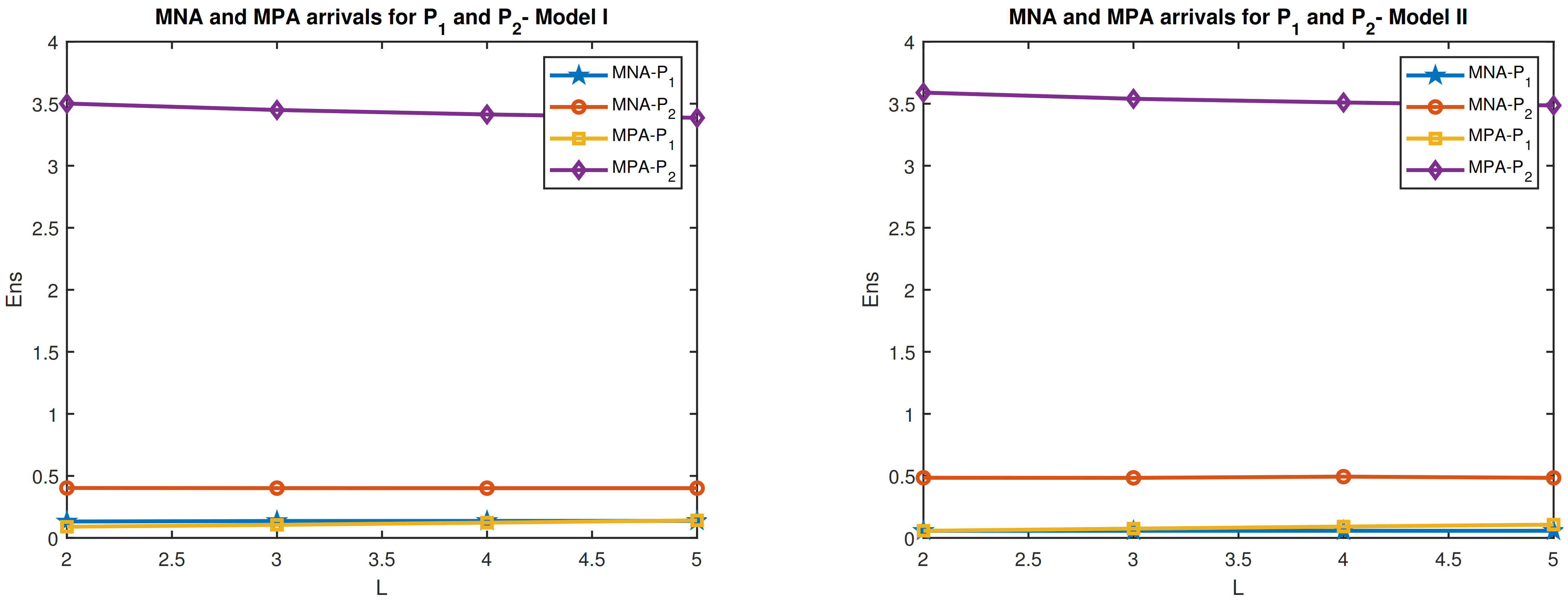
From Table 2, we can see that the expected number of $P_2$ customers increases as L increases in the case of EXP, HEXP, ERA (the rate of increase decreases as L increases), decreases in the case of MNA and MPA for both the models. This is due to the feedback effect and correlation effect in the case of MNA and MPA (also the arrival rate for all processes is fixed to a small value (0.1)). Furthermore, the expected number of $P_2$ customers in the case of preemptive service discipline is much more than that in the non-pre-emptive case (see Figure 1; the blue curve is invisible in the graph as there is not much difference in the expected number of $P_1$ customers in case of MPA and MNA). In the figures, Ens denotes the expected number of customers in the system and Ewt denote the expected waiting time of customers in the system.

From Table 3, we can see that as $\theta$ increases, the expected number of $P_1$ customers increases for all arrival processes in the case of model I and remains constant for different arrival processes in the case of model II. This is due to the feedback effect in the case of model I, but feedback does not affect $P_1$ customers in the case of model II.

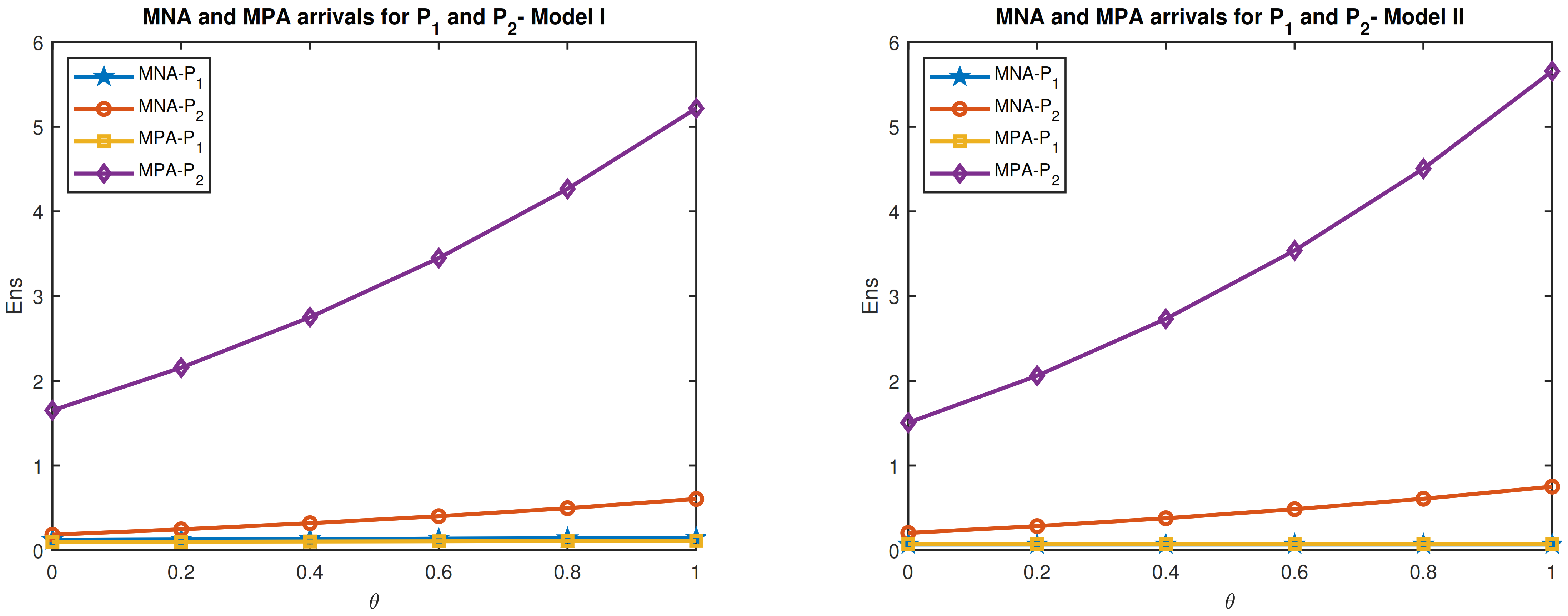
From Table 4, we can see that as $\theta$ increases, the expected number of $P_2$ customers increases for all arrival processes in the case of model I and model II. This is due to the feedback effect (see Figure 2. The blue curve is invisible in the graph as there is not much difference in the expected number of $P_1$ customers in the case of MPA and MNA).

From Table 2 and Table 4, we can see that the expected number of $P_2$ customers is much bigger for MPA. This is due to the correlation effect. From Table 1 and Table 3, we can see that the expected number of $P_1$ customers is lesser for model II compared to model I. Also, from Table 2 and Table 4, we can see that the expected number of $P_2$ customers is much bigger for model II compared to model I (in the case of MPA, the expected number becomes bigger when the feedback rate is high due to correlation effect).

10.2. Expected Waiting Time

Table 5. Effect of L on expected waiting time of $P_1$ customers in the system (when $\theta =0.6$).

L	Model I					Model II
	EXP	ERA	HEXP	MNA	MPA	EXP	ERA	HEXP	MNA	MPA
2	1.0712	1.0414	1.0493	1.0796	1.0907	0.9018	0.8989	0.9028	0.9114	0.9121
3	1.0766	1.0419	1.0543	1.0852	1.1001	0.9021	0.8989	0.9033	0.9124	0.9274
4	1.0775	1.0419	1.0553	1.0861	1.1150	0.9021	0.8989	0.9033	0.9125	0.9428
5	1.0776	1.0419	1.0555	1.0863	1.1317	0.9021	0.8989	0.9033	0.9125	0.9573

and

Table 6. Effect of L on expected waiting time of $P_2$ customers in the system (when $\theta =0.6$).

L	Model I					Model II
	EXP	ERA	HEXP	MNA	MPA	EXP	ERA	HEXP	MNA	MPA
2	3.6377	3.5569	3.6488	3.6766	9.2171	4.0102	3.7665	4.1070	4.7945	9.4702
3	3.6422	3.5567	3.6550	3.6740	8.7061	4.0118	3.7665	4.1097	4.7937	9.3680
4	3.6429	3.5567	3.6563	3.6733	8.4624	4.0119	3.7665	4.1099	4.7936	9.2446
5	3.6430	3.5567	3.6565	3.6732	8.3021	4.0119	3.7665	4.1099	4.7936	9.1352

show the effect of L on the expected waiting time of $P_1$ and $P_2$ customers in the system for model I(non-preemptive case) and model II (preemptive case) respectively.

Table 7. Effect of $\theta$ on expected waiting time of $P_1$ customers in the system (when $L=3$).

$\mathit{\theta }$	Model I					Model II
	EXP	ERA	HEXP	MNA	MPA	EXP	ERA	HEXP	MNA	MPA
0	0.9828	0.9579	0.9815	1.0069	1.0300	0.9021	0.8997	0.9031	0.9117	0.9252
0.2	1.0114	0.9842	1.0059	1.0304	1.0519	0.9021	0.8994	0.9031	0.9119	0.9259
0.4	1.0426	1.0121	1.0303	1.0564	1.0752	0.9021	0.8992	0.9032	0.9121	0.9266
0.6	1.0766	1.0419	1.0543	1.0852	1.1001	0.9021	0.8989	0.9033	0.9124	0.9274
0.8	1.1140	1.0738	1.0779	1.1172	1.1268	0.9021	0.8986	0.9034	0.9127	0.9283
1	1.1551	1.1082	1.1009	1.1529	1.1556	0.9021	0.8983	0.9035	0.9131	0.9293

and

Table 8. Effect of $\theta$ on expected waiting time of $P_2$ customers in the system (when $L=3$).

$\mathit{\theta }$	Model I					Model II
	EXP	ERA	HEXP	MNA	MPA	EXP	ERA	HEXP	MNA	MPA
0	3.5018	3.4623	3.5047	3.5223	6.3444	3.8240	3.9046	3.6427	4.6121	6.7614
0.2	3.5413	3.4912	3.5461	3.5626	7.0025	3.8738	3.9579	3.6784	4.6594	7.4534
0.4	3.5874	3.5225	3.5954	3.6124	7.7768	3.9354	4.0250	3.7193	4.7190	8.3122
0.6	3.6422	3.5567	3.6550	3.6740	8.7061	4.0118	4.1097	3.7665	4.7937	9.3680
0.8	3.7081	3.5946	3.7283	3.7505	9.8063	4.1073	4.2172	3.8212	4.8878	10.6518
1	3.7885	3.6368	3.8196	3.8458	11.1251	4.2273	4.3543	3.8850	5.0066	12.2415

show the effect of $\theta$ on the the expected waiting time of $P_1$ and $P_2$ customers in the system respectively in both models.

From Table 5, we can see that the expected waiting time increases as L increases for all arrival processes in both models. This happens since when L increases, the expected number of $P_1$ customers increases, and hence the expected number of feedback customers also increases. As expected, the expected waiting time of $P_1$ customers in the case of pre-emptive service discipline is less than that in the non-pre-emptive case.

From Table 6, we can see that the expected waiting time decreases as L increases for all arrival processes except in the cases of EXP and HEXP in model I. This is because when L increases, the expected number of $P_1$ customers increases in the cases of EXP, ERA, and HEXP and decreases in the case of MNA and MPA due to the correlation effect. However, the rate of increase in the case of ERA is very small. This all happens as we fixed our arrival rate to a small quantity (0.1). However, both, the rate of increase and the rate of decrease, decrease as L increases. This happens as when L increases, the expected number of $P_1$ customers increases, and when it hits L, the effect of L decreases. As a result, the expected number of feedback customers increases in the case of EXP and HEXP and decreases in all other cases. Hence, the expected waiting time decreases for all arrival processes except in the cases of EXP and HEXP as L increases.

Again, from Table 6, in the case of model II, the expected waiting time of $P_2$ customers is more than that in model I, as we expected. In this case, the expected waiting time increases in the cases of EXP and HEXP, decreases and then stays constant in the case of ERA and decreases in the cases of MNA and MPA as L increases. This is because when L increases, the expected number of $P_1$ customers increases in the cases of EXP and HEXP, stays constant in the case of ERA and decreases in the case of MNA and MPA (due to the correlation effect). This all happens as we fixed our arrival rate to a small quantity (0.1). As expected, the expected waiting time of $P_2$ customers in the case of preemptive service discipline is more than that in the non-preemptive case. (see Figure 3. The blue curve is invisible in the graph as there is not much difference in the expected waiting time of $P_1$ customers in the case of MPA and MNA).

Next, we fixed $L=3$. From Table 7, we can see that the expected waiting time of $P_1$ customers increases as $\theta$ increases for all arrival processes in model I. This happens since when $\theta$ increases, the expected number of feedback customers increases, and the expected number of customers in the $P_2$ queue increase. As the service discipline is non-pre-emptive, this will also affect $P_1$ customers. Hence, the expected waiting time of $P_1$ customers increases as $\theta$ increases for all arrival processes.

Again, from Table 7, we can see that the expected waiting time decreases as $\theta$ increases for all arrival processes in model II. This happens since when $\theta$ increases, the expected number of feedback customers increases, and the expected number of customers in the $P_2$ queue increases. However, as the service discipline is preemptive, this will not have much effect on $P_1$ customers.

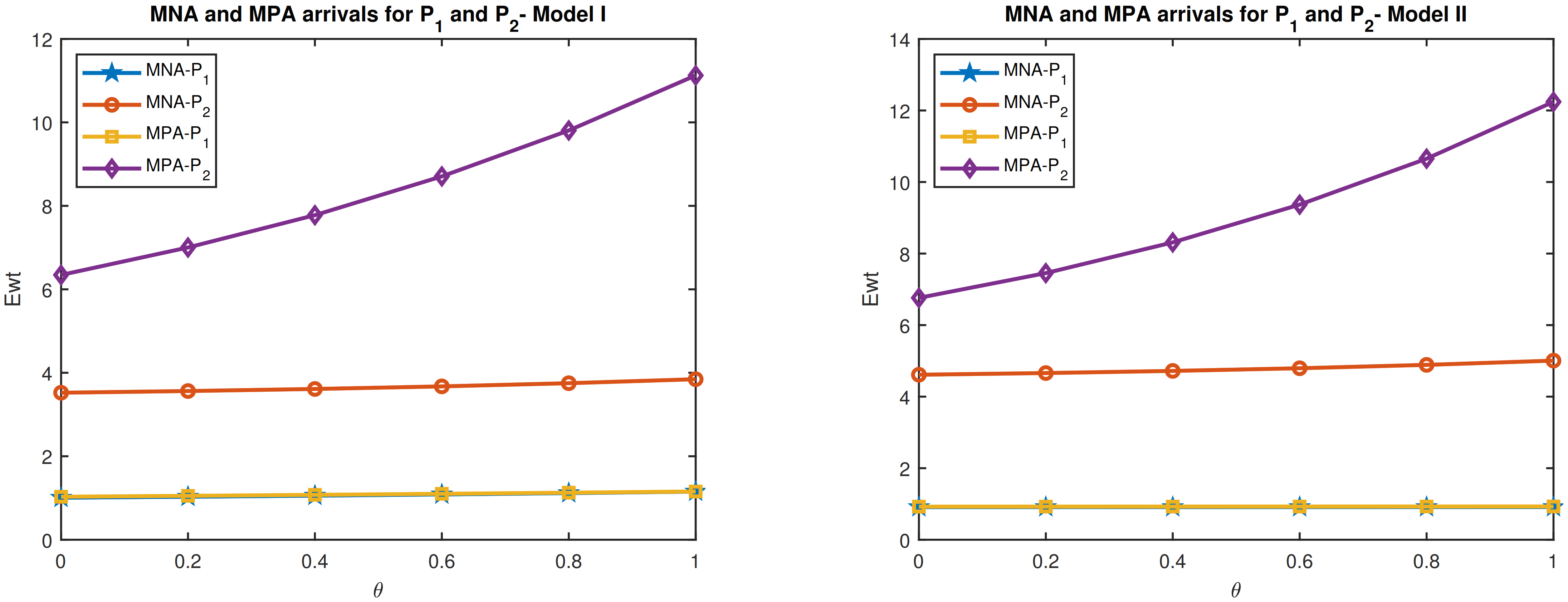
From Table 8, we can see that the expected waiting time of $P_2$ customers increases as $\theta$ increases for all arrival processes in both model I and model II. This happens since when $\theta$ increases, the expected number of feedback customers increases, and the expected number of customers in the $P_2$ queue increases. (see Figure 4. The blue curve is invisible in the graph as there is not much difference in the expected waiting time of $P_1$ customers in the case of MPA and MNA).

We can see that, in both the models, among all arrival processes, the expected waiting time is longer in the case of MPA. This is due to the correlation effect.

11. Conclusions

In this paper, we analyzed two single server queueing models with priority customers. High priority customers were allowed exactly one feedback if they wished so. However, feedback results in the loss of their priority status. The inflow of customers forms an MMAP and service of the distinct class of customers are according to two independent, non-identical phase-type distributions. The stationary distributions of both systems are derived and expressions for several performance characteristics are obtained. The numerical illustrations provided throw light on the relative performance of the two models.

One possible extension of this work is to examine the case of infinite capacity waiting stations for all classes of priority. This can be approached through the method of roots as discussed in papers by Chaudhry et al. [42]. It is also interesting to compare two different situations: in one, the external customers join only in the highest priority line, and in the second, low priority customers join in the respective queues.

References

1. Krishnamoorthy, A.; Manjunath, A.S. On Queues with Priority Determined by Feedback. Calcutta Stat. Assoc. Bull. 2018, 70, 33–56. [Google Scholar] [CrossRef]
2. Takacs, L. A single-server queue with feedback. Bell Syst. Tech. J. 1963, 42, 509–519. [Google Scholar] [CrossRef]
3. Takacs, L. A queuing model with feedback. Oper. Res. 1977, 11, 345–354. [Google Scholar] [CrossRef]
4. Koroliuk, V.S.; Melikov, A.Z.; Ponomarenko, L.A.; Rustamov, A.M. Methods for analysis of multi-channel queueing models with instantaneous and delayed feedbacks. Cybern. Syst. Anal. 2016, 52, 58–70. [Google Scholar] [CrossRef]
5. Melikov, A.Z.; Ponomarenko, L.A.; Rustamov, A.M. Methods for analysis of queuing models with instantaneous and delayed feedbacks. Commun. Comput. Inf. Sci. 2015, 564, 185–199. [Google Scholar]
6. Rajadurai, P.; Saravanarajan, M.C.; Chandrasekaran, V.M. A study on M/G/1 feedback retrial queue subject to server breakdown and repair under multiple working vacation policy. Alex. Eng. J. 2018, 57, 947–962. [Google Scholar] [CrossRef]
7. Ke, J.C.; Liu, T.H.; Su, S.; Zhang, Z.G. On retrial queue with customer balking and feedback subject to server breakdowns. Commun. Stat. Theory Methods 2020. [Google Scholar] [CrossRef]
8. Singh, C.J.; Kaur, S.; Jain, M. Waiting time of bulk arrival unreliable queue with balking and Bernoulli feedback using maximum entropy principle. J. Stat. Theory Pract. 2017, 11, 41–62. [Google Scholar] [CrossRef]
9. Jailaxmi, V.; Arumuganathan, R.; Rathinasamy, A. Performance analysis of an M[X]/G/1 feedback retrial queue with non-persistent customers and multiple vacations with N-policy. Int. J. Oper. Res. 2017, 29, 149–169. [Google Scholar] [CrossRef]
10. Chang, C.J.; Ke, J.C.; Chang, F.M. Unreliable retrial queue with loss and feedback under threshold-based policy. Int. J. Ind. Syst. Eng. 2018, 30, 1–20. [Google Scholar] [CrossRef]
11. Chang, F.M.; Liu, T.H.; Ke, J.C. On an unreliable-server retrial queue with customer feedback and impatience. Appl. Math. Model. 2018, 55, 171–182. [Google Scholar] [CrossRef]
12. Madheswari, P.; Krishna Kumar, B.; Suganthi, P. Analysis of M/G/1 retrial queues with second optional service and customer balking under two types of Bernoulli vacation schedule. RAIRO Oper. Res. 2019, 53, 415–443. [Google Scholar] [CrossRef]
13. Melikov, A.; Aliyeva, S.; Sztrik, J. Analysis of Instantaneous Feedback Queue with Heterogeneous Servers. Mathematics 2020, 8, 2186. [Google Scholar] [CrossRef]
14. Jain, M.; Kaur, S. Bernoulli vacation model for M[X]/G/1 unreliable server retrial queue with Bernoulli feedback, balking and optional service. RAIRO-Oper. Res. 2021, 55, 2027. [Google Scholar] [CrossRef]
15. Vijaya Laxmi, P.; Girija Bhavani, E.; Kumar, R. Correlated reneging in an optional service Markovian queue with working vacations. Reliab. Theory Appl. 2020, 15, 102–116. [Google Scholar]
16. Bouchentouf, A.A.; Cherfaou, M.; Boualem, M. Performance and economic analysis of a single server feedback queueing model with vacation and impatient customers. OPSEARCH 2019, 56, 300–323. [Google Scholar] [CrossRef]
17. Zhao, Y.; Yue, W. Performance analysis and optimization for cognitive radio networks with a finite primary user buffer and a probability returning scheme. J. Ind. Manag. Optim. 2020, 16, 1119–1134. [Google Scholar] [CrossRef]
18. Melikov, A.Z.; Aliyeva, S.H.; Shahmaliyev, M.O. Methods for Computing a System with Instantaneous Feedback and Variable Input Stream Intensity. Autom. Remote Control 2020, 81, 1647–1658. [Google Scholar] [CrossRef]
19. Melikov, A.Z.; Aliyeva, S.; Sztrik, J. Analysis of queuing system MMPP/M/K/K with delayed feedback. Mathematics 2019, 7, 1128. [Google Scholar] [CrossRef] [Green Version]
20. White, H.; Christie, L.S. Queueing with Preemptive Priorities or with Breakdown. Oper. Res. 1958, 6, 79–96. [Google Scholar] [CrossRef]
21. Jaiswal, N.K. Preemptive resume priority queue. Oper. Res. 1961, 9, 732–742. [Google Scholar] [CrossRef]
22. Jaiswal, N.K. Time dependent solution of the head of the line priority queue. J. R. Stat. Soc. B. 1962, 24, 73–90. [Google Scholar] [CrossRef]
23. Cobham, A. Priority Assignment in Waiting Line Problems. Oper. Res. 1954, 2, 70–76. [Google Scholar] [CrossRef]
24. Jaiswal, N.K. Priority Queues; Academic Press: New York, NY, USA; London, UK, 1968. [Google Scholar]
25. Takagi, H. Queueing Analysis, Volume I: Vacation and Priority Systems, Part 1; Elsevier: Amsterdam, The Netherlands, 1991. [Google Scholar]
26. Brodal, G.S. A survey on Priority Queues: Volume 8066 of the series Lecture Notes in Computer Science; Springer: Berlin, Germany, 2013; pp. 150–163. [Google Scholar]
27. Krishnamoorthy, A.; Pramod, P.K.; Chakravarthy, S.R. Queues with interruptions: A survey. TOP 2014, 22, 290–320. [Google Scholar] [CrossRef]
28. Jacob, V.; Chakravarthy, S.R.; Krishnamoorthy, A. On a Customer Induced Interruption in a service system. Stoch. Anal. Appl. 2012, 30, 949–962. [Google Scholar] [CrossRef]
29. Krishnamoorthy, A.; Jacob, V. Analysis of Customer Induced Interruption in a multi server system. Neural Parallel Sci. Comput. 2012, 20, 153–172. [Google Scholar]
30. Dudin, A.N.; Jacob, V.; Krishnamoorthy, A. A multi-server queueing system with service interruption, partial protection and repetition of service. Ann. Oper. Res. 2015, 233, 101–121. [Google Scholar] [CrossRef]
31. Manjnath, A.S. Analysis Of Some Priority Queues and a Problem on Diagonostics. Ph.D. Thesis, Cochin University of Science & Technology, Kochi, India, 2017. [Google Scholar]
32. Boxma, O.J.; Yechiali, U. An M/G/1 queue with multiple types of feedback and gated vacations. J. Appl. Probab. 1997, 34, 773–784. [Google Scholar] [CrossRef]
33. Choi, B.D.; Kim, B. M/G/1 queueing system with fixed feedback policy. ANZIAM J. 2002, 44, 283–297. [Google Scholar] [CrossRef] [Green Version]
34. Choi, B.D.; Kim, B.; Choi, S.H. An M/G/1 queue with multiple types of feedback, gated vacations and FCFS policy. Comput. Oper. 2003, 30, 1289–1309. [Google Scholar] [CrossRef]
35. Choi, B.D.; Kulkarni, V.G. Feedback Retrial Queueing Systems. Queueing and Related Models; Bhat, U.N., Basawa, I.V., Eds.; Oxford University Press: New York, NY, USA, 1992; pp. 93–105. [Google Scholar]
36. Jewkes, E.M.; Buzacott, J.A. Flow time distributions in a K class M/G/1 priority feedback queue. Queueing Syst. 1991, 8, 183–202. [Google Scholar] [CrossRef]
37. Simon, B. Priority queues with feedback. J. Assoc. Comput. Mach. 1984, 31, 134–149. [Google Scholar] [CrossRef]
38. Krishna Kumar, B.; Pavai Madheswari, S.; Vijayakumar, A. The M/G/1 retrial queue with feedback and starting failures. Appl. Math. Model. 2002, 26, 1057–1075. [Google Scholar] [CrossRef]
39. Krishna Kumar, B.; Rukmani, R.; Thangaraj, V. On multi server. feedback retrial queue with finite buffer. Appl. Math. Model. 2009, 33, 2062–2083. [Google Scholar] [CrossRef]
40. Kumar, B.K.; Vijayalakshmi, G.; Krishnamoorthy, A.; Basha, S.S. A single server feed back retrial queue with collisions. Comput. Oper. Res. 2010, 37, 1247–1255. [Google Scholar] [CrossRef]
41. Neuts, M.F. Matrix Geometric Solutions in Stochastic Models: An Algorithmic Approach; The Johns Hopkins University Press: Baltimore, MD, USA, 1981. [Google Scholar]
42. Chaudhry, M.L.; Kim, J.J.; Banik, A.D. Analytically Simple and Computationally Efficient Results for the GIX/Geo/c Queues. J. Probab. Stat. 2019, 2019, 6480139. [Google Scholar] [CrossRef] [Green Version]
Figure 1. Effect of L on expected number of P 1 and P 2 customers in the system for MNA and MPA arrival processes with correlation of −0.4211 and 0.4211, respectively(when θ = 0.6 ).
Mathematics 09 01797 g001
Figure 2. Effect of θ on expected number of P 1 and P 2 customers in the system for MNA and MPA arrival processes with correlation of −0.4211 and 0.4211, respectively (when L = 3 ).
Mathematics 09 01797 g002
Figure 3. Effect of L on expected waiting time of P 1 and P 2 customers in the system for MNA and MPA arrival processes with correlation of −0.4211 and 0.4211, respectively (when θ = 0.6 ).
Mathematics 09 01797 g003
Figure 4. Effect of θ on expected waiting time of P 1 and P 2 customers in the system for MNA and MPA arrival processes with correlation of −0.4211 and 0.4211, respectively (when L = 3 ).
Mathematics 09 01797 g004