Article

On Machine-Learning Morphological Image Operators

by
Nina S. T. Hirata
1,* and
George A. Papakostas
2,*
1
Department of Computer Science, Institute of Mathematics and Statistics, University of São Paulo, São Paulo 05508-090, Brazil
2
HUMAIN-Lab, Department of Computer Science, International Hellenic University, 65404 Kavala, Greece
*
Authors to whom correspondence should be addressed.
Mathematics 2021, 9(16), 1854; https://doi.org/10.3390/math9161854
Submission received: 14 June 2021 / Revised: 18 July 2021 / Accepted: 29 July 2021 / Published: 5 August 2021

Abstract

:
Morphological operators are nonlinear transformations commonly used in image processing. Their theoretical foundation is based on lattice theory, and it is a well-known result that a large class of image operators can be expressed in terms of two basic ones, the erosions and the dilations. In practice, useful operators can be built by combining these two operators, and the new operators can be further combined to implement more complex transformations. The possibility of implementing a compact combination that performs a complex transformation of images is particularly appealing in resource-constrained hardware scenarios. However, finding a proper combination may require a considerable trial-and-error effort. This difficulty has motivated the development of machine-learning-based approaches for designing morphological image operators. In this work, we present an overview of this topic, divided in three parts. First, we review and discuss the representation structure of morphological image operators. Then we address the problem of learning morphological image operators from data, and how representation manifests in the formulation of this problem as well as in the learned operators. In the last part we focus on recent morphological image operator learning methods that take advantage of deep-learning frameworks. We close with discussions and a list of prospective future research directions.

1. Introduction

Images are a rich source of information. To extract useful information, images are usually carefully processed to highlight or segment objects or other information of interest. In the context of cyber-physical systems (CPS) [1,2], the ability to efficiently process image data and act according to the extracted information would enable the development of many useful applications. However, running complex and heavy computing code such as those required in typical image analysis in hardware constrained devices is still a challenge. To cope with processing limitations of these devices, a traditional approach is to rely on centralized data centers with processing servers, such as cloud computing platforms, for data processing. This arrangement enables devices to relocate most of the heavy processing to these centers. However, latency is a critical drawback, especially when large amounts of data need to be transmitted back and forth between the devices and these processing centers. Due to this drawback, the concept of edge computing, i.e., bringing data and computation closer to where they are needed, is gaining increasing attention [3]. Edge computing pushes to the surface the need for boosting computing capabilities and intelligent processing in hardware constrained devices [4]. Obviously, these limitations can be mitigated by improving processing capabilities on the hardware side, but at the same time improvements can be sought on the software side, by developing well designed and customized algorithms that take advantage of specific characteristics of the hardware as well as are efficient in terms of memory usage and processing.
Theoretical models for image processing algorithms are divided into linear and nonlinear approaches. Both offer a range of techniques and tools for building image processing pipelines. Although linear models are well studied and understood, there are a few theories for modeling nonlinear transformations [5]. Mathematical morphology is one of the nonlinear models and its fundamentals are based on lattice theory [6,7].
In general, the complexity of building image processing pipelines has motivated the use of machine-learning techniques. Recent developments in machine-learning and deep-learning techniques brought huge advances in Image Processing and Computer Vision. The core processing units in a Convolutional Neural Network (CNN)—the basic deep neural network model used in image processing—are linear functions, popularly called convolutions, followed by nonlinear activations [8]. These networks are trained end-to-end for a diversity of Computer Vision tasks such as image classification, image segmentation, object detection, and scene description, and convolution kernel weights are learned from data. One of the characteristics that explains the success of deep-learning algorithms is their ability to learn discriminative representation of data, in a data-driven fashion, enabling easier adaptation of the algorithms for each use-case scenario. Current state of the art methods in image processing to perform image-to-image transformations such as the ones shown in Figure 1 are based on fully convolutional neural networks [9,10]. These networks have many parameters and are usually run on GPU for efficient processing. Compressing deep network models is also an active research field [11,12,13].
In morphological image processing, one can build pipelines that perform complex image transformations by composing two basic operators, erosions and dilations, and others built from them [6,19,20]. Some degree of success has been achieved by machine-learning-based design methods, in restricted situations such as in binary image processing [21,22], in learning subfamilies of operators [23], or in specific applications [24]. However, designing optimal processing pipelines consisting of sequential composition of operators is an unsolved problem, as they usually lead to large combinatorial problems. More recently, deep morphological neural networks (DMNN), built by replacing the standard “linear convolution+nonlinear activation” layers of deep neural networks with erosion or dilation layers, started to emerge [25,26,27,28]. This is enabling the optimization of sequential compositions of morphological operators. Among other potential benefits associated with DMNNs, interpretability (morphological operators provide insights as they probe geometrical and topological information) and reduced size (morphological operators are nonlinear and thus more expressive) are often cited. The latter is particularly appealing to CPS applications.
The aim of this paper is to gather information about morphological image operator learning regarding image transformations much like the ones shown in Figure 1, and present a comprehensive panorama of the subject. In Section 2, mathematical morphology is revisited, with focus on representation related issues, and pointers to relevant literature. We review basic concepts and properties of morphological image operators, initially restricted to binary images to highlight common structural constructs between them and logical functions. We also briefly recall the extension of the same concepts and properties to gray-level images and the connections to lattice computing. In Section 3, we first characterize the problem of learning morphological operators from training data, and then we examine some existing learning methods, with particular interest in aspects related to underlying morphological representation and connections to machine-learning techniques. Then, in Section 4 we survey recently proposed image processing deep morphological networks, where the elementary morphological operators and their parameters are optimized using the standard gradient descent backpropagation algorithm. In Section 5 and Section 6 we present some discussions, directions for future research, and conclusions.

2. Morphological Representations

Morphological operators were first developed for binary images, based on a set theoretic formulation [6,29]. Later it has been extended for gray-level images, and then their lattice-theoretical foundation has been established [7,30]. From a strict mathematical point of view, Mathematical Morphology is concerned with lattice operators. The relevant point to be noted here is that images and several other types of signals can be modeled as lattice elements. Thus, image transformations can be formally modeled and examined using the tools provided by Mathematical Morphology. The characterization of the lattice of images and the lattice of image operators are extensively reported in the literature [7,31,32]. In this section, we recall some results related to image operator representation, restricting the scope to discrete images. We start with a focus on binary morphology, defining erosion and dilation, their role in the decomposition structure of translation-invariant operators, and highlighting the connections with logical functions. At the end of the section, we comment on the extension of these representations to grayscale images.

2.1. Binary Image Processing

Let E = Z 2 be the image domain, and let o denote its origin. A binary image on E is a function I : E { 0 , 1 } , and it can be seen as the characteristic (indicator) function of a set. Conversely, any set S E can be represented by its indicator function. Thus, both { 0 , 1 } E and P ( E ) (the power set of E) can be used to denote the set of all binary images defined on E. For convenience, we will use the same symbol for the function and set notation of an image, i.e., given a binary image I, we write interchangeably I ( p ) = 1 or p I to indicate that p is a foreground pixel of I. Given a set S P ( E ) , S c is the complement of S, S ˇ = { p : p S } is the reflection of S, and S q = { p + q : p S } is the translation of S by vector q.
Let I be a binary image, and B a structuring element (usually a small set located at the origin of E). Erosion ( ε B ( I ) ) and dilation ( δ B ( I ) ) are the two building block operators used to define many other operators, and are defined as:
ε B ( I ) = { p E : B p I }
δ B ( I ) = { p E : B ˇ p I }
A third basic operator is the hit-or-miss (HMT), characterized by a pair ( A , B ) of structuring elements such that A B = , defined as:
H ( A , B ) ( I ) = { p E : A p I } { p E : B p I c } = ε A ( I ) ε B ( I c ) .
Related to this, there is the interval (also, wedge [7]) operator parameterized by an interval [ A , B ] = { X : A X B } , with A B , defined as:
Λ ( A , B ) ( I ) = { p E : A p I B p }
It can be shown that Λ ( A , B ) = H ( A , B c ) [7]. They are related to template matching.
For these operators, the output value of the transformed image at a given point p does not depend on p; it depends only on the image values on a finite support region W p around p ( W = B for ε B , W = B ˇ for δ B , and W = ( A B ) for the hit-or-miss operators). By cascading erosions and dilations, as well as composing them by means of set operations (union, intersection and complementation), new operators can be built [19,20]. In these composed operators, the invariance with respect to location p is preserved, although with possibly larger support region W. For example, Figure 2 illustrates the support region of an opening ( γ B ( I ) = δ B ( ε B ( I ) ) ) on the 1-D domain.

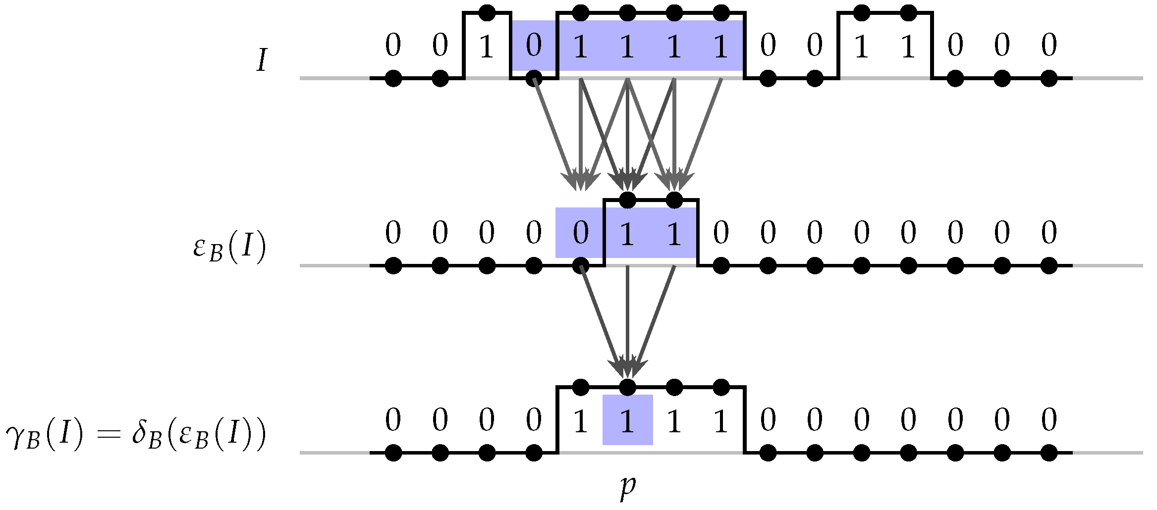
2.1.1. Translation Invariance and Local Definition

If only finite structuring elements and only a finite number of operators are used in the composition, the support region W is of finite size. Therefore, these operators are locally defined, meaning that [ Ψ ( I ) ] ( p ) = 1 [ Ψ ( I W z ) ] ( p ) = 1 for any W W . Moreover, since they are invariant with respect to p, these operators are translation-invariant, meaning that [ Ψ ( I ) ] p = Ψ ( I p ) , I P ( E ) , p E . In particular, translation-invariance implies that p can be dropped and the operator can be characterized in terms of its behavior at the origin. More specifically, translation-invariant operators can be described in terms of their kernel and bi-kernel [7,33]. The kernel of Ψ : P ( E ) P ( E ) is defined as K ( Ψ ) = { I P ( E ) : o Ψ ( I ) } and the bi-kernel is defined as K ( Ψ ) = { ( A , B ) P ( E ) × P ( E ) : A B , [ A , B ] K ( Ψ ) } . Two important decomposition results are the following.
Theorem 1
([34]). Let Ψ be a translation-invariant increasing set operator (i.e., X Y Ψ ( X ) Ψ ( Y ) ). Then
Ψ ( I ) = A K ( Ψ ) ε A ( I )
Theorem 2
([33]). Let Ψ be a translation-invariant set operator. Then
Ψ ( I ) = ( A , B ) K ( Ψ ) Λ ( A , B ) ( I )
These two theorems state that a translation-invariant set operator can be characterized in terms of its kernel elements. See a proof in [7]. The first is actually a particular case of the second, since for increasing operators it holds that B = E and thus the interval operator can be characterized in terms of its lower extreme only. Later, a compact representation was proposed initially for increasing operators [31], and then extended for non-necessarily increasing operators [33], in terms of the basis of an operator defined as B ( Ψ ) = { [ A , B ] P ( E ) : [ A , B ] is a maximal interval contained in K ( Ψ ) } . In terms of its basis, a translation-invariant operator can be expressed as
Ψ ( I ) = [ A , B ] B ( Ψ ) Λ ( A , B ) ( I ) .
Another important result, as a consequence of translation invariance and local definition properties, is the characterization of these operators in terms of a local function. More specifically, any binary image operator Ψ : P ( E ) P ( E ) satisfying translation invariance and local definition with respect to W can be uniquely characterized by a local function ψ : P ( W ) { 0 , 1 } , as follows [7]:
p Ψ ( I ) ψ ( I p W ) = 1 .
The argument I p W of function ψ is an element of P ( W ) , the set of all binary images defined on W. The local functions are precisely the set of Boolean (logic) functions on n = | W | (cardinality of W) variables [7], as detailed next.

2.1.2. Connection with Boolean Functions

The correspondence between image operators and logic functions can be established as follows. Let us suppose that W = { w 1 , w 2 , , w n } and let us assign a binary variable x i for w i , i = 1 , , n . Then, for any image I and position p E , to compute the value ψ ( x 1 , x 2 , , x n ) of a logic function, we set x i = 1 w i + p W p I (or, equivalently, I ( w i + p ) = 1 ). For instance, the logic function ψ ε that characterizes an erosion is one that outputs 1 only when B p I , i.e., when B p I = B p . Thus, if we set W = B , this means ψ ε outputs 1 only when x 1 = x 2 = = x n = 1 . Thus, ψ ε ( x 1 , , x n ) = x 1 x 2 x n . For the dilation to output 1, one point in B ˇ p I is sufficient. Thus, the logic function that characterizes the dilation is ψ δ ( x 1 , , x n ) = x 1 + x 2 + + x n . For the hit-or-miss, we have a logic product where variables assigned to A appear uncomplemented ( x i , meaning that it hits the foreground) and those assigned to B appear complemented ( x ¯ i , meaning that it hits the background and therefore it misses the foreground). Please note that there is no harm if we consider a larger support W , W W , for operators that are locally defined with respect to W, since it is always possible to define a logic function on | W | variables in such a way that those variables assigned to points in W \ W will have no relevance in the logic function computation.

2.1.3. The Lattice of Translation-Invariant and Locally Defined Binary Image Operators

Besides the characterization by a local function (Equation (8)), an important consequence of translation invariance and local definition properties is the fact that the kernel and the basis as defined before can be restricted to the finite domain W: the kernel becomes K ( Ψ ) = { I P ( W ) : ψ ( I ) = 1 } and the basis is formed by all maximal intervals contained in K ( Ψ ) .
The set P ( W ) with the usual set inclusion ⊆ is a Boolean lattice. The set { 0 , 1 } n equipped with the partial order relation ≤ defined as, for any x , y { 0 , 1 } n , x y x i y i , i = 1 , , n , and the operations x + y , x · y , x ¯ , point-wise extension of the binary logic operations +, ·, and ¯ , is also a Boolean lattice. It is well known that any non-null element in { 0 , 1 } n can be expressed uniquely as a join (component-wise logical sum) of a subset of the atomic elements ( 1 , 0 , , 0 , 0 ) , ( 0 , 1 , , 0 , 0 ) , , ( 0 , 0 , , 1 , 0 ) , ( 0 , 0 , , 0 , 1 ) , just like any set can be expressed as a union of unitary sets corresponding to each of its elements. The set of all Boolean functions of the form f : { 0 , 1 } n { 0 , 1 } with operations and partial order relation inherited from ( { 0 , 1 } , ) is also a complete lattice, isomorphic to the lattice ( P ( P ( W ) ) , ) .
Figure 3 shows the lattice of all Boolean functions on two variables, x 1 and x 2 . Please note that the atomic functions are x ¯ 1 x ¯ 2 , x ¯ 1 x 2 , x 1 x ¯ 2 and x 1 x 2 . Any non-null Boolean function on 2 variables can be written as a sum of these atomic functions. Moreover, supposing W = { w 1 , w 2 } , we have P ( W ) = { { } , { w 1 } , { w 2 } , { w 1 , w 2 } } , which is equivalent to { 0 , 1 } 2 = { 00 , 10 , 01 , 11 } . Function f 3 ( x 1 , x 2 ) = x ¯ 1 x ¯ 2 + x ¯ 1 x 2 = x ¯ 1 , corresponds to the operator with kernel { 00 , 01 } , which corresponds to the basis consisting of only one interval, [ 00 , 01 ] (or, equivalently, [ , { w 2 } ] ).

2.1.4. Representation Structures

As discussed above, there is a one-to-one relation between the elements in K ( Ψ ) and the product terms in the canonical sum-of-products form of the logic function that characterizes Ψ . Moreover, the intervals in B ( Ψ ) correspond to the irreducible product terms of the logic expression, when it is expressed in a minimal sum-of-products form. We note that Boolean functions can be expressed in canonical sum-of-products as well as in canonical product-of-sums forms. Similarly, image operators can be expressed as union of intervals operators or as intersection of dual interval operators. However, in this paper we consider only the sum-of-products form. See more details, for instance, in [33].
Before proceeding, we examine another example that illustrates the relation between image operators and its corresponding characteristic logic function. The median filter is a sliding window operator that, for each pixel p, computes the median value of the set of values of an image I under W p . If we suppose W = { w 1 , w 2 , w 3 } and x 1 , x 2 , x 3 the corresponding binary variables, the logic function that characterizes the median filter is given by f ( x 1 , x 2 , x 3 ) = x 1 x 2 + x 1 x 3 + x 2 x 3 . It is easy to see that this function will output 1 only if at least two of the three observed values are equal to 1, agreeing with the definition of median value. Median filters are increasing operators, and thus they can be expressed as a union of erosions. As it can be seen, the Boolean function is positive and each of the product terms corresponds to an erosion.
In the field of Boolean functions, this representation as a sum of products is formally well characterized [35]. On the other hand, as we have already discussed, image operators can be expressed as a sequential composition of simpler operators. Thus, it is interesting to have a look into sequential compositions of Boolean functions. Let us take the previously discussed opening γ B ( I ) = δ B ( ε b ( I ) ) as an example. The standard way to compute openings is to first compute I = ε B ( I ) and then γ B ( I ) = δ B ( I ) . This means that first ψ ε is applied pixel-by-pixel on I and then ψ δ is applied, also pixel-by-pixel, on I . As discussed above, supposing B consists of n points, we have ψ ε ( x 1 , , x n ) = x 1 x 2 x n and ψ δ ( x 1 , , x n ) = x 1 + x 2 + + x n . The logic function that characterizes the opening operator can be calculated as the composition of these two logic functions. For instance, letting B = { 1 , 0 , 1 } , the opening γ B will correspond to a logic function ψ γ on 5 variables (see also Figure 2):
ψ γ ( x 1 , x 2 , x 3 , x 4 , x 5 ) = ψ δ ( ψ ε ( x 1 , x 2 , x 3 ) , ψ ε ( x 2 , x 3 , x 4 ) , ψ ε ( x 3 , x 4 , x 5 ) ) = x 1 x 2 x 3 + x 2 x 3 x 4 + x 3 x 4 x 5
Each of the variables is assigned to the respective point in the support region of the opening operator.
Equation (9) means that the opening can be computed by applying ψ γ pixel-by-pixel on I. Roughly speaking, we may say that the first definition ( γ B ( I ) = δ B ( ε b ( I ) ) ) is a sequential (deep) representation while the second one (Equation (9)) is a parallel (shallow) representation. For this example, there is exactly 2 5 possible images defined on W. Among them, the opening outputs value 1 for eight images, as shown in Figure 4. A Boolean function, on five variables in its canonical sum-of-products form, which outputs 1 for these, and only for these input, can be written straightforwardly as f ( x 1 , x 2 , x 3 , x 4 , x 5 ) = x ¯ 1 x ¯ 2 x 3 x 4 x 5 + x ¯ 1 x 2 x 3 x 4 x ¯ 5 + x 1 x 2 x 3 x ¯ 4 x ¯ 5 + x ¯ 1 x 2 x 3 x 4 x 5 + x 1 x ¯ 2 x 3 x 4 x 5 + x 1 x 2 x 3 x ¯ 4 x 5 + x 1 x 2 x 3 x 4 x ¯ 5 + x 1 x 2 x 3 x 4 x 5 . This corresponds to the kernel representation of the opening. This logic function can be reduced to f γ ( x 1 , x 2 , x 3 , x 4 , x 5 ) = x 1 x 2 x 3 + x 2 x 3 x 4 + x 3 x 4 x 5 as shown before (Equation (9)), and this reduced form corresponds to the minimal basis decomposition. Again, we have a positive function, meaning that the corresponding image operator is increasing, which is the case of openings.

2.2. Grayscale Image Processing

Grayscale images are functions of the form f : E K , where K = { 0 , 1 , , k 1 } is the set of grayscales. Binary images are just a particular case with k = 2 . In the same way the set inclusion ⊆ is a partial order relation, the relation ≤ defined as f g f ( p ) g ( p ) , p E , is also a partial order relation. To model grayscale images as lattice elements, a common approach is to consider an extended set R ¯ = R { , + } , which is a complete lattice, and consider images as functions from E to R ¯ , which inherits the lattice structure of R ¯ . For the case of a finite set of grayscales, we may consider the set K { , + } , and then formulas involving and + should be defined accordingly (see for instance [31,32] for more details). The translation of an image f by vector q is denoted f q and defined as f q ( p ) = f ( p q ) , p E . The vertical shift of an image f by a constant d is denoted f + d , and defined as ( f + d ) ( p ) = f ( p ) + d , p E .
The erosion and dilation of an image f by structuring function b : B K are defined respectively as:
[ ε b ( f ) ] ( p ) = m i n { f ( p + q ) b ( q ) : q B }
[ δ b ( f ) ] ( p ) = m a x { f ( p q ) + b ( q ) : q B }
Please note that b is a function with support B, thus sometimes it is called non-flat structuring element. Grayscale erosions and dilations are also commonly defined for flat structuring elements. A structuring function corresponding to a flat structuring element B can be expressed by setting b ( p ) = if p B , 0 if p B .
Thus, erosions and dilations with a flat structuring element B reduce respectively to:
[ ε B ( f ) ] ( p ) = m i n { f ( p + q ) : q B }
[ δ B ( f ) ] ( p ) = m a x { f ( p q ) : q B }
There are different definitions for grayscale HMT operators [36]. The underlying idea is similar to the template-matching behavior of binary HMT. In the grayscale case two structuring functions, one that fits the image from below and another that fits from above, are considered. One way to unify the different models is to think them as consisting of a fitting and a valuation steps, where fitting defines when a signal fits the pair of structuring functions and the valuation defines which value is output when fitting occurs [36].
In an analogous way as in the binary case, erosions, dilations and their compositions are translation-invariant and locally defined with respect to a support region W. Thus, they are also characterized by a local function ψ : K W K , where K W denotes all images with values in K, defined on a support region W:
[ Ψ ( f ) ] ( p ) = ψ ( f p | W ) .
With respect to decomposition, much like binary operators have a canonical decomposition as a union of interval operators, extensions of these decomposition structures for mappings between grayscale images are also possible [37]. However, its practical implementation is prohibitive if one considers the number of required intervals.
In this lattice context, beyond image processing, the definition of a positive valuation real function v : L R in a mathematical lattice L has enabled the rigorous introduction of useful mathematical tools including parametric metric distances as well as parametric fuzzy order functions [38]; where the latter functions enable reasoning. Furthermore, the Lattice Computing (LC) information processing paradigm has been introduced for rigorous mathematical modeling in Cyber-Physical System (CPS) applications based on both numerical data and non-numerical data including semantics [39].

3. Machine-Learning Morphological Image Transformations

In the previous section, we recalled morphological representation of translation-invariant and locally defined operators. They are operators uniquely characterized by a function that maps images defined on a finite support W to the set of values K. In terms of representation, one can show that these functions (and therefore, the corresponding operators) can be expressed as a maximum of interval operators. It is also possible to build operators by combining erosions and dilations through image operations (such as minimum, maximum, and negation) and compositions. In this case, however, there is no theoretical result that provides a constructive way to build such combinations. From a practical point of view, specifying and implementing these functions would be sufficient for image processing; they must be applied pixel by pixel, just like linear filters.
Machine-learning-based approaches could help the specification of such functions. In this section, we examine how machine-learning techniques have been employed for learning these functions. To that end, we first state the image operator learning problem and then list some of the existing approaches. In the limit, when explicit morphological representation requirements are dropped, any machine-learning algorithms can be employed. Thus, we separate the exposition into two parts: one where the morphological representation is explicitly learned and other where morphological representation is not a concern.

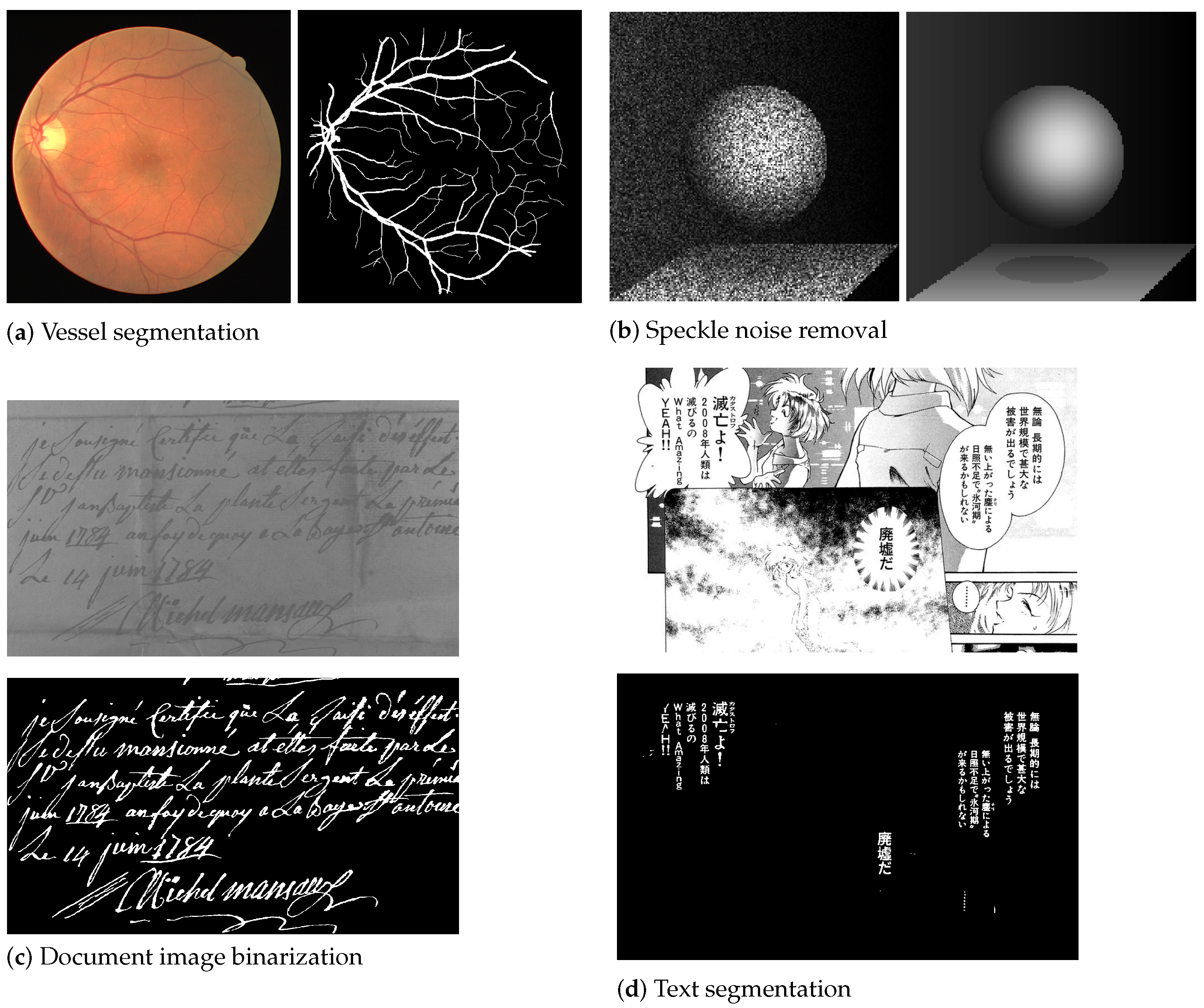
3.1. The Morphological Image Operator Learning Problem

We assume that images to be processed and respective expected transformed ones are realizations of a pair of random processes I × T with joint distribution P ( I , T ) . Given an image operator Ψ , one can measure how well Ψ can compute the target image T from an input image I by means of a loss function L ( Ψ ( I ) , T ) . The goal in image operator learning is to find an operator Ψ that minimizes the expected loss E [ L ( Ψ ( I ) , T ) ] , where expectation is computed with respect to distribution P. In practice, we assume that processes I × T are jointly stationary and the expected target image T of an input image I can be approximated reasonably well by some translation-invariant operator. Thus, the problem of designing image operators can be formulated as a problem of designing its characteristic function, defined on a support region W. Concerning binary images, in this formulation the observations are of the form ( I p W , T ( p ) ) , while for grayscale images they are of the form ( f p | W , T ( p ) ) . To simplify notation, from now on these observations will be denoted simply as ( x p , y p ) , without distinguishing whether they are binary or grayscale images. With this assumption, the relevant distribution is P ( x p , y p ) . It is commonly assumed that the same distribution holds for all locations p, and a single underlying distribution P ( x , y ) is then adopted. Thus, the loss of Ψ is expressed in terms of the loss of its characteristic function ψ , with respect to distribution P ( x , y ) .
Commonly used losses are the zero-one loss E [ ψ ( x ) y ] , the mean absolute error (MAE) E [ | ψ ( x ) y | ] , and the mean-square error (MSE) E [ ( ψ ( x ) y ) 2 ] . The estimator that minimizes the zero-one, MAE and MSE losses are, respectively, ψ ( x ) = arg max y K P ( y | x ) , ψ ( x ) = median of y | x , and ψ ( x ) = E [ y | x ] . For binary images (i.e., K = { 0 , 1 } ), these are all equivalent and thus the optimal operator is given by [21]:
ψ ( x ) = 1 , if P ( y = 1 | x ) > 0.5 , 0 , otherwise .
When the conditional probabilities P ( y = 1 | x ) are known, one could write down the interval operator for each or groups of patterns x and then express the local function as a maximum of these interval operators.

3.2. Learning Methods That Preserve Morphological Representation

Although one can formally characterize the optimal operator as discussed above, in practice the conditional probabilities P ( y | x ) are not known. Therefore, they are estimated by pooling data gathered from the training images. Training images are pairs as the ones shown in Figure 1. The target images usually need to be prepared manually. Initial approaches based on this statistical estimation setting were proposed by Dougherty [40,41], restricted to increasing operators, and then a general approach for increasing and non-increasing operators was proposed in [21]. From a machine-learning point of view, the method proposed in [21] can be seen as a two-step process. The first step is a fitting step, where optimal values y ^ = ψ ( x ) for observed patterns x , according to the chosen loss function, are computed based on the estimated probabilities P ^ ( y | x ) . The second step consists of a generalization step, when output values for non-observed patterns are defined. In [21], which deals with binary images only, a Boolean function minimization algorithm [42] is employed in the generalization step. More specifically, non-observed patterns are regarded as don’t-cares in the minimization process, and the resulting set of product terms (each corresponding to an interval) is such that it covers all patterns that satisfy y ^ = ψ ( x ) = 1 , does not cover any patterns that satisfy y ^ = ψ ( x ) = 0 , and may cover some of the don’t-cares. Please note that the resulting minimal sum-of-products expression corresponds to a basis representation of an operator. For grayscale images, decision-trees have been used [43]. In this case, each leaf node (that corresponds to an axis-parallel box) can be associated with an interval operator and the resulting estimator be understood as a maximum of interval operators, although representation minimization has not been addressed in the work.
The approach delineated above quickly becomes computationally prohibitive as the support region W increases. To circumvent this limitation, iterative training approaches [44] as well as a method [22] inspired in stacked generalization [45] have been proposed. In [22], a multi-level approach, based on a greedy optimization strategy, in which several first-level operators are optimized individually, then their outputs are used as input for the second-level operators, which are again optimized individually, and so on for the successive levels, has been proposed. The combination of multiple operators has resemblance to ensemble methods used in machine learning. In the same way some ensemble methods use classifiers trained on different sets of features, the multi-level operator training method uses slightly distinct support region for individual operators. The catch is to use moderate size individual windows whose union is a larger region. Therefore, in this case, the ultimate representation learned by the method is a cascade of functions, each one represented as a sum-of-products form, and such that effectively, the final operator is defined on a larger support region.
Earlier, with roots in signal processing, median, order statistic [46], and stack filters [47] became popular in the 1980s due to their property of commuting with the threshold decomposition. It has been shown that these filters are particular cases of increasing morphological operators [48]. In fact, stack filters are the family of increasing morphological operators with flat structuring elements [7], and thus they are also expressed as a supremum of erosions. The threshold decomposition property refers to the fact that to compute the result of these filters, one can apply the filter to each of the binary cross-sections obtained by thresholding the input signal at different gray levels, and then stacking the results to obtain the same result as when the filter is applied on the original signal. This property allowed performing the filtering of grayscale signals through binary signal filtering. For instance, median filtering is a particular case of order statistic filtering, in which the observed values are ordered and the median rather than a specific order k element is chosen as the output. Using the stacking approach, one can compute order statistics on the binary cross-sections relying only on counting and avoiding the need to sort the observations to compute the output. This technique was particularly interesting at a time when available computing capacity was limited. Many algorithms have been proposed in the past for the design of these filters from training data [23,49,50,51], most based on heuristic algorithms. Training data ( x , y ) are collected from binary cross-sections and pooled together to compute the optimal increasing binary operator, which is applied on the individual cross-sections.
The above-described methods produce results that can be associated with the “shallow” representation structures (maximum of intervals or maximum of erosion) of operators. Another approach that has been employed in morphological image operator learning is based on genetic algorithms [52,53] or genetic programming [54] that generate morphological image operators with “deeper” representations. Genetic algorithm is a heuristic method employed to perform searches in non-structured search spaces. Typically, solutions of interest are modeled as chromosomes, encoding for instance a sequence of n erosions and/or dilations with structuring elements of size up to m × m . In this case, a chromosome can be modeled as a binary vector with n + n m m components, where the first n components indicate the type of the n operators (erosion or dilation) and the remaining n m m components describe the respective n flat structuring elements of size m × m . Then, an initial family of these type of vectors are created and, through mutation and crossover operations, new valid vectors are generated, evolving to a new generation of operators. This process is repeated in such a way that the best fit individuals survive (measured by a fitness or loss function) from one generation to another, improving the overall population fitness along the iterations. After several iterations, the best fit individual is chosen at the end. Fitness is usually defined as some performance measure of the operator coded in the chromosome with respect to validation images. In genetic programming, possible solutions are built by composing building blocks according to pre-established rules. Thus, if one chooses a rich set of building blocks and composition rules, the space of all possible solutions may become very large. In [54], the authors employ binary erosions and dilation with a predefined set of possible structuring elements as the building blocks, and logical operations as composition rules.

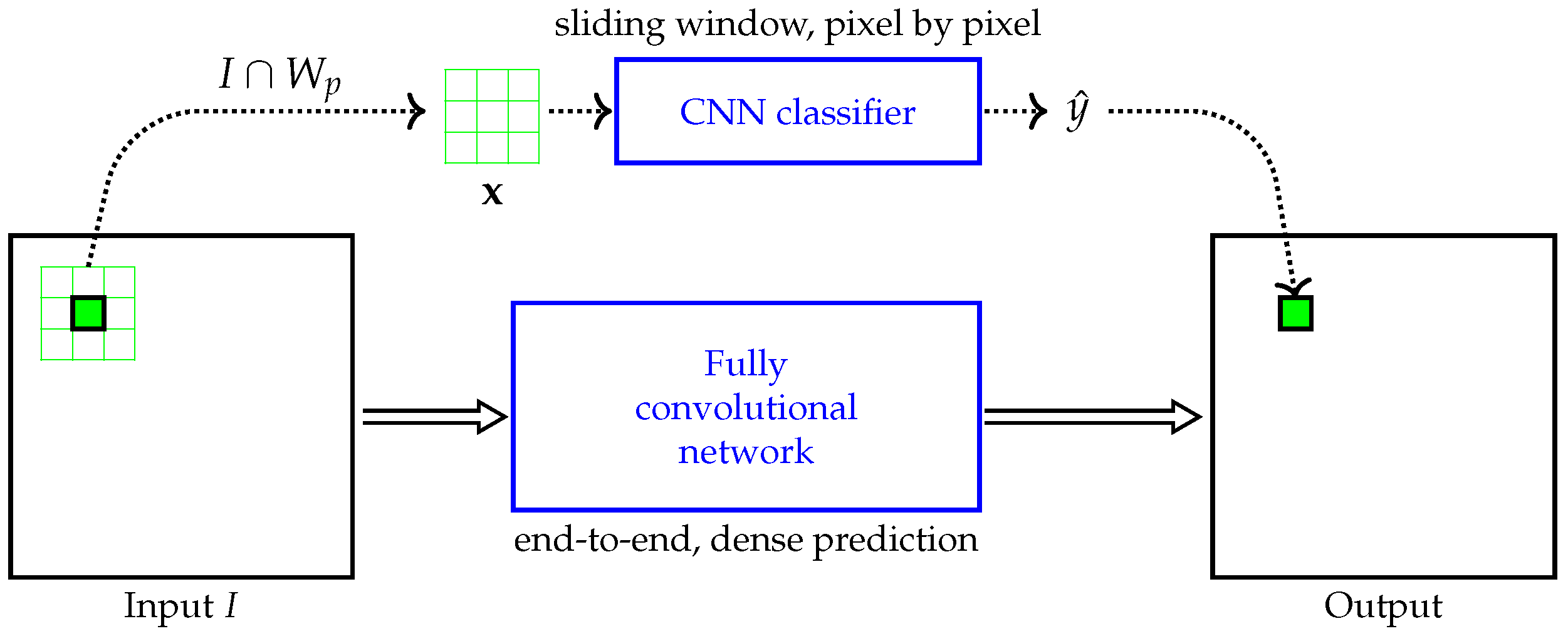
3.3. Links to Standard Machine Learning and Deep Learning

The characteristic function of an image operator is simply a function from K W to K. One can view the input images x in K W as a set of | W | features and the output values in K as class labels, as in standard classification problems. Therefore, if one is not concerned with representation aspects of such functions, in principle any classification algorithm can be used to learn these functions. In fact, the decision tree cited above is a popular algorithm used in general classification problems. In this section, we discuss learning approaches that have been developed completely detached from mathematical morphology. The general formulation, where the problem of learning image-to-image transformation is reduced to a simple pixel classification problem, can be summarized as illustrated in Figure 5. At the top part of the diagram is the standard approach of processing a vector representation of an image patch to predict the output value at its central pixel. Alternatively, as shown at the bottom part of the figure, rather than using the raw pixel intensities, one can create feature maps and extract a feature vector for each pixel. Along the years, a large effort was employed to extract discriminative features from the images, related to diverse cues such as gradients, texture, shape, among others [55,56,57,58]. The local region that effectively is used in the first case is defined by the image patch size, and in the second case it depends on the nature of the feature computation algorithm, and could be as large as the image size.
With modern deep neural networks, a significative advance was achieved regarding data representation learning. The origins of modern convolutional neural networks can be traced back to the 1980s [59,60]. The idea of shared weight neural networks was proposed in [60] and used for handwritten zip code recognition. While a standard feedforward network consists of a sequence of fully connected layers, a basic convolutional neural network (CNN) is a feedforward neural network consisting of convolutional layers, each followed by an activation function, possibly interspersed with pooling layers, and with fully connected layers at the end [60,61]. A convolutional layer is composed of neurons that compute a local computation commonly referred to as convolutions (although strictly speaking the implemented operations are cross-correlations, sum of point-wise multiplication), and characterized by a kernel. A same kernel is used to process every pixel in the input map, thus the connection between two adjacent layers is established only locally (meaning that the value of the output map at a given pixel depends only on the neighborhood of that pixel in the input map, delimited by the kernel size). In other words, each kernel in the convolutional layers of a CNN is applied on each pixel of the input map just as is the case of sliding window methods, but the processing is performed in parallel, based on efficient implementations using multidimensional arrays. The network is trained end-to-end and all weights of the network, including those of the kernels, are optimized during training using the gradient backpropagation algorithm [60,61].
In recent years, different architectures of CNN have been proposed for image classification tasks. Convolutional layers of CNNs are also used as backbone in network architectures designed for other types of tasks such as object recognition and semantic segmentation. As they process raw input images, it is commonly accepted that the convolutional layers work as feature extractors. This is paving modern machine learning, where efforts for manually crafting rich data representations is becoming non-essential.
In the context of image operator learning, two approaches that use CNNs have been proposed in the literature. The first consists of processing raw input image patches [62,63], as illustrated in the top part of the diagram in Figure 6. This can be compared to the bottom part of Figure 5, where classifiers are applied on extracted features. Here, with CNNs, feature extraction is learned during the training process. The second approach (bottom path in Figure 6) consists of fully convolutional networks. Networks of this type have no fully connected layers, allowing the processing of images of arbitrary size. These types of networks were initially proposed for semantic segmentation tasks [9,64] and later extended to image translations [65,66]. They usually consist of an encoding part (for instance a CNN) and a decoding part that takes care of restoring the original image size, as in U-Net [9].
These image-to-image networks have the advantage of computing the output image in a single forward pass. Nevertheless, the output value of a pixel is determined in terms of a receptive field, the region of the input image that is effectively used to compute the output value of that pixel, which can be understood as the support region of a local function. Therefore, ultimately these networks implicitly implement a nonlinear local function, and in this sense there is a connection to the morphological image operator learning problem discussed in this work.

4. Morphological Networks

Most recent advances regarding morphological image operator learning are related to deep morphological networks [25,26,27,28]. The key point of morphological neural networks (MNN) are neurons that compute erosions and dilations, which are nonlinear functions, in contrast to nodes of standard networks that typically compute a linear combination followed by a nonlinear activation. It is important to observe that there are two moments in MNN development. First, it was introduced in the 1990s as universal function approximation machines [67], just as the standard neural networks, and since then MNNs have been mostly used in general classification and regression problems. More recently, MNNs have been extended in the same way standard fully connected neural networks have been extended into convolutional neural networks (CNN). More specifically, in the extended MNNs, which hereafter will be called DMNN (Deep Morphological Neural Network), the morphological layers work as image feature extractors just like convolutional layers of CNNs [27,28].

4.1. Morphological Neural Networks

A neuron of a standard neural network computes a weighted linear combination of its input values. Let i be the index of a node in a given layer and suppose the output of the previous layer are a j , j = 1 , , n . The computation performed by node i is:
z i = ( j = 1 n a j w i j ) + b i
where w i j ( j = 1 , , n ) are weights and b i is a threshold also known as a bias. Typically, a nonlinear activation function θ generates the output of the neuron, a i = θ ( z i ) , which is sent to every node in the next layer.
Morphological neural networks (MNN) share a similar node structure, with the difference that the computation performed in the neurons is either an erosion or a dilation [67]:
z i = j = 1 n a j + w i j ( erosion )
z i = j = 1 n a j + w i j ( dilation )
While in standard neural networks the output z i is processed by a nonlinear activation function, in morphological neural networks there is no need for such processing because morphological operators are already nonlinear. Since its introduction, MNNs have been mostly employed as associative-memory machines or as binary or multiclass classifiers. For training these networks, most proposed methods are based on constructive algorithms [68]. An overview of the main developments of MNNs can be found in [69]. Methods based on standard stochastic gradient descent algorithm for training these networks have been discussed recently in [69,70].
Please note that in principle, MNNs could be also employed as classifiers in the learning scheme shown in Figure 5. Application of MNNs for image processing is not common, being mostly restricted to classification problems, applied on vector representation of the images. For instance, in [68] MNNs are used to classify pixels represented by a set of 19 features to solve an image segmentation problem. There are some exceptions, such as in [71] where morphological neural networks are applied to learn binary dilations, or in [72] where, inspired by convolutional layers of [60], the authors propose a neuron model that implements a gray-level hit-or-miss transform, and present an application in object detection, formulated as a template-matching problem.

4.2. Deep Morphological Networks

With recent advances in deep learning [73], pushed forward by the availability of large amounts of data, GPU-based efficient processing hardware, and open-source neural network libraries, there is a renewed interest in morphological neural networks in image processing. Next we present an overview of these recent models, the DMNNs (Deep Morphological Neural Networks), which take advantage of modern deep-learning frameworks to implement morphological layers (in a similar way convolutional layers are implemented in CNNs).

4.2.1. Morphological Neuron Modeling

To take advantage of existing deep-learning frameworks, an important detail is to have neurons implementing differentiable functions. Let us denote a general morphological neuron as M, which receives as input a signal x = ( x 1 , x 2 , , x n ) and has a weight vector w = ( w 1 , w 2 , , w n ) as a parameter. Its output is a scalar value M ( x ; w ) . In this case, the loss function to be optimized in the network training process must be differentiable with respect to each of the parameters w i , so that gradient descent-based methods can be employed to learn these weights. We review next, how this issue is addressed in three recent works. To that end, we use the notation just introduced. We use the 1-D notation for the sake of simplicity, but the same principles hold for the 2-D formulation used in image processing. In our notation, in the first morphological layer, input ( x 1 , x 2 , , x n ) would correspond to an image patch f | W p at some pixel p and, in subsequent morphological layers, it would correspond to a patch (of same size of W) in a feature map resulting from the previous layer computation. Parameters ( w 1 , w 2 , , w n ) correspond to the structuring function defined on a support region W, and M ( x ; w ) can be either the output of an erosion ε w ( x ) or of a dilation δ w ( x ) (actually M implements the characteristic function of an erosion or of a dilation).
Masci et al. [25] propose the use of the counter-harmonic mean as a function to compute approximations of erosions and dilations. The morphological neuron has an additional parameter P. Denoting x P the component-wise power to P of x , and assuming w is positive, a neuron is defined as:
M ( x ; w , P ) = x P + 1 w x P w
where ∗ is the standard convolution operation of CNNs. When P = 0 , the equation reduces to the usual convolution operation. When P tends to infinite, the right-hand side of the equation approaches the maximum of x (thus, dilation), and when P tends to minus infinite, it approaches the minimum of x (thus, erosion). Both parameters are learned during training, using the stochastic gradient descent algorithm. Then l o g ( w ) can be interpreted as a flat structuring function (in asymptotic sense).
Mondal et al. [27,70] and Franchi et al. [28] explore the fact that both erosion (minimum) and dilation (maximum) can be seen as piece-wise differentiable functions. The key point is to note that there is one input component x i that determines the output of node M and affects forward processing. Thus, during backpropagation, the gradient need to be back propagated only towards that input component.
In [27,28], the morphological formulation used is the same as the ones defined in Equations (10) and (11), which translated to the notation used in this section, is expressed as follows:
M ε ( x ; w ) = min i ( x i w i )
M δ ( x ; w ) = max i ( x n i + 1 + w i )
A dilation node M δ ( x ; w ) with input x and structuring function w affects the loss L through its output z + , Thus, the derivative of loss L with respect to w is computed as follows:
L w = L z + z + w
where L z + is the gradient backpropagated from the subsequent node and z + w is computed component-wise, for i = 1 , , n , as
z + w i = 1 , if M δ ( x ; w ) = x n i + 1 + w i , 0 , otherwise .
That is, there is one component of x (the maximum) that affects the loss L and therefore only its corresponding weight is updated.
Similar reasoning holds for the erosion nodes. Due to the difference in the definition of erosion and dilation, the component-wise derivative of erosion is either 0 or −1, while of the dilation is either 0 or 1. We also note that similar formulation is used in [72], to compute the gradient with respect to the weights of a hit-or-miss operator.

4.2.2. Types of Tasks and Architectures

Similarly to standard CNNs commonly used in classification tasks and fully convolutional networks in image-to-image transformation tasks, applications of DMNNs are also observed in these types of tasks.
A first natural idea to be explored in classification tasks would be to simply replicate some simple CNN architecture by replacing its convolutional layers with morphological layers. This is done in [26], where the morphological neuron modeling based on counter-harmonic-mean (Equation (19)) is used for classifying digits of the MNIST [8] and SVHN [74] datasets. For instance, for a simple CNN architecture consisting of one convolutional/morphological layer with 64 filters followed by a max pooling layer and a fully connected layer, authors show that the accuracy achieved on MNIST with standard CNN ( P = 0 in Equation (19)) is 98.7% while with morphological layers ( P = 2 in Equation (19)) is 99.07%. In [28], experiments regarding classification of images in MNIST [60] and CIFAR [75] datasets are described. However, in this second work the purpose is to demonstrate the potentials of morphological pooling layers used in place of conventional max pooling layers. The rationale for this replacement is based on the fact that max pooling can be interpreted as a dilation (since it computes the maximum) and therefore, rather than using a fixed pooling mask, it can be learned through a dilation operator. The authors report that by replacing the conventional pooling layers of common CNN architectures with morphological pooling layers, a slightly better result is achieved on MNIST [60] and CIFAR [75] datasets. These examples demonstrate that morphological neurons can be successfully trained using existing deep-learning frameworks. They also indicate that layers consisting of erosions or dilation nodes are effective in extracting representations that lead to good classification results. However, there is still no systematic comparison between standard CNNs and DMNNs for classification tasks reported in the literature.
With respect to image-to-image transformations, results regarding proof-of-concept tasks as well as some simple real image processing tasks are found in the literature. Proof-of-concept tasks consist of generating training images by applying relatively simple morphological operators, composed or not, with varying shapes for structuring functions, and then training deep morphological networks to learn these operators. In [25], a single layer single node network, with structuring function 11 × 11 , is used to learn erosions and dilations computed with structuring elements contained in the 5 × 5 square. Additionally, an architecture with two layers, each with a single node, is used to learn openings and closings. Due to the approximation nature of the morphological nodes (Equation (19)), results are slightly blurry although the shape of the learned structuring elements resembles those of the original structuring elements. The non-symmetric behavior of the approximations regarding parameter P is pointed as an issue, especially for learning erosions. These proof-of-concept experiments show that simple known morphological operators can be learned from data, although it should be noted that the network architecture definition may have been influenced by a prior knowledge of the target operator.
Regarding general image-to-image processing tasks as the ones illustrated in Figure 1, we summarize in Table 1 some of the tasks tackled using deep morphological networks in recent works. For details, we refer to the references listed in the table. These examples are still restricted to relatively simple processing and so far no systematic evaluation or comparison with CNNs has been reported. Nevertheless, the results indicate the potential of DMNNs for learning image transformations.

5. Discussion

With the current deep-learning frameworks, we are already able to build deep morphological neural network architectures (i.e., DMNNs) consisting of layers of morphological processing units, more precisely erosions and dilations, and take advantage of automatic gradient computation and weight optimization to learn the shape of the structuring functions. Concretely, this enables training of sequential compositions of morphological operators. Most of the experiments with DMNNs, reported in the literature, however, use hybrid architectures mixing morphological and convolutional layers, and so far experiments have been designed aiming for proof of concept rather than effectively solving image processing tasks. On the one hand, it is relatively simple to understand morphological layers as simple feature extractors, a role similar to that of convolutional layers. On the other hand, for image-to-image transformations, we still do not know very well how to specify and train a purely morphological network; for instance, it is not clear how multi-channel inputs should be handled or how to relate network size (number of layers and number of nodes in each layer) and its expressiveness.
Besides accuracy, interpretability and computational efficiency are two desirable characteristics of machine-learning algorithms. DMNNs have potential to fulfill these characteristics. In fact, if a neuron learns a structuring element, examination of the structuring element together with the operator type should be sufficient to provide an intuitive understanding of the processing performed by that particular node. For simple transformations such as opening or closing, some experiments reported in the literature show that DMNN can learn structuring functions with shape similar to the expected ones [25]. The fact that morphological operators are nonlinear functions creates an expectation that relatively small networks might be sufficient to learn complex image transformations. However, so far the number of reported results is not sufficient to draw conclusions regarding interpretability and computational efficiency.
Based on this discussion, we foresee some promising directions to be explored in future research regarding DMNN and its application in image processing problems.
  • Neurons that implement other morphological operators: Erosions and dilations are largely regarded as the building blocks of Mathematical Morphology. However, as we have seen, interval (hit-or-miss) operator is also a fundamental building block. This and possibly other operators could be implemented as morphological neurons, especially aiming more compact and expressive networks.
  • Development of standard architecture modules: Linear combination seems to be, so far, the most common way to compose the results regarding multiple input channels or multiple branches into a single result. Another possibility would be to perform composition using lattice operations such as supremum, infimum and negation. Such possibilities should be further investigated and developed. In particular, if we employ only morphological processing units and lattice operations, the whole network would correspond to a morphological expression, possibly improving its interpretability and further handling.
  • Hybrid networks: An obvious way to build hybrid networks is to use both convolutional as well as morphological layers in a single network, as already done in some of the reported experiments. However, there might be an optimal way of composing them, possibly, as distinct branches or modules within the architecture. In principle, there is no reason to assume that purely convolutional or purely morphological networks are preferable against the hybrid ones for a given task.
  • Systematic evaluation and comparison: Once some standard architectures become available, systematic evaluation and comparison should be performed among them as well as with convolution-based deep neural networks. This should include for instance networks of different sizes and multiple processing tasks.
  • Prior knowledge and regularization: In machine learning, the ability to constrain the space of predictor functions to a smaller space, without ruling out good predictors, is an important issue to improve generalization. Subfamilies of morphological image operators can be characterized based on properties such as idempotence, increasingness, anti-extensivity, and others. They can be also characterized in terms of representation; for instance, by limiting the number of intervals in the decomposition or constraining the structuring element shape. Thus, a challenging issue is how to translate prior knowledge about the task to be solved into appropriate constraints and how to enforce these constraints in the definition of the network architecture, as well as during the training process.
  • Iterative operators: Many useful morphological image operators such as thinning [20] are iterative applications of simpler operators, until convergence. Would recurrent network be the right approach to learn such operators?
  • Feature extraction process: On the one hand, there is an expectation that morphological neurons will reveal the nature of its processing more clearly than convolutional networks. On the other hand, they may end up just being an efficient data transformation function, not necessarily producing visually meaningful features. In this sense, it would be interesting to compare features extracted by convolutional layers and those extracted by morphological layers.
  • AutoML: Morphological pipelines designed heuristically to solve real image processing problems consist of a complex composition of multiple morphological operators. For learning such pipelines, rather than using a fixed network architecture, it may make more sense to experiment a variety of composition structures, much like the way genetic programming algorithms perform. In the deep-learning field, architecture search approaches are known as AutoML. For instance, approaches such as the one in [78] could be employed to build complex processing architectures, by combining morphological building block operators.

6. Conclusions

We presented a panorama on learning morphological image operators from training data. The fact that the definition of these operators is based on a solid theoretical foundation allows one to understand and explore their representations and properties (Section 2). In particular, many image transformations can be modeled by translation-invariant and locally defined operators, and thus the learning problem can be reduced to the problem of learning a local function defined on a small support region (Section 3).
Some learning approaches to design morphological image operators, and especially the earliest ones, explicitly keep the canonical morphological representation, and this facilitates interpretation or further manipulation of the learned operator (Section 3.2). However, as the optimization performed in the learning process involves solving combinatorial problems, for large support regions the optimization process becomes computationally intractable. To circumvent this, the local functions started to be treated as classifiers and standard machine-learning algorithms started to be employed. By doing so, one no longer has the explicit morphological representation. Moreover, if one uses CNNs as classifiers, not only there is no explicit morphological representation, but feature transformation is included in the learning process. Going one step further, instead of CNNs one can employ fully convolutional networks and then compute the output pixel values for the entire image in parallel (Section 3.3). Since image transformations computed by modern deep neural networks such as CNNs and fully convolutional networks are also translation-invariant and locally defined, there is a connection between morphological operators and convolution-based deep networks, but this connection is not explicit nor clear yet. On the other hand, deep neural networks implement compositions of simpler functions, which are jointly optimized. In morphological operator learning, before DMNNs there were no effective methods to jointly optimize structuring elements of a sequential composition of basic operators.
An important advance, thanks to deep-learning frameworks, is thus the possibility of optimizing the whole processing pipeline jointly, end-to-end, rather than step-by-step in a greedy fashion as done before. Although so far only relatively simple image processing tasks have been tackled with DMNNs, reported results provide evidence that they can be trained successfully. Systematic performance analysis of DMNNs or comparisons with CNNs are, however, still lacking in the literature. We still do not know the effort required for training these DMNNs in terms of processing time as well as amount of training data, or how training will work for larger networks or for more complex image transformations.
In summary, progress on morphological image operator learning along the years shows us a process that started strongly based on morphological representations (Section 3.2) and evolved to meet modern deep-learning techniques (Section 3.3), where no explicit trace of the morphological representation is seen. Currently, with DMNNs, we are witnessing the first steps of explicitly modeling morphological representations in the context of deep-learning techniques (Section 4). Some promising research directions in the context of DMNNs is listed in the previous section. Advances toward these directions should lead us to a better understanding with respect to expressiveness of compact DMNNs, interpretability, and potential of use in CPS applications.

Author Contributions

Conceptualization, N.S.T.H.; investigation, N.S.T.H. and G.A.P.; resources, N.S.T.H.; data curation, G.A.P.; writing–original draft preparation, N.S.T.H.; writing—review and editing, N.S.T.H. and G.A.P.; visualization, G.A.P.; supervision, N.S.T.H.; project administration, N.S.T.H.; funding acquisition, G.A.P. All authors have read and agreed to the published version of the manuscript.

Funding

This project has received funding from (a) the General Secretariat for Research and Technology (GSRT) of Greece by the “matching funds” of 2019 and (b) the European Union’s Horizon 2020 research and innovation programme under the Marie Skłodowska-Curie grant agreement No 777720. This work was also supported in part by the São Paulo Research Foundation (FAPESP) under grants number 2017/25835-9 and 2015/22308-2.

Institutional Review Board Statement

Not applicable.

Informed Consent Statement

Not applicable.

Data Availability Statement

Not applicable.

Conflicts of Interest

The authors declare no conflict of interest. The funders had no role in the design of the study; in the collection, analyses, or interpretation of data; in the writing of the manuscript, or in the decision to publish the results.

References

  1. Baheti, R.; Gill, H. Cyber-physical systems. Impact Control Technol. 2011, 12, 161–166. [Google Scholar]
  2. Sharma, A.B.; Ivančić, F.; Niculescu-Mizil, A.; Chen, H.; Jiang, G. Modeling and Analytics for Cyber-Physical Systems in the Age of Big Data. Sigmetr. Perform. Eval. Rev. 2014, 41, 74–77. [Google Scholar] [CrossRef]
  3. Garcia Lopez, P.; Montresor, A.; Epema, D.; Datta, A.; Higashino, T.; Iamnitchi, A.; Barcellos, M.; Felber, P.; Riviere, E. Edge-Centric Computing: Vision and Challenges. Sigcomm Comput. Commun. Rev. 2015, 45, 37–42. [Google Scholar] [CrossRef]
  4. Merenda, M.; Porcaro, C.; Iero, D. Edge Machine Learning for AI-Enabled IoT Devices: A Review. Sensors 2020, 20, 2533. [Google Scholar] [CrossRef] [PubMed]
  5. Maragos, P. Chapter Two—Representations for Morphological Image Operators and Analogies with Linear Operators. In Advances in Imaging and Electron Physics; Elsevier: Amsterdam, The Netherlands, 2013; Volume 177, pp. 45–187. [Google Scholar]
  6. Serra, J. Image Analysis and Mathematical Morphology; Academic Press: Cambridge, MA, USA, 1982. [Google Scholar]
  7. Heijmans, H.J.A.M. Morphological Image Operators; Academic Press: Boston, MA, USA, 1994. [Google Scholar]
  8. Lecun, Y.; Bottou, L.; Bengio, Y.; Haffner, P. Gradient-based learning applied to document recognition. Proc. IEEE 1998, 86, 2278–2324. [Google Scholar] [CrossRef] [Green Version]
  9. Ronneberger, O.; Fischer, P.; Brox, T. U-Net: Convolutional networks for biomedical image segmentation. In International Conference on Medical Image Computing and Computer-Assisted Intervention; Springer: Berlin/Heidelberg, Germany, 2015; pp. 234–241. [Google Scholar]
  10. Isola, P.; Zhu, J.; Zhou, T.; Efros, A.A. Image-to-Image Translation with Conditional Adversarial Networks. In Proceedings of the IEEE Conference on Computer Vision and Pattern Recognition (CVPR), Honolulu, HI, USA, 21–26 July 2017; pp. 5967–5976. [Google Scholar]
  11. Wen, W.; Wu, C.; Wang, Y.; Chen, Y.; Li, H. Learning Structured Sparsity in Deep Neural Networks. In Proceedings of the 30th Annual Conference on Neural Information Processing Systems 2016, Barcelona, Spain, 5–10 December 2016. [Google Scholar]
  12. Sze, V.; Chen, Y.; Yang, T.; Emer, J.S. Efficient Processing of Deep Neural Networks: A Tutorial and Survey. Proc. IEEE 2017, 105, 2295–2329. [Google Scholar] [CrossRef] [Green Version]
  13. Frankle, J.; Carbin, M. The Lottery Ticket Hypothesis: Finding Sparse, Trainable Neural Networks. In Proceedings of the Seventh International Conference on Learning Representations (ICLR: 2019), New Orleans, LA, USA, 6–9 May 2019. [Google Scholar]
  14. DRIVE: Digital Retinal Images for Vessel Extraction. Available online: https://drive.grand-challenge.org/ (accessed on 9 May 2021).
  15. Hedjam, R.; Cheriet, M. Historical document image restoration using multispectral imaging system. Pattern Recognit. 2013, 46, 2297–2312. [Google Scholar] [CrossRef]
  16. Hedjam, R.; Cheriet, M. Ground-Truth Estimation in Multispectral Representation Space: Application to Degraded Document Image Binarization. In Proceedings of the 12th International Conference on Document Analysis and Recognition, Washington, DC, USA, 25–28 August 2013; pp. 190–194. [Google Scholar]
  17. Aizawa, K.; Fujimoto, A.; Otsubo, A.; Ogawa, T.; Matsui, Y.; Tsubota, K.; Ikuta, H. Building a Manga Dataset “Manga109” with Annotations for Multimedia Applications. IEEE Multimed. 2020, 27, 8–18. [Google Scholar] [CrossRef]
  18. Matsui, Y.; Ito, K.; Aramaki, Y.; Fujimoto, A.; Ogawa, T.; Yamasaki, T.; Aizawa, K. Sketch-based Manga Retrieval using Manga109 Dataset. Multimed. Tools Appl. 2017, 76, 21811–21838. [Google Scholar] [CrossRef] [Green Version]
  19. Soille, P. Morphology Image Analysis, 2nd ed.; Springer: Berlin/Heidelberg, Germany, 2003. [Google Scholar]
  20. Dougherty, E.R.; Lotufo, R.A. Hands-on Morphological Image Processing; SPIE Press: Bellingham, WA, USA, 2003. [Google Scholar]
  21. Barrera, J.; Dougherty, E.R.; Tomita, N.S. Automatic Programming of Binary Morphological Machines by Design of Statistically Optimal Operators in the Context of Computational Learning Theory. Electron. Imaging 1997, 6, 54–67. [Google Scholar]
  22. Hirata, N.S.T. Multilevel Training of Binary Morphological Operators. IEEE Trans. Pattern Anal. Mach. Intell. 2009, 31, 707–720. [Google Scholar] [CrossRef] [PubMed]
  23. Dellamonica, D., Jr.; Silva, P.J.S.; Humes, C., Jr.; Hirata, N.S.T.; Barrera, J. An Exact Algorithm for Optimal MAE Stack Filter Design. IEEE Trans. Image Process. 2007, 16, 453–462. [Google Scholar] [CrossRef]
  24. Montagner, I.S.; Hirata, N.S.T.; Hirata, R., Jr. Staff removal using image operator learning. Pattern Recognit. 2017, 63, 310–320. [Google Scholar] [CrossRef]
  25. Masci, J.; Angulo, J.; Schmidhuber, J. A Learning Framework for Morphological Operators Using Counter—Harmonic Mean. In Mathematical Morphology and Its Applications to Signal and Image Processing; Hendriks, C.L.L., Borgefors, G., Strand, R., Eds.; Springer: Berlin/Heidelberg, Germany, 2013; pp. 329–340. [Google Scholar]
  26. Mellouli, D.; Hamdani, T.M.; Sanchez-Medina, J.J.; Ayed, M.B.; Alimi, A.M. Morphological Convolutional Neural Network Architecture for Digit Recognition. IEEE Trans. Neural Netw. Learn. Syst. 2019, 30, 2876–2885. [Google Scholar] [CrossRef] [PubMed]
  27. Mondal, R.; Purkait, P.; Santra, S.; Chanda, B. Morphological Networks for Image De-raining. In Discrete Geometry for Computer Imagery; Couprie, M., Cousty, J., Kenmochi, Y., Mustafa, N., Eds.; Springer: Berlin/Heidelberg, Germany, 2019; pp. 262–275. [Google Scholar]
  28. Franchi, G.; Fehri, A.; Yao, A. Deep morphological networks. Pattern Recognit. 2020, 102, 107246. [Google Scholar] [CrossRef]
  29. Matheron, G.; Serra, J. The birth of mathematical morphology. In Proceedings of the VIth International Symposium on Mathematical Morphology, Sydney, Australia, 3–5 April 2002; Talbot, H., Beare, R., Eds.; pp. 1–16. [Google Scholar]
  30. Serra, J. Image Analysis and Mathematical Morphology. Volume 2: Theoretical Advances; Academic Press: Cambridge, MA, USA, 1988. [Google Scholar]
  31. Maragos, P. A Representation Theory for Morphological Image and Signal Processing. IEEE Trans. Pattern Anal. Mach. Intell. 1989, 11, 586–599. [Google Scholar] [CrossRef]
  32. Maragos, P. Morphological Signal and Image Processing. In Digital Signal Processing Handbook; Madisetti, V., Williams, D., Eds.; CRC Press: Boca Raton, FL, USA, 1998; pp. 74:1–74:30. [Google Scholar]
  33. Banon, G.J.F.; Barrera, J. Minimal Representations for Translation-Invariant Set Mappings by Mathematical Morphology. SIAM J. Appl. Math. 1991, 51, 1782–1798. [Google Scholar] [CrossRef] [Green Version]
  34. Matheron, G. Random Sets and Integral Geometry; John Wiley: Hoboken, NJ, USA, 1975. [Google Scholar]
  35. Ross, K.A.; Wright, C.R.B. Discrete Mathematics, 3rd ed.; Prentice Hall: Hoboken, NJ, USA, 1992. [Google Scholar]
  36. Naegel, B.; Passat, N.; Ronse, C. Grey-Level Hit-or-Miss Transforms-Part I: Unified Theory. Pattern Recogn. 2007, 40, 635–647. [Google Scholar] [CrossRef] [Green Version]
  37. Ronse, C. A Lattice-Theoretical Morphological View on Template Extraction in Images. J. Vis. Commun. Image Represent. 1996, 7, 273–295. [Google Scholar] [CrossRef]
  38. Kaburlasos, V.G. Towards a Unified Modeling and Knowledge-Representation Based on Lattice Theory. In Computational Intelligence and Soft Computing Applications (Studies in Computational Intelligence); Springer: Berlin/Heidelberg, Germany, 2006; Volume 27. [Google Scholar]
  39. Kaburlasos, V.G. The Lattice Computing (LC) Paradigm. In Proceedings of the 15th International Conference on Concept Lattices and Their Applications (CLA), Tallinn, Estonia, 29 June–1 July 2020. [Google Scholar]
  40. Dougherty, E.R. Optimal Mean-Square N-Observation Digital Morphological Filters I. Optimal Binary Filters. CVGIP Image Underst. 1992, 55, 36–54. [Google Scholar] [CrossRef]
  41. Dougherty, E.R. Optimal Mean-Square N-Observation Digital Morphological Filters II. Optimal Gray-Scale Filters. CVGIP Image Underst. 1992, 55, 55–72. [Google Scholar] [CrossRef]
  42. Hirata, N.S.T.; Barrera, J.; Terada, R.; Dougherty, E.R. The Incremental Splitting of Intervals Algorithm for the Design of Binary Image Operators. In Proceedings of the 6th International Symposium: ISMM 2002, Sydney, Australia, 3–5 April 2002; Talbot, H., Beare, R., Eds.; pp. 219–228. [Google Scholar]
  43. Hirata, R., Jr.; Dougherty, E.R.; Barrera, J. Aperture Filters. Signal Process. 2000, 80, 697–721. [Google Scholar] [CrossRef]
  44. Hirata, N.S.T.; Dougherty, E.R.; Barrera, J. Iterative Design of Morphological Binary Image Operators. Opt. Eng. 2000, 39, 3106–3123. [Google Scholar]
  45. Wolpert, D.H. Stacked Generalization. Neural Netw. 1992, 5, 241–259. [Google Scholar] [CrossRef]
  46. Pitas, I.; Venetsanopoulos, A.N. Order statistics in digital image processing. Proc. IEEE 1992, 80, 1893–1921. [Google Scholar] [CrossRef] [Green Version]
  47. Wendt, P.D.; Coyle, E.J.; Gallagher, N.C., Jr. Stack Filters. IEEE Trans. Acoust. Speech Signal Process. 1986, ASSP-34, 898–911. [Google Scholar] [CrossRef]
  48. Maragos, P.; Schafer, R.W. Morphological Filters: Part II: Their Relations to Median, Order Statistic, and Stack-Filters. IEEE Trans. Acoust. Speech Signal Process. 1987, ASSP-35, 1170–1184. [Google Scholar] [CrossRef] [Green Version]
  49. Coyle, E.J. Rank order operators and the mean absolute error criterion. IEEE Trans. Acoust. Speech Signal Process. 1988, 36, 63–76. [Google Scholar] [CrossRef]
  50. Coyle, E.J.; Lin, J.H. Stack Filters and the Mean Absolute Error Criterion. IEEE Trans. Acoust. Speech Signal Process. 1988, 36, 1244–1254. [Google Scholar] [CrossRef]
  51. Yoo, J.; Fong, K.L.; Huang, J.J.; Coyle, E.J.; Adams, G.B., III. A Fast Algorithm for Designing Stack Filters. IEEE Trans. Image Process. 1999, 8, 1014–1028. [Google Scholar] [PubMed]
  52. Harvey, N.R.; Marshall, S. The Use of Genetic Algorithms in Morphological Filter Design. Signal Process. Image Commun. 1996, 8, 55–71. [Google Scholar] [CrossRef]
  53. Yoda, I.; Yamamoto, K.; Yamada, H. Automatic Acquisition of Hierarchical Mathematical Morphology Procedures by Genetic Algorithms. Image Vis. Comput. 1999, 17, 749–760. [Google Scholar] [CrossRef]
  54. Quintana, M.I.; Poli, R.; Claridge, E. Morphological algorithm design for binary images using genetic programming. Genet. Program. Evolvable Mach. 2006, 7, 81–102. [Google Scholar] [CrossRef] [Green Version]
  55. Haralick, R.M.; Shanmugam, K.; Dinstein, I. Textural Features for Image Classification. IEEE Trans. Syst. Man Cybern. 1973, SMC-3, 610–621. [Google Scholar] [CrossRef] [Green Version]
  56. Viola, P.; Jones, M. Rapid object detection using a boosted cascade of simple features. In Proceedings of the 2001 IEEE Computer Society Conference on Computer Vision and Pattern Recognition, Kauai, HI, USA, 8–14 December 2001; Volume 1. [Google Scholar]
  57. Lowe, D.G. Distinctive Image Features from Scale-Invariant Keypoints. Int. J. Comput. Vis. 2004, 60, 91–110. [Google Scholar] [CrossRef]
  58. Dalal, N.; Triggs, B. Histograms of oriented gradients for human detection. In Proceedings of the IEEE Computer Society Conference on Computer Vision and Pattern Recognition (CVPR), San Diego, CA, USA, 20–25 June 2005; Volume 1, pp. 886–893. [Google Scholar]
  59. Fukushima, K.; Miyake, S. Neocognitron: A Self-Organizing Neural Network Model for a Mechanism of Visual Pattern Recognition. In Competition and Cooperation in Neural Nets; Amari, S.I., Arbib, M.A., Eds.; Springer: Berlin/Heidelberg, Germany, 1982; pp. 267–285. [Google Scholar]
  60. LeCun, Y.; Boser, B.; Denker, J.S.; Henderson, D.; Howard, R.E.; Hubbard, W.; Jackel, L.D. Backpropagation Applied to Handwritten Zip Code Recognition. Neural Comput. 1989, 1, 541–551. [Google Scholar] [CrossRef]
  61. CS231n: Convolutional Neural Networks for Visual Recognition. Available online: https://cs231n.github.io/ (accessed on 29 July 2020).
  62. Julca-Aguilar, F.D.; Hirata, N.S.T. Image operator learning coupled with CNN classification and its application to staff line removal. In Proceedings of the 14th IAPR International Conference on Document Analysis and Recognition (ICDAR), Kyoto, Japan, 9–15 November 2017; pp. 53–58. [Google Scholar]
  63. Cireşan, D.C.; Giusti, A.; Gambardella, L.M.; Schmidhuber, J. Deep Neural Networks Segment Neuronal Membranes in Electron Microscopy Images. In Proceedings of the International Conference on Neural Information Processing Systems, Lake Tahoe, NV, USA, 3–6 December 2012; pp. 2843–2851. [Google Scholar]
  64. Long, J.; Shelhamer, E.; Darrell, T. Fully convolutional networks for semantic segmentation. In Proceedings of the IEEE Conference on Computer Vision and Pattern Recognition, Boston, MA, USA, 7–12 June 2015; pp. 3431–3440. [Google Scholar]
  65. Chen, Q.; Xu, J.; Koltun, V. Fast Image Processing with Fully-Convolutional Networks. In Proceedings of the IEEE International Conference on Computer Vision (ICCV), IEEE Computer Society, Venice, Italy, 22–29 October 2017; pp. 2516–2525. [Google Scholar]
  66. Wang, C.; Xu, C.; Wang, C.; Tao, D. Perceptual Adversarial Networks for Image-to-Image Transformation. IEEE Trans. Image Process. 2018, 27, 4066–4079. [Google Scholar] [CrossRef] [Green Version]
  67. Ritter, G.X.; Sussner, P. An introduction to morphological neural networks. In Proceedings of the 13th International Conference on Pattern Recognition, Washington, DC, USA, 25–29 August 1996; Volume 4, pp. 709–717. [Google Scholar]
  68. Sussner, P.; Esmi, E.L. Constructive Morphological Neural Networks: Some Theoretical Aspects and Experimental Results in Classification. In Constructive Neural Networks; Franco, L., Elizondo, D.A., Jerez, J.M., Eds.; Springer: Berlin/Heidelberg, Germany, 2009; pp. 123–144. [Google Scholar] [CrossRef]
  69. Zamora, E.; Sossa, H. Dendrite morphological neurons trained by stochastic gradient descent. Neurocomputing 2017, 260, 420–431. [Google Scholar] [CrossRef]
  70. Mondal, R.; Santra, S.; Chanda, B. Dense Morphological Network: An Universal Function Approximator. arXiv 2019, arXiv:abs/1901.00109. [Google Scholar]
  71. Davidson, J.L.; Hummer, F. Morphology neural networks: An introduction with applications. Circuits Syst. Signal Process. 1993, 12, 177–210. [Google Scholar] [CrossRef]
  72. Won, Y.; Gader, P.D.; Coffield, P.C. Morphological shared-weight networks with applications to automatic target recognition. IEEE Trans. Neural Netw. 1997, 8, 1195–1203. [Google Scholar] [PubMed]
  73. Goodfellow, I.; Bengio, Y.; Courville, A. Deep Learning; MIT Press: Cambridge, MA, USA, 2016. [Google Scholar]
  74. Netzer, Y.; Wang, T.; Coates, A.; Bissacco, A.; Wu, B.; Ng, A.Y. Reading Digits in Natural Images with Unsupervised Feature Learning. In Proceedings of the NIPS 2011 Workshop on Deep Learning and Unsupervised Feature Learning, Granada, Spain, 16–17 December 2011. [Google Scholar]
  75. Krizhevsky, A. Learning Multiple Layers of Features from Tiny Images; Technical Report; University of Toronto: Toronto, ON, Canada, 2009. [Google Scholar]
  76. Fu, X.; Huang, J.; Ding, X.; Liao, Y.; Paisley, J. Clearing the Skies: A Deep Network Architecture for Single-Image Rain Removal. IEEE Trans. Image Process. 2017, 26, 2944–2956. [Google Scholar] [CrossRef] [PubMed] [Green Version]
  77. Mondal, R.; Chakraborty, D.; Chanda, B. Learning 2D Morphological Network for Old Document Image Binarization. In Proceedings of the International Conference on Document Analysis and Recognition (ICDAR), Sydney, Australia, 20–25 September 2019; pp. 65–70. [Google Scholar]
  78. Real, E.; Liang, C.; So, D.R.; Le, Q.V. AutoML-Zero: Evolving Machine Learning Algorithms From Scratch. arXiv 2020, arXiv:cs.LG/2003.03384. [Google Scholar]
Figure 1. Examples of image-to-image transformations. (a) [14], (b) synthetic data, (c) Synchromedia Multispectral Ancient Document Images Dataset–SMADI [15,16], (d) EvaLady ©Miyone Shi, from Manga109 dataset [17,18].
Mathematics 09 01854 g001
Figure 2. Let B = { 1 , 0 , 1 } Z . At the top is the input signal. At the middle is its erosion by B, and at the bottom is the opening. As it can be seen, the value of the opening [ γ B ( I ) ] ( p ) is determined from the values of I ( p 2 ) , I ( p 1 ) , I ( p ) , I ( p + 1 ) , I ( p + 2 ) .
Mathematics 09 01854 g002
Figure 3. Lattice of all binary functions f : { 0 , 1 } 2 { 0 , 1 } , which corresponds to the binary image morphological operators locally defined with respect to a window with two points.
Mathematics 09 01854 g003
Figure 4. Images on W = { 2 , 1 , 0 , 1 , 2 } that are in the kernel of γ B (with B = { 1 , 0 , 1 } ). We have K ( γ B ) = { 00111 , 01110 , 11100 , 01111 , 10111 , 11101 , 11110 , 11111 } and B ( γ B ) = { [ 00111 , 11111 ] , [ 01110 , 11111 ] , [ 11100 , 11111 ] } .
Mathematics 09 01854 g004
Figure 5. Classifier acting as a local function. Raw image patch used as input of the classifier (top pipeline). Feature vector extracted from feature maps as input of the classifier (bottom pipeline).
Mathematics 09 01854 g005
Figure 6. Image transformation using deep-learning techniques. A pixel-wise classifier based on CNN (top) and an image-to-image fully convolutional network (bottom).
Mathematics 09 01854 g006
Table 1. Summary of deep morphological network applications in image processing tasks. At the current moment, they are still mostly at the proof-of-concept level.
TaskArchitecture DetailsRemarks
Defect detection in steel surface images [25].Two morphological layers with two nodes each, followed by a convolutional layer and an absolute difference (with respect to input image). Morphological nodes are the ones defined in Equation (19) and thus only an approximation of erosions and dilations are computed.The ground-truth images were generated by applying white top-hat with a disk of size 5 and a black top-hat with a line of size 10 that have been verified to be useful to detect bright small spots as well as dark line-like structures that characterize possible defects.
Noise filtering [25] (1) Binomial noise (2) Salt-and-pepper (3) Additive Gaussian noise(1) Two morphological layers with single node each (filter size 5 × 5). (2) 4 morphological layers with single node each. (3) Two morphological layers with two filters each plus an averaging layer. Same observation of the above cell, regarding morphological nodes.Network results are compared with: (1) A 2 × 2 opening; (2) a closing followed by an opening by a 2 × 2 structuring element; (3) the total variation restoration. The trained networks performed better than the hand-crafted operators, except for case (3).
Noise filtering [28] Salt-and-pepper noiseA sequence of morphological layers with single node each, corresponding to the sequence opening-closing-opening.Results indicate that the filtering task can be learned.
Edge detection [28]A convolutional neural network with one learnable morphological pooling layer, thus a hybrid network.An edge enhancing pre-processing is performed on the input images. The example showcases the use of morphological pooling layers.
Detraining [27]Architectures with two branches, each consisting of a sequential composition of erosion and dilation nodes. The two branches are linearly combined at the end.The networks are trained and tested on a synthetic rainy image dataset made available in [76]. One of the networks, with 16,780 parameters, presents a similar performance to the one obtained with a U-Net with 6,110,773 parameters.
Document binarization [77]Erosion and dilation nodes on multi-channel inputs are defined considering a multi-channel structuring function that generates a one-channel feature map. Then a morphological block is defined as consisting of c 1 dilation and c 2 erosion nodes, followed by λ linear combination nodes of the c 1 + c 2 channels. A network is a sequence of such blocks, with sigmoid activation at the end.Competitive results, for instance, with those of runners-up in the ICDAR2017 Competition on Document Image Binarization are achieved.
Publisher’s Note: MDPI stays neutral with regard to jurisdictional claims in published maps and institutional affiliations.

