Power Spectral Density Analysis of Nanowire-Anchored Fluctuating Microbead Reveals a Double Lorentzian Distribution

Abstract

In this work, we investigate the properties of a stochastic model, in which two coupled degrees of freedom are subordinated to viscous, elastic, and also additive random forces. Our model, which builds on previous progress in Brownian motion theory, is designed to describe water-immersed microparticles connected to a cantilever nanowire prepared by polymerization using two-photon direct laser writing (TPP-DLW). The model focuses on insights into nanowires exhibiting viscoelastic behavior, which defines the specific conditions of the microbead. The nanowire bending is described by a three-parameter linear model. The theoretical model is studied from the point of view of the power spectrum density of Brownian fluctuations. Our approach also focuses on the potential energy equipartition, which determines random forcing parametrization. Analytical calculations are provided that result in a double-Lorentzian power density spectrum with two corner frequencies. The proposed model explained our preliminary experimental findings as a result of the use of regression analysis. Furthermore, an a posteriori form of regression efficiency evaluation was designed and applied to three typical spectral regions. The agreement of respective moments obtained by integration of regressed dependences as well as by summing experimental data was confirmed.

1. Introduction

Many of the problems addressed by current nanosciences can be traced back to statistical mechanics and the concept of fluctuations. Fundamental problems constantly arise in nanosciences that go beyond conventional findings, complementing the emphasis and motivations of statistical mechanics. Related fields, now broadly referred to as stochastic processes, continue to pose a mathematical challenge.

Stochastic oscillations of anchored mechanical systems immersed in fluidic media or kept in vacuum have attracted significant attention in the past and are important in many ways today. The Brownian motion of a millimeter-sized mirror suspended from a torsion wire was utilized by Kappler back in 1931 to measure the Avogadro constant [1]. The thermal fluctuations of resonant micron-scale mechanical oscillators have been studied extensively, mostly in connection with AFM (atomic force microscopy) cantilevers and MEMS-based (micro- electromechanical) resonators [2,3,4,5,6]. Thermal fluctuations of glass nanofibers and silicon nitride cantilevers have been used to characterize and calibrate such systems for single-molecule force measurements [7,8]. Brownian motion has also been used at a smaller scale in TPM (tethered particle motion) experiments to investigate the properties of linear macromolecules such as DNA [9,10,11]. In contrast, thermal noise represents the main disturbing and limiting factor in experiments that rely on highly sensitive mechanical and opto-mechanical systems. Examples are inertial sensors [12,13] as well as recently proposed gravitational-wave and dark matter sensors [14,15,16].

Under certain conditions, system noises and their corresponding statistical quantities can become valuable, measurable features of technological devices and measurement instruments. When a particle immersed in a dissipative medium is simultaneously exposed to thermal noise, it reaches an equilibrium state with time, which provides a good possibility to measure statistical properties. Mechanical system fluctuations may also be related to intrinsic damping mechanisms such as internal friction, thermoelastic losses, or losses to the anchor system. Theoretical and experimental interest may then be directed toward elucidating the relationships between damping strength and noise. The well-known “fluctuation-dissipation theorem”, which is also used in this work, addresses these general relationships.

The significance of the outputs of the monitored processes is clearly influenced by the equipment parameters and laboratory conditions. As a result, analytical methods differ. The power spectrum of thermal fluctuations can be derived for the case of damped harmonic oscillators [17], which is a good approximation for AFM cantilevers in liquids and gases [3]. The basic oscillator theory was modified by Saulson [17] to account for the thermal noise of mechanical systems, whose losses are dominated by processes occurring inside the material. High external dissipation conditions represent another extreme, which usually happens for low-stiffness micron-scale [7] or even smaller (molecular) systems [18]. When immersed in viscous liquids, these structures operate in a non-resonant, overdamped regime. Interestingly, the same overdamping conditions are present in optical tweezers experiments, where the fluctuation theory was elaborated thoroughly [19,20].

In this work, we investigate the thermal fluctuations of micron-scale viscoelastic mechanical systems submerged in water. In this particular case, as we show below, both the dissipation to the surrounding fluid and the intrinsic damping play an important role.

We are interested in the stochastic motion of microbeads attached to cantilevered photopolymer nanowires prepared by two-photon polymerization direct laser writing (TPP-DLW) (see Figure 1a,b) [21,22]. The nanowire thickness can be tuned during the fabrication process [23]. In the limiting case of thin nanowires, the stochastic thermal forces exerted on the microbeads cause clearly detectable Brownian motion behavior (see Figure 1c), specifically in the direction perpendicular to the nanowire axis, as depicted in Figure 1d). Moreover, as recently demonstrated, photopolymer nanowires possess viscoelastic material properties [24,25], which define the specific confinement forces investigated in the present work.

Our present work is closely related to the preceding study focused on the bending recovery motion of photopolymer microbead-nanowire systems [25]. A three-parameter linear mechanical model of viscoelastic behavior has been found to provide a good explanation of the recovery time-dependence in this study. We aim to use the above theoretical description to include the thermal motion of the microstructure. This can be done analogously to other works. The original mechanistic model, which was first developed and validated in [25], can be generalized to reflect random forces. The problem can then be solved using the Fourier transform within the limits of the stochastic steady state in accordance with the experimental setup. The aim is to obtain the corresponding power spectrum and autocorrelation function of Brownian motions of the microstructure analytically. To summarize, our present approach promotes a practical and empirically supported transition from deterministic to stochastic frameworks.

2. Initial Considerations and Model Assumptions

Our main objective is to describe the stochastic motion of viscoelastic microstructures composed of cantilevered nanowires and spherical beads (see Figure 1) immersed in Newtonian liquids. The 18 $\mathsf{\mu }\mathrm{m}$ long nanowire equipped with a 5 $\mathsf{\mu }\mathrm{m}$ sphere (both made of Ormocomp) was prepared in a similar way as described in [25]. The previous work also provides all relevant experimental details. We assume that the nanowire bending is characterized by a 3-parameter linear mechanical model of viscoelastic behavior ( see Figure 2). In the thin nanowire limit, the external viscous damping and the external thermal forces acting on the nanowire itself are neglected. In this approximation, the liquid surroundings interact only with the attached bead. We focus our attention on the nanowire bending oscillations in the horizontal plane perpendicular to the nanowire axis (see Figure 1d).

The equivalent mechanical model, which consists of ideal spring and dashpot elements (shown in Figure 2), contains two parts. The left branch (A) stands for the nanowire forces exerted on the microbead. The photopolymer viscoelastic properties are characterized by the two elastic terms $k_1$, $k_2$ and the viscoelastic damping coefficient $\delta$. The right branch (B) includes the damping of the surrounding medium, with $\gamma$ denoting the hydrodynamic resistance. The inertia of the particle and the displaced fluid are neglected. Therefore, the results obtained represent a low-frequency approximation [20].

The basic mechanical model (i.e., model depicted in Figure 2, which is free of random forces $F_{\mathrm{T}1}=F_{\mathrm{T}2}=0$) is identical to the one given in [25]. This original form is amended here by adding stochastic forces to the system. In agreement with the fluctuation-dissipation theorem, uncorrelated Gaussian random forces ($F_{\mathrm{T}1}$ and $F_{\mathrm{T}2}$) are introduced in parallel with the dissipative elements $\delta$ and $\gamma$. Due to random excitation terms, the two displacement coordinates $x_1$ and $x_2$ fluctuate stochastically, which translates to the overall microbead displacement $x=x_1+x_2$. Unlike $x_1$ and $x_2$, the value of x can be observed experimentally. The power spectral density and the autocorrelation function of the microbead stochastic oscillations are derived by solving the system of Langevin equations describing the proposed model.

Research Design

Technological advances in microprinting 3D polymer patterns can stimulate and motivate progress in the formulation of appropriate mathematical and physical models. In this paper, we present a research framework associated with advanced two-photon microfabrication that can be applied in both practical and theoretical directions. Linear relationships are used to characterize the viscous and elastic properties of micromechanical systems (microbead nanowire systems) operating under stochastic (thermal) dynamic conditions. To evaluate observable coordinate changes, digital data from a CMOS image sensor is processed. This data can be represented mathematically as a one-dimensional time series.

The present study is motivated by experimental results, which, after analyzing the power spectral densities of the corresponding time series, show a kind of double Lorentzian form. The double Lorentzian form of the spectrum appears to us as an attractive research problem but also as a feature that has not yet been explored under the experimental conditions described above.

We use a regression approach with an objective function containing position-dependent weights in the spectrum to compare the theoretical model with experiments and perform the best model parameter finding as well. In addition, our analysis focuses on a validation strategy based on comparisons of differently obtained spectral moments.

Our study reflects the assumption that statistical mechanics models can reveal efficient ways to parameterize optically fabricated systems that exhibit significant fluctuations due to their size.

3. Model

The model consisting of two first-order stochastic differential equations is obtained based on the following considerations: (i) the forces acting in the upper and lower part of branch A are equal, and (ii) the sum of branch A and branch B forces is zero. We study the stochastic system for two displacement coordinates

$$\begin{array}{ccc}\hfill \delta \frac{\mathrm{d}{x}_2}{\mathrm{d}t}+k_2{x}_2-k_1{x}_1& =& F_{\mathrm{T}1},\hfill \\ \hfill \gamma \left(\frac{\mathrm{d}{x}_1}{\mathrm{d}t}+\frac{\mathrm{d}{x}_2}{\mathrm{d}t}\right)+k_1{x}_1& =& F_{\mathrm{T}2}\hfill \end{array}$$

(1)

formulated for the uncorrelated stationary Gaussian and white noise in time t random forces $F_{\mathrm{T}1}\left(t\right)$, $F_{\mathrm{T}2}\left(t\right)$. In such a framework, a set of assumptions applies to the mean values

$$\begin{array}{ccc}& & \langle F_{\mathrm{T}1}\left(t\right)\rangle =0,\langle F_{\mathrm{T}2}\left(t\right)\rangle =0,\hfill \\ & & \langle F_{\mathrm{T}1}\left(t\right)F_{\mathrm{T}2}(t+t^{\prime })\rangle =0\mathrm{for}\mathrm{all}t,t^{\prime };\hfill \\ & & \langle F_{\mathrm{T}1}\left(t\right)F_{\mathrm{T}1}(t+t^{\prime })\rangle =C_{\mathrm{FT}1}\widehat{\delta }\left(t^{\prime }\right),\hfill \\ & & \langle F_{\mathrm{T}2}\left(t\right)F_{\mathrm{T}2}(t+t^{\prime })\rangle =C_{\mathrm{FT}2}\widehat{\delta }\left(t^{\prime }\right)\hfill \end{array}$$

(2)

written by means of the Dirac delta function $\widehat{\delta }(.)$ (Here, the label $\widehat{\delta }$ is selected to distinguish it from the parameter $\delta$). The details and the physical rationale regarding the new parameter pair $C_{\mathrm{FT}1}$, $C_{\mathrm{FT}2}$ will be provided later in Section 4.3. To indicate the mean value in the space of repetitive random variants, we use the symbol $\langle \dots \rangle$, which is identified with the physical literature. Important here is the mathematical note that random forces are the derivatives of the corresponding Wiener processes.

4. Results

4.1. Solution of the Stochastic Problem

Using a linear transformation involving multiplication by the terms $1/\delta$, $1/\gamma$, as well as subtraction to remove the combination of derivatives on the left-hand side, we obtained a more standard form of the stochastic differential equation

$$\begin{array}{ccc}\hfill \left[\frac{\mathrm{d}}{\mathrm{d}t}+k_1\left(\frac{1}{\gamma }+\frac{1}{\delta }\right)\right]x_1-\frac{k_2}{\delta }{x}_2& =& F_{\mathrm{S}1},\hfill \\ & & \hfill \\ \hfill \left(\frac{\mathrm{d}}{\mathrm{d}t}+\frac{k_2}{\delta }\right)x_2-\frac{k_1}{\delta }{x}_1& =& F_{\mathrm{S}2},\hfill \end{array}$$

(3)

where the respective dissipative terms ($\sim \mathrm{d}{x}_1/\mathrm{d}t,$ $\sim \mathrm{d}{x}_2/\mathrm{d}t$) are counterbalanced by the auxiliary random forces $F_{\mathrm{S}1}$, $F_{\mathrm{S}2}$. There are no more mixed derivatives of variables in one equation, which results in a qualitative change from white to colored noise. The properties of $F_{\mathrm{S}1}$, $F_{\mathrm{S}2}$ can be represented by the linear relations

$$\begin{array}{c}\hfill F_{\mathrm{S}1}\left(t\right)=\frac{F_{\mathrm{T}2}\left(t\right)}{\gamma }-\frac{F_{\mathrm{T}1}\left(t\right)}{\delta },F_{\mathrm{S}2}\left(t\right)=\frac{F_{\mathrm{T}1}\left(t\right)}{\delta }.\end{array}$$

(4)

For computational purposes, the system of Equation (3) is converted to the Fourier domain in a standard way. Fourier images (coefficients), which we begin to denote by a tilde become functions of the angular frequency $\omega$. Despite the fact that ${\dots }_{\left(\omega \right)}$ or $\dots \left(\omega \right)$ symbols implying frequency dependence may be redundant in the case of white noise, it emphasizes the dependence on $\omega$ for general reasons in other situations. It is also worth noting that the complex conjugate’s asterisk label appears after the transition to the Fourier representation. Assuming that cross-correlations of Fourier images ${\tilde{F}}_{\mathrm{T}1}$, ${\tilde{F}}_{\mathrm{T}2}$ vanish as a result of Equations (2) and (4), for the relations of the first and the second-order moments, we have

$$\begin{array}{ccc}\hfill {\langle {\tilde{F}}_{\mathrm{S}1}\rangle }_{\left(\omega \right)}& =& {\langle {\tilde{F}}_{\mathrm{S}2}\rangle }_{\left(\omega \right)}=0,\hfill \\ \hfill {\langle {\tilde{F}}_{\mathrm{S}1}^{*}{\tilde{F}}_{\mathrm{S}1}\rangle }_{\left(\omega \right)}& =& \frac{1}{{\gamma }^2}{\langle {\tilde{F}}_{\mathrm{T}2}^{*}{\tilde{F}}_{\mathrm{T}2}\rangle }_{\left(\omega \right)}+\frac{1}{{\delta }^2}{\langle {\tilde{F}}_{\mathrm{T}1}^{*}{\tilde{F}}_{\mathrm{T}1}\rangle }_{\left(\omega \right)},\hfill \\ \hfill {\langle {\tilde{F}}_{\mathrm{S}2}^{*}{\tilde{F}}_{\mathrm{S}2}\rangle }_{\left(\omega \right)}& =& \frac{1}{{\delta }^2}{\langle {\tilde{F}}_{\mathrm{T}1}^{*}{\tilde{F}}_{\mathrm{T}1}\rangle }_{\left(\omega \right)},\hfill \\ \hfill {\langle {\tilde{F}}_{\mathrm{S}1}^{*}{\tilde{F}}_{\mathrm{S}2}\rangle }_{\left(\omega \right)}& =& {\langle {\tilde{F}}_{\mathrm{S}2}^{*}{\tilde{F}}_{\mathrm{S}1}\rangle }_{\left(\omega \right)}=-\frac{1}{{\delta }^2}{\langle {\tilde{F}}_{\mathrm{T}1}^{*}{\tilde{F}}_{\mathrm{T}1}\rangle }_{\left(\omega \right)}.\hfill \end{array}$$

(5)

Of course, the properties of the above averages are sufficient to determine multivariate Gaussian random force statistics. More precisely, the consequences of the Gaussian process from the postulates for $F_{\mathrm{T}1,2}$ towards the statements for $F_{\mathrm{S}1,2}$ can be easily justified.

According to the Equation (3), the respective coefficients ${\tilde{x}}_1\left(\omega \right)$, ${\tilde{x}}_2\left(\omega \right)$, ${\tilde{F}}_{\mathrm{S}1}\left(\omega \right)$, ${\tilde{F}}_{\mathrm{S}2}\left(\omega \right)$ are present in

$$\begin{array}{ccc}\hfill \mathbf{G}\left(\omega \right)\left(\begin{array}{c}{\tilde{x}}_1\left(\omega \right)\hfill \\ {\tilde{x}}_2\left(\omega \right)\hfill \end{array}\right)& =& \left(\begin{array}{c}{\tilde{F}}_{\mathrm{S}1}\left(\omega \right)\hfill \\ {\tilde{F}}_{\mathrm{S}2}\left(\omega \right)\hfill \end{array}\right),\hfill \end{array}$$

(6)

where

$$\mathbf{G}\left(\omega \right)=\left[\begin{array}{cc}i\omega +k_1\left(\frac{1}{\gamma }+\frac{1}{\delta }\right)\hfill & -\frac{k_2}{\delta }\hfill \\ -\frac{k_1}{\delta }\hfill & i\omega +\frac{k_2}{\delta }\hfill \end{array}\right].$$

(7)

Note that here $\mathbf{G}\left(\omega \right)$ is the label of newly introduced $\omega$-dependent matrix. The linearity of the problem implies that the solution

$$\begin{array}{ccc}\hfill \left(\begin{array}{c}{\tilde{x}}_1\left(\omega \right)\hfill \\ {\tilde{x}}_2\left(\omega \right)\hfill \end{array}\right)& =& {\mathbf{G}}^{-1}\left(\omega \right)\left(\begin{array}{c}{\tilde{F}}_{\mathrm{S}1}\left(\omega \right)\hfill \\ {\tilde{F}}_{\mathrm{S}2}\left(\omega \right)\hfill \end{array}\right)\hfill \end{array}$$

(8)

can be expressed in the terms of the inverse matrix ${\mathbf{G}}^{-1}\left(\omega \right)$. The following elements of the matrix represent a solution of the linear response type

$$\begin{array}{cc}{\left({\mathbf{G}}^{-1}\right)}_{11}\left(\omega \right)=\frac{1}{\det \left(\mathbf{G}\right(\omega \left)\right)}\left(i\omega +\frac{k_2}{\delta }\right),\hfill & {\left({\mathbf{G}}^{-1}\right)}_{12}\left(\omega \right)=\frac{1}{\det \left(\mathbf{G}\right(\omega \left)\right)}\frac{k_2}{\delta },\hfill \\ \hfill & \\ {\left({\mathbf{G}}^{-1}\right)}_{21}\left(\omega \right)=\frac{1}{\det \left(\mathbf{G}\right(\omega \left)\right)}\frac{k_1}{\delta },\hfill & {\left({\mathbf{G}}^{-1}\right)}_{22}\left(\omega \right)=\frac{1}{\det \left(\mathbf{G}\right(\omega \left)\right)}\left[i\omega +k_1\left(\frac{1}{\gamma }+\frac{1}{\delta }\right)\right].\hfill \end{array}$$

(9)

We see that the formulas contain $\det \left(\mathbf{G}\right)$=${\mathcal{G}}_R+i{\mathcal{G}}_I$, in the form $1/\det \left(\mathbf{G}\right)$= $({\mathcal{G}}_R-i{\mathcal{G}}_I)/({\mathcal{G}}_R^2+{\mathcal{G}}_I^2)$ with the auxiliary real-valued components ${\mathcal{G}}_R\left(\omega \right)$ and ${\mathcal{G}}_I\left(\omega \right)$. We also state that

$$\begin{array}{c}\hfill {\mathcal{G}}_R\left(\omega \right)=-{\omega }^2+\frac{k_1{k}_2}{\gamma \delta },{\mathcal{G}}_I\left(\omega \right)=\omega \left[\frac{k_2}{\delta }+k_1\left(\frac{1}{\gamma }+\frac{1}{\delta }\right)\right].\end{array}$$

(10)

Next, we will use

$$\begin{array}{c}\hfill {\left(\det \left(\mathbf{G}\right)\right)}^{*}\det \left(\mathbf{G}\right)={\mathcal{G}}_R^2+{\mathcal{G}}_I^2\end{array}$$

(11)

often reflected in the results.

4.2. Statistical Averages, Responses to Random Perturbations

This section is about the change to mean values, which are important for the measurement process, interpretation, and data processing. Only the statistics of the sum ${\tilde{x}}_1\left(\omega \right)+{\tilde{x}}_2\left(\omega \right)$, not isolated ${\tilde{x}}_1\left(\omega \right)$, ${\tilde{x}}_2\left(\omega \right)$ is observable in the experiment and allows comparison with the model. Thus, for many aspects of the study, only the behavior of ${\tilde{x}}_1\left(\omega \right)+{\tilde{x}}_2\left(\omega \right)$ needs to be used to determine experimentally relevant correlations. To understand the statistics of x, we focus on the Fourier spectrum of autocorrelation function

$$\begin{array}{ccc}\hfill C_{xx}\left(\omega \right)& \equiv & \langle \left({\tilde{x}}_1^{*}\left(\omega \right)+{\tilde{x}}_2^{*}\left(\omega \right)\right)\left({\tilde{x}}_1\left(\omega \right)+{\tilde{x}}_2\left(\omega \right)\right)\rangle \hfill \\ & =& {\langle {\tilde{x}}_1^{*}{\tilde{x}}_1\rangle }_{\left(\omega \right)}+{\langle {\tilde{x}}_2^{*}{\tilde{x}}_2\rangle }_{\left(\omega \right)}+{\langle {\tilde{x}}_1^{*}{\tilde{x}}_2\rangle }_{\left(\omega \right)}+{\langle {\tilde{x}}_2^{*}{\tilde{x}}_1\rangle }_{\left(\omega \right)}.\hfill \end{array}$$

(12)

It is of course convenient to divide it into four independent terms. In the following, these are treated independently by means of Equation (8). Partial results (so far without an emphasis on the $\omega$ dependence) are

$$\begin{array}{ccc}\hfill \langle {\tilde{x}}_1^{*}{\tilde{x}}_1\rangle & =& {\left({\mathbf{G}}^{-1}\right)}_{11}^{*}{\left({\mathbf{G}}^{-1}\right)}_{11}\langle {\tilde{F}}_{\mathrm{S}1}^{*}{\tilde{F}}_{\mathrm{S}1}\rangle +{\left({\mathbf{G}}^{-1}\right)}_{11}^{*}{\left({\mathbf{G}}^{-1}\right)}_{12}\langle {\tilde{F}}_{\mathrm{S}1}^{*}{\tilde{F}}_{\mathrm{S}2}\rangle \hfill \\ & +& {\left({\mathbf{G}}^{-1}\right)}_{12}^{*}{\left({\mathbf{G}}^{-1}\right)}_{11}\langle {\tilde{F}}_{\mathrm{S}2}^{*}{\tilde{F}}_{\mathrm{S}1}\rangle +{\left({\mathbf{G}}^{-1}\right)}_{12}^{*}{\left({\mathbf{G}}^{-1}\right)}_{12}\langle {\tilde{F}}_{\mathrm{S}2}^{*}{\tilde{F}}_{\mathrm{S}2}\rangle ,\hfill \\ & & \hfill \\ \hfill \langle {\tilde{x}}_2^{*}{\tilde{x}}_2\rangle & =& {\left({\mathbf{G}}^{-1}\right)}_{21}^{*}{\left({\mathbf{G}}^{-1}\right)}_{21}\langle {\tilde{F}}_{\mathrm{S}1}^{*}{\tilde{F}}_{\mathrm{S}1}\rangle +{\left({\mathbf{G}}^{-1}\right)}_{21}^{*}{\left({\mathbf{G}}^{-1}\right)}_{22}\langle {\tilde{F}}_{\mathrm{S}1}^{*}{\tilde{F}}_{\mathrm{S}2}\rangle \hfill \\ & +& {\left({\mathbf{G}}^{-1}\right)}_{22}^{*}{\left({\mathbf{G}}^{-1}\right)}_{21}\langle {\tilde{F}}_{\mathrm{S}2}^{*}{\tilde{F}}_{\mathrm{S}1}\rangle +{\left({\mathbf{G}}^{-1}\right)}_{22}^{*}{\left({\mathbf{G}}^{-1}\right)}_{22}\langle {\tilde{F}}_{\mathrm{S}2}^{*}{\tilde{F}}_{\mathrm{S}2}\rangle ,\hfill \\ & & \hfill \\ \hfill \langle {\tilde{x}}_1^{*}{\tilde{x}}_2\rangle & =& {\left({\mathbf{G}}^{-1}\right)}_{11}^{*}{\left({\mathbf{G}}^{-1}\right)}_{21}\langle {\tilde{F}}_{\mathrm{S}1}^{*}{\tilde{F}}_{\mathrm{S}1}\rangle +{\left({\mathbf{G}}^{-1}\right)}_{11}^{*}{\left({\mathbf{G}}^{-1}\right)}_{22}\langle {\tilde{F}}_{\mathrm{S}1}^{*}{\tilde{F}}_{\mathrm{S}2}\rangle \hfill \\ & +& {\left({\mathbf{G}}^{-1}\right)}_{12}^{*}{\left({\mathbf{G}}^{-1}\right)}_{21}\langle {\tilde{F}}_{\mathrm{S}2}^{*}{\tilde{F}}_{\mathrm{S}1}\rangle +{\left({\mathbf{G}}^{-1}\right)}_{12}^{*}{\left({\mathbf{G}}^{-1}\right)}_{22}\langle {\tilde{F}}_{\mathrm{S}2}^{*}{\tilde{F}}_{\mathrm{S}2}\rangle ,\hfill \\ & & \hfill \\ \hfill \langle {\tilde{x}}_2^{*}{\tilde{x}}_1\rangle & =& {\left({\mathbf{G}}^{-1}\right)}_{21}^{*}{\left({\mathbf{G}}^{-1}\right)}_{11}\langle {\tilde{F}}_{\mathrm{S}1}^{*}{\tilde{F}}_{\mathrm{S}1}\rangle +{\left({\mathbf{G}}^{-1}\right)}_{21}^{*}{\left({\mathbf{G}}^{-1}\right)}_{12}\langle {\tilde{F}}_{\mathrm{S}1}^{*}{\tilde{F}}_{\mathrm{S}2}\rangle \hfill \\ & +& {\left({\mathbf{G}}^{-1}\right)}_{22}^{*}{\left({\mathbf{G}}^{-1}\right)}_{11}\langle {\tilde{F}}_{\mathrm{S}2}^{*}{\tilde{F}}_{\mathrm{S}1}\rangle +{\left({\mathbf{G}}^{-1}\right)}_{22}^{*}{\left({\mathbf{G}}^{-1}\right)}_{12}\langle {\tilde{F}}_{\mathrm{S}2}^{*}{\tilde{F}}_{\mathrm{S}2}\rangle .\hfill \end{array}$$

(13)

We can achieve a clearer relationship by including the correlations between the initially imposed random forces ${\tilde{F}}_{\mathrm{T}1}$ and ${\tilde{F}}_{\mathrm{T}2}$ from Equation (5). The pairwise correlations take the form

$$\begin{array}{c}\hfill \langle {\tilde{x}}_s^{*}{\tilde{x}}_m\rangle =\left(\frac{\langle {\tilde{F}}_{\mathrm{T}2}^{*}{\tilde{F}}_{\mathrm{T}2}\rangle }{{\gamma }^2}+\frac{\langle {\tilde{F}}_{\mathrm{T}1}^{*}{\tilde{F}}_{\mathrm{T}1}\rangle }{{\delta }^2}\right){\overline{\overline{g}}}_{1;s,m}+\frac{\langle {\tilde{F}}_{\mathrm{T}1}^{*}{\tilde{F}}_{\mathrm{T}1}\rangle }{{\delta }^2}{\overline{\overline{g}}}_{2;s,m}\end{array}$$

(14)

with $s\in \{1,2\}$; $m\in \{1,2\}$, which define the following eight coefficients

$$\begin{array}{ccc}\hfill {\overline{\overline{g}}}_{1;1,1}& =& {\widehat{g}}_{11,11},{\overline{\overline{g}}}_{2;1,1}={\widehat{g}}_{12,12}-{\widehat{g}}_{11,12}^{\mathrm{sym}},\hfill \\ \hfill {\overline{\overline{g}}}_{1;2,2}& =& {\widehat{g}}_{21,21},{\overline{\overline{g}}}_{2;2,2}={\widehat{g}}_{22,22}-{\widehat{g}}_{21,22}^{\mathrm{sym}},\hfill \\ \hfill {\overline{\overline{g}}}_{1;1,2}& =& {\widehat{g}}_{11,21},{\overline{\overline{g}}}_{2;1,2}={\widehat{g}}_{12,22}-{\widehat{g}}_{11,22}-{\widehat{g}}_{12,21},\hfill \\ \hfill {\overline{\overline{g}}}_{1;2,1}& =& {\widehat{g}}_{21,11},{\overline{\overline{g}}}_{2;2,1}={\widehat{g}}_{22,12}-{\widehat{g}}_{21,12}-{\widehat{g}}_{22,11}.\hfill \end{array}$$

(15)

For the relations above, we use a notation that also includes the auxiliary symbols ${\widehat{g}}_{ij,kl}$ and ${\widehat{g}}_{ij,kl}^{\mathrm{sym}}$. They are interrelated to the combinations ${\left({\mathbf{G}}^{-1}\right)}_{ij}^{*}$ ${\left({\mathbf{G}}^{-1}\right)}_{ij}$ of the prior ${\mathbf{G}}^{-1}$ terms

$$\begin{array}{c}\hfill {\widehat{g}}_{ij,kl}={\left({\mathbf{G}}^{-1}\right)}_{ij}^{*}{\left({\mathbf{G}}^{-1}\right)}_{kl},{\widehat{g}}_{ij,kl}^{\mathrm{sym}}={\widehat{g}}_{ij,kl}+{\widehat{g}}_{kl,ij}.\end{array}$$

(16)

Obviously, the emphasis on the symmetry ${\widehat{g}}_{ij,kl}^{\mathrm{sym}}$$={\widehat{g}}_{kl,ij}^{\mathrm{sym}}$ will help us to handle the complex numbers. Furthermore, we recognize that the identical pairs of indices provide that ${\widehat{g}}_{ij,ij}=(1/2){\widehat{g}}_{ij,ij}^{\mathrm{sym}}$. The advantage of the auxiliary notation by means of ${\widehat{g}}_{\dots }$ is that we obtain $C_{xx}$ from Equation (12) in the compact form

$$\begin{array}{ccc}\hfill C_{xx}& =& \frac{\langle {\tilde{F}}_{\mathrm{T}2}^{*}{\tilde{F}}_{\mathrm{T}2}\rangle }{{\gamma }^2}\left({\widehat{g}}_{11,11}+{\widehat{g}}_{21,21}+{\widehat{g}}_{11,21}^{\mathrm{sym}}\right)\hfill \\ & +& \frac{\langle {\tilde{F}}_{\mathrm{T}1}^{*}{\tilde{F}}_{\mathrm{T}1}\rangle }{{\delta }^2}\left({\widehat{g}}_{11,11}+{\widehat{g}}_{12,12}+{\widehat{g}}_{21,21}+{\widehat{g}}_{22,22}\right.\hfill \\ & +& \left.{\widehat{g}}_{11,21}^{\mathrm{sym}}+{\widehat{g}}_{12,22}^{\mathrm{sym}}-{\widehat{g}}_{11,12}^{\mathrm{sym}}-{\widehat{g}}_{21,22}^{\mathrm{sym}}-{\widehat{g}}_{11,22}^{\mathrm{sym}}-{\widehat{g}}_{12,21}^{\mathrm{sym}}\right).\hfill \end{array}$$

(17)

We continue the calculation to reveal the terms introduced by Equation (16)

$$\begin{array}{c}\hfill \begin{array}{cc}{\widehat{g}}_{11,11}=\frac{1}{{\mathcal{G}}_R^2+{\mathcal{G}}_I^2}\left[{\omega }^2+{\left(\frac{k_2}{\delta }\right)}^2\right],\hfill & {\widehat{g}}_{21,21}=\frac{1}{{\mathcal{G}}_R^2+{\mathcal{G}}_I^2}{\left(\frac{k_1}{\delta }\right)}^2,\hfill \\ {\widehat{g}}_{22,22}=\frac{1}{{\mathcal{G}}_R^2+{\mathcal{G}}_I^2}\left[{\omega }^2+k_1^2{\left(\frac{1}{\gamma }+\frac{1}{\delta }\right)}^2\right],\hfill & {\widehat{g}}_{12,12}=\frac{1}{{\mathcal{G}}_R^2+{\mathcal{G}}_I^2}{\left(\frac{k_2}{\delta }\right)}^2,\hfill \end{array}\end{array}$$

(18)

$$\begin{array}{c}\hfill \begin{array}{cc}{\widehat{g}}_{11,21}^{\mathrm{sym}}=\frac{1}{{\mathcal{G}}_R^2+{\mathcal{G}}_I^2}\left(\frac{2k_1{k}_2}{{\delta }^2}\right),\hfill & {\widehat{g}}_{12,22}^{\mathrm{sym}}=\frac{1}{{\mathcal{G}}_R^2+{\mathcal{G}}_I^2}\left(\frac{2k_2{k}_1}{\delta }\right)\left(\frac{1}{\gamma }+\frac{1}{\delta }\right),\hfill \\ {\widehat{g}}_{11,12}^{\mathrm{sym}}=\frac{1}{{\mathcal{G}}_R^2+{\mathcal{G}}_I^2}\left(\frac{2k_2^2}{{\delta }^2}\right),\hfill & {\widehat{g}}_{21,22}^{\mathrm{sym}}=\frac{1}{{\mathcal{G}}_R^2+{\mathcal{G}}_I^2}\left(\frac{2k_1^2}{\delta }\right)\left(\frac{1}{\gamma }+\frac{1}{\delta }\right),\hfill \\ {\widehat{g}}_{11,22}^{\mathrm{sym}}=\frac{1}{{\mathcal{G}}_R^2+{\mathcal{G}}_I^2}\left[2{\omega }^2+\frac{2k_1{k}_2}{\delta }\left(\frac{1}{\gamma }+\frac{1}{\delta }\right)\right],\hfill & {\widehat{g}}_{12,21}^{\mathrm{sym}}=\frac{1}{{\mathcal{G}}_R^2+{\mathcal{G}}_I^2}\left(\frac{2k_1{k}_2}{{\delta }^2}\right).\hfill \end{array}\end{array}$$

(19)

Note that we used ${\mathcal{G}}_R$ and ${\mathcal{G}}_I$ from Equation (10) to express the result. After substituting these elements into Equation (17), we come to the relation

$$C_{xx}\left(\omega \right)=\frac{1}{{\gamma }^2({\mathcal{G}}_R^2+{\mathcal{G}}_I^2)}\left\{\langle {\tilde{F}}_{\mathrm{T}2}^{*}{\tilde{F}}_{\mathrm{T}2}\rangle \left[{\omega }^2+{\left(\frac{k_1+k_2}{\delta }\right)}^2\right]+\langle {\tilde{F}}_{\mathrm{T}1}^{*}{\tilde{F}}_{\mathrm{T}1}\rangle {\left(\frac{k_1}{\delta }\right)}^2\right\},$$

(20)

which is important to derive measurable results. We will apply a similar procedure later to determine the pairwise correlations to prove the validity of the equipartition theorem.

4.3. Towards Fusing of Theory and Experiment

Suppose that there are two finite formal limits relevant for the obtaining of the power spectral density in the form

$$C_{\mathrm{FT}1}=\underset{T_{\mathrm{msr}}\to \infty }{lim}\frac{\langle {\tilde{F}}_{\mathrm{T}1}^{*}{\tilde{F}}_{\mathrm{T}1}\rangle }{T_{\mathrm{msr}}},C_{\mathrm{FT}2}=\underset{T_{\mathrm{msr}}\to \infty }{lim}\frac{\langle {\tilde{F}}_{\mathrm{T}2}^{*}{\tilde{F}}_{\mathrm{T}2}\rangle }{T_{\mathrm{msr}}}.$$

(21)

The formula is understood as a postulate, which introduces the duration of the measurement time $T_{\mathrm{msr}}$ [19] into a part of the procedure at the formal level. The correlations in the Fourier domain can be formally taken as infinite for frequency $f=\frac{\omega }{2\pi }\gg 1/T_{\mathrm{msr}}$. The formal nature of the limits given by Equation (21) makes it evident that considerations are not fully compatible with the Fourier framework because the measurement is dependent on assumptions about the large time ($T_{\mathrm{msr}}$) of the measurement.

The occurrence of $C_{\mathrm{FT}1}$ and $C_{\mathrm{FT}2}$ later in Equation (23) can be interpreted as the contribution of the power spectral densities of two random force variants given by the Wiener–Khinchin theorem

$$\underset{T_{\mathrm{msr}}\to \infty }{lim}\frac{\langle {\tilde{F}}_{\mathrm{T}j}^{*}{\tilde{F}}_{\mathrm{T}j}\rangle }{T_{\mathrm{msr}}}={\int }_{-\infty }^{\infty }\mathrm{d}{t}^{\prime }{e}^{-2\pi if{t}^{\prime }}\langle F_{\mathrm{T}j}\left(t\right)F_{\mathrm{T}j}(t+t^{\prime })\rangle =C_{\mathrm{FT}j}$$

(22)

considered for $j=1,2$ alternatives (see Equation (2), where the correlation function is defined and integrated). If we extend the application of the formal limit by dividing Equation (20) with $T_{\mathrm{msr}}$, we obtain the power spectrum density in the form

$$\begin{array}{ccc}\hfill S_{xx}\left(f\right)& =& \underset{T_{\mathrm{msr}}\to \infty }{lim}\frac{C_{xx}\left(f\right)}{T_{\mathrm{msr}}}\hfill \\ & =& \frac{1}{{\gamma }^2{({\mathcal{G}}_R^2+{\mathcal{G}}_I^2)}_{\omega =2\pi f}}\left\{C_{\mathrm{FT}2}\left[4{\pi }^2{f}^2+{\left(\frac{k_1+k_2}{\delta }\right)}^2\right]+C_{\mathrm{FT}1}{\left(\frac{k_1}{\delta }\right)}^2\right\}.\hfill \end{array}$$

(23)

In this way, the physical meaning of the coefficients $C_{\mathrm{FT}1,2}$ is revealed. They can also be represented in an independent way by expressing their relation to the absolute temperature

$$C_{\mathrm{FT}1}=2k_{\mathrm{B}}T\delta ,C_{\mathrm{FT}2}=2k_{\mathrm{B}}T\gamma .$$

(24)

However, this construct also provides information about the dissipative mechanisms. This is built with the idea that fluctuations from random forces are dissipated by the mechanisms represented by the parameters $\delta$, $\gamma$. As provided below in Section 4.5, the mean potential energy for the respective degrees of freedom can be compared to determine the equilibrium level of energy flow controlled by $C_{\mathrm{FT}1}$ and $C_{\mathrm{FT}2}$. The Equation (24) given above is essentially the case of the general fluctuation–dissipation theorem introducing the natural heat unit $k_{\mathrm{B}}T$.

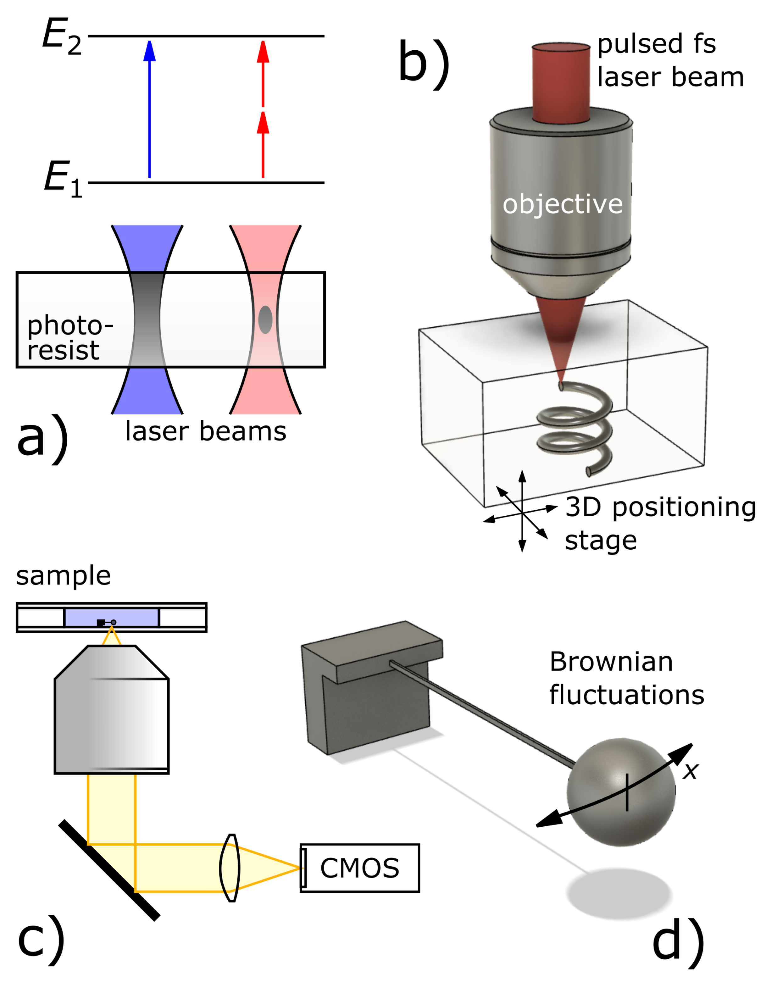
The fluctuation–dissipation theorem is a statistical thermodynamics statement that explains how fluctuations in a detailed balanced system determine its response to applied disturbances. According to this theorem, two opposing mechanisms are responsible for creating a detailed equilibrium in mechanical systems. On the one hand, there are the consequences of the dynamics of a microsphere attached to a nanowire that is damped by the surrounding fluid. Contributions from the internal damping mechanisms of the nanowire also fall into the same category. Even with this damping combination, the mechanical energy is converted into heat. On the other hand, the presence of damping is necessarily accompanied by fluctuations born in the viscous environment. In the case of the surrounding liquid, these fluctuations result in typical random Brownian collisions of liquid molecules with the microbead. In a standard way, the process is interpreted so that on microscopic scales, heat can be converted back into the mechanical energy of the microbead. The internal damping inside the nanowire acts likewise. Summarizing the above statements, we arrive at a specific form of the fluctuation-dissipation theorem, which states that a constant dissipation flux keeps the mean mechanical energy input invariant, while ensuring the production of new fluctuations.

As a result, let us emphasize an important point: Equation (23) can be modified to account for the temperature effect. With the intention of linking theory with experiment, we attain the expression

$$\begin{array}{c}\hfill S_{xx}\left(f\right)=\frac{2k_{\mathrm{B}}T}{\gamma }\frac{4{\pi }^2{f}^2+K_{\mathrm{A}}}{{\left(4{\pi }^2{f}^2-K_{\mathrm{B}}\right)}^2+4{\pi }^2{f}^2{K}_{\mathrm{C}}}.\end{array}$$

(25)

The asymptotic, high-frequency consequence of this general result is

$$S_{xx}\left(f\right)\simeq \frac{k_{B}T}{2{\pi }^2\gamma f^2},f\gg \frac{1}{2\pi }max\{\sqrt{K_{\mathrm{A}}},\sqrt{K_{\mathrm{B}}},\sqrt{K_{\mathrm{C}}}\}.$$

(26)

At this stage, we benefit from the choice of auxiliary parameters $K_{\mathrm{A}},K_{\mathrm{B}},K_{\mathrm{C}}$. Returning to material details is possible using transformations

$$K_{\mathrm{A}}={\left(\frac{k_1+k_2}{\delta }\right)}^2+\frac{\gamma }{\delta }{\left(\frac{k_1}{\gamma }\right)}^2,K_{\mathrm{B}}=\frac{k_1{k}_2}{\gamma \delta },K_{\mathrm{C}}={\left[\frac{k_2}{\delta }+k_1\left(\frac{1}{\gamma }+\frac{1}{\delta }\right)\right]}^2.$$

(27)

These auxiliary parameters are positive for a given model specification that operates exclusively with positive $k_1,k_2,\delta ,\gamma$. However, there is also another, more sophisticated level of interpretation. It is interesting and also productive to assume that the result can be written as a sum of two weighted Lorentzian functions

$$\begin{array}{ccc}\hfill \frac{4{\pi }^2{f}^2+K_{\mathrm{A}}}{{\left(4{\pi }^2{f}^2-K_{\mathrm{B}}\right)}^2+4{\pi }^2{f}^2{K}_{\mathrm{C}}}& \stackrel{!}{=}& \frac{1}{{\Gamma }_2-{\Gamma }_1}\left(\frac{K_{\mathrm{A}}-{\Gamma }_1}{{\Gamma }_1+4{\pi }^2{f}^2}+\frac{{\Gamma }_2-K_{\mathrm{A}}}{{\Gamma }_2+4{\pi }^2{f}^2}\right).\hfill \end{array}$$

(28)

Here ${\Gamma }_{1,2}$ play the role of free parameters, which incorporate information coming from previously introduced $K_{\mathrm{A}},$ $K_{\mathrm{B}}$, $K_{\mathrm{C}}$. The change to ${\Gamma }_{1,2}$ should be considered as an intermediate step along with other consequences. The key consequence is double Lorentzian form

$$S_{xx}\left(f\right)=\frac{k_{\mathrm{B}}T}{2{\pi }^2\gamma (f_{\mathrm{C}2}^2-f_{\mathrm{C}1}^2)}\left(\frac{\frac{K_{\mathrm{A}}}{4{\pi }^2}-f_{\mathrm{C}1}^2}{f_{\mathrm{C}1}^2+f^2}+\frac{f_{\mathrm{C}2}^2-\frac{K_{\mathrm{A}}}{4{\pi }^2}}{f_{\mathrm{C}2}^2+f^2}\right).$$

(29)

It is based on the assumption that there exist some relations between ${\Gamma }_{1,2}$ and the corner frequencies $f_{\mathrm{C}1,2}$. When Equations (28) and (29) are combined, we obtained

$$\begin{array}{c}\hfill f_{\mathrm{C}1,2}^2=\frac{{\Gamma }_{1,2}}{4{\pi }^2}=\frac{1}{4{\pi }^2}\left[\frac{K_{\mathrm{C}}}{2}-K_{\mathrm{B}}\mp \frac{1}{2}\sqrt{K_{\mathrm{C}}(K_{\mathrm{C}}-4K_{\mathrm{B}})}\right].\end{array}$$

(30)

In the above solution, we use the consensus that the plus sign corresponds to $f_{\mathrm{C}2}$. The constraints that allow for such a solution are as follows:

$$\frac{K_C}{2}-K_B\ge \frac{1}{2}\sqrt{K_{\mathrm{C}}(K_{\mathrm{C}}-4K_{\mathrm{B}})},K_{\mathrm{C}}\ge 0,K_{\mathrm{C}}\ge 4K_{\mathrm{B}}.$$

(31)

If we consider the transformation to physical parameters in the sense of Equation (27) to analyze the satisfaction of the above constraints, we obtain

$$\begin{array}{ccc}\hfill \frac{K_{\mathrm{C}}}{2}-K_{\mathrm{B}}& =& \frac{k_1^2}{2}{\left(\frac{1}{\gamma }+\frac{1}{\delta }\right)}^2+\frac{k_1{k}_2}{{\delta }^2}+\frac{k_2^2}{2{\delta }^2}\ge 0,\hfill \end{array}$$

(32)

$$\begin{array}{ccc}\hfill K_{\mathrm{C}}-4K_{\mathrm{B}}& =& {\left(\frac{k_2}{\delta }-\frac{k_1}{\gamma }\right)}^2+{\left(\frac{k_1}{\delta }\right)}^2+\frac{2k_1}{\delta }\left(\frac{k_2}{\delta }+\frac{k_1}{\gamma }\right)\ge 0.\hfill \end{array}$$

(33)

Using Equation (27), we confirm that $K_{\mathrm{C}}\ge 0$. Moreover, the trivial $K_{\mathrm{B}}^2\ge 0$ implies $(K_{\mathrm{C}}/2)-K_{\mathrm{B}}$≥$(1/2)$$\sqrt{K_{\mathrm{C}}(K_{\mathrm{C}}-4K_{\mathrm{B}})}$. Therefore, there is no obvious contradiction with the fact that ${\Gamma }_1$, ${\Gamma }_2$ correspond to $f_{\mathrm{C}1}^2$, $f_{\mathrm{C}2}^2$. It is also notable that the inverse transformations $(f_{\mathrm{C}1},f_{\mathrm{C}2})$→$({\Gamma }_1,{\Gamma }_2)$ →$(K_{\mathrm{B}},K_{\mathrm{C}})$ become

$$\begin{array}{ccc}\hfill K_{\mathrm{B}}& =& \sqrt{{\Gamma }_1{\Gamma }_2}=4{\pi }^2{f}_{\mathrm{C}1}{f}_{\mathrm{C}2},\hfill \\ \hfill K_{\mathrm{C}}& =& 2\left(\sqrt{{\Gamma }_1{\Gamma }_2}+\frac{{\Gamma }_1+{\Gamma }_2}{2}\right)=4{\pi }^2{\left(f_{\mathrm{C}1}+f_{\mathrm{C}2}\right)}^2.\hfill \end{array}$$

(34)

The result is intriguing in terms of revealing the central tendency in $K_{\mathrm{B}}({\Gamma }_1,{\Gamma }_2)$ and $K_{\mathrm{C}}({\Gamma }_1,{\Gamma }_2)$ as representatives of the pair ${\Gamma }_1$, ${\Gamma }_2$.

4.4. Autocorrelation Function

The findings presented above can be augmented by using direct time representation. According to the well-known Wiener–Khinchin relation, we have the consequence for the autocorrelation function in the form

$$R_{xx}\left(t\right)={\int }_{-\infty }^{\infty }\mathrm{d}f{S}_{xx}\left(f\right)exp\left(2\pi ift\right).$$

(35)

As a result, for Equation (29) as a specific version of $S_{xx}\left(f\right)$, we obtain a two-exponential autocorrelation function

$$\begin{array}{c}\hfill R_{xx}\left(t\right)={\mathcal{R}}_0\left({\mathcal{R}}_1{e}^{-2\pi f_{\mathrm{C}1}\left|t\right|}+{\mathcal{R}}_2{e}^{-2\pi f_{\mathrm{C}2}\left|t\right|}\right),\end{array}$$

(36)

where

$${\mathcal{R}}_0=\frac{k_{\mathrm{B}}T}{2\pi \gamma (f_{\mathrm{C}2}^2-f_{\mathrm{C}1}^2)},{\mathcal{R}}_1=\frac{\frac{K_{\mathrm{A}}}{4{\pi }^2}-f_{\mathrm{C}1}^2}{f_{\mathrm{C}1}},{\mathcal{R}}_2=\frac{f_{\mathrm{C}2}^2-\frac{K_{\mathrm{A}}}{4{\pi }^2}}{f_{\mathrm{C}2}}.$$

(37)

It is worth noting that corner frequency parameters have a significant impact on autocorrelation decrease over time. At a first glance, we can see the essential property here where a pair of frequencies in the Lorentz form corresponds to a pair of damping terms with the typical decay times proportional to $1/f_{\mathrm{C}1}$ and $1/f_{\mathrm{C}2}$. It should also be noted that, assuming that the physical parameters are constant, the temperature is directly manifested only in the amplitude ${\mathcal{R}}_0$. The calculations above were performed with the help of a well-known auxiliary relation

$${\int }_{-\infty }^{\infty }\mathrm{d}f\frac{exp\left(2\pi ift\right)}{f^2+f_{\mathrm{C}}^2}=\frac{\pi }{f_{\mathrm{C}}}exp\left(-2\pi \left|t\right|f_{\mathrm{C}}\right)$$

(38)

with some auxiliary parameter $f_{\mathrm{C}}$.

4.5. Sharing of Elastic Energy; Rationale for Choosing $C_{\mathrm{FT}1}$, $C_{\mathrm{FT}2}$

According to the principle of energy equipartition, average energy is evenly distributed among the various degrees of freedom of ergodic systems. As shown here, the implications of this principle are valuable tools for calculating the amplitudes $(C_{\mathrm{FT}1},C_{\mathrm{FT}2})$ of a pair of random forces. The equipartition principle can be applied to the mean elastic energies. We start by writing the energy for the Fourier modes corresponding to $\omega$. It is worth noting that since the inertial term is considered negligible, the zero limit of the kinetic energy has no effect on the equipartition issues.

Using the integration techniques already discussed, we continue to utilize the formal limit approach ($T_{\mathrm{mrs}}\to \infty$) for the integration of the spectrum and averaging over the respective potential energy fluctuations as follows

$$\begin{array}{ccc}\hfill U_{\mathrm{P}1}& =& \frac{k_1}{2}{\int }_0^{\infty }\mathrm{d}\omega {\langle {\tilde{x}}_1^{*}{\tilde{x}}_1\rangle }_{\left(\omega \right)}=I_{\mathrm{P}11}{C}_{\mathrm{FT}1}+I_{\mathrm{P}12}{C}_{\mathrm{FT}2},\hfill \\ \hfill U_{\mathrm{P}2}& =& \frac{k_2}{2}{\int }_0^{\infty }\mathrm{d}\omega {\langle {\tilde{x}}_2^{*}{\tilde{x}}_2\rangle }_{\left(\omega \right)}=I_{\mathrm{P}21}{C}_{\mathrm{FT}1}+I_{\mathrm{P}22}{C}_{\mathrm{FT}2}.\hfill \end{array}$$

(39)

The formulas below can be applied to complete the integration

$$\begin{array}{c}\hfill \begin{array}{cc}{I}_{\mathrm{P}11}=\frac{k_1}{2{\delta }^2}{I}_{\mathrm{E}2},\hfill & I_{\mathrm{P}12}=\frac{k_1}{2{\gamma }^2}\left[I_{\mathrm{E}2}+{\left(\frac{k_2}{\delta }\right)}^2{I}_{\mathrm{E}0}\right],\hfill \\ I_{\mathrm{P}21}=\frac{k_2}{2{\delta }^2}\left[I_{\mathrm{E}2}+{\left(\frac{k_1}{\gamma }\right)}^2{I}_{\mathrm{E}0}\right],\hfill & I_{\mathrm{P}22}=\frac{k_2{k}_1^2}{2{\gamma }^2{\delta }^2}{I}_{\mathrm{E}0}.\hfill \end{array}\end{array}$$

(40)

These four coefficients include two spectral integrals

$$I_{\mathrm{E}0}={\int }_0^{\infty }\frac{\mathrm{d}\omega }{\pi }\frac{1}{{\mathcal{G}}_R^2\left(\omega \right)+{\mathcal{G}}_I^2\left(\omega \right)},I_{\mathrm{E}2}={\int }_0^{\infty }\frac{\mathrm{d}\omega }{\pi }\frac{{\omega }^2}{{\mathcal{G}}_R^2\left(\omega \right)+{\mathcal{G}}_I^2\left(\omega \right)}.$$

(41)

Going back to a spectral decomposition using a pair of Lorentzian forms (see Equation (29)) in combination with Equations (30) and (34) gives the following result

$$\begin{array}{ccc}\hfill I_{\mathrm{E}0}& =& \frac{1}{2({\Gamma }_2-{\Gamma }_1)}\left(\frac{1}{\sqrt{{\Gamma }_1}}-\frac{1}{\sqrt{{\Gamma }_2}}\right)=\frac{1}{2K_{\mathrm{B}}\sqrt{K_{\mathrm{C}}}},\hfill \\ \hfill I_{\mathrm{E}2}& =& \frac{1}{2({\Gamma }_2-{\Gamma }_1)}\left(\sqrt{{\Gamma }_2}-\sqrt{{\Gamma }_1}\right)=\frac{1}{\sqrt{K_{\mathrm{C}}}}.\hfill \end{array}$$

(42)

As a consequence, the following relationship $I_{\mathrm{E}2}$ =$I_{\mathrm{E}0}$$k_1{k}_2$$/\left(\gamma \delta \right)$ can be used in the mean potential energies listed below

$$\begin{array}{ccc}\hfill U_{\mathrm{P}1}& =& \frac{k_1{k}_2}{2\gamma \delta }\left[\left(\frac{k_1}{\delta }\right)\frac{C_{\mathrm{FT}1}}{\delta }+\left(\frac{k_1}{\gamma }+\frac{k_2}{\delta }\right)\frac{C_{\mathrm{FT}2}}{\gamma }\right]I_{\mathrm{E}0},\hfill \\ \hfill U_{\mathrm{P}2}& =& \frac{k_1{k}_2}{2\gamma \delta }\left[\left(\frac{k_1}{\gamma }+\frac{k_2}{\delta }\right)\frac{C_{\mathrm{FT}1}}{\delta }+\left(\frac{k_1}{\delta }\right)\frac{C_{\mathrm{FT}2}}{\gamma }\right]I_{\mathrm{E}0}.\hfill \end{array}$$

(43)

Finally, in accordance with Equation (24), we have the confirmation of the equipartition in the form

$$U_{\mathrm{P}1}=U_{\mathrm{P}2}=K_{\mathrm{B}}\sqrt{K_{\mathrm{C}}}{I}_{\mathrm{E}0}{k}_{\mathrm{B}}T=\frac{1}{2}{k}_{\mathrm{B}}T.$$

(44)

4.6. The Spectrum Moments

In this subsection, we discuss the usefulness of introducing power spectral density integrals in cases where the frequency domain over which we integrate is divided into non-intersecting intervals. Frequency integration is motivated by the fact that providing excessive detail for spectrum characterization may be unnecessary in certain contexts. The second reason is that aggregation of data helps to suppress statistical errors. The third reason is the possibility of comparing only a few moments with the moments estimated by direct data processing.

Naturally, the analytical form of the model moments simplifies further processing. In our case, the specificity of the moments corresponding to Lorentzian and related spectral forms supports the overall validation process. Let the regression-related (rr) moments obtained by analytical integration be referred to as ${\mathcal{M}}_{\mathrm{Sxx}}^{\mathrm{rr}}(f_{\mathrm{L}},f_{\mathrm{H}})$. This notation is used to mean that integration has occurred within the range between the lowest $f_{\mathrm{L}}$ and the highest $f_{\mathrm{H}}$ frequencies. Then

$$\begin{array}{ccc}& & {\mathcal{M}}_{\mathrm{Sxx}}^{\mathrm{rr}}(f_{\mathrm{L}},f_{\mathrm{H}})={\int }_{f_{\mathrm{L}}}^{f_{\mathrm{H}}}\mathrm{d}f{S}_{xx}\left(f\right)\hfill \\ & & =\frac{{\mathcal{R}}_0}{\pi }\left[{\mathcal{R}}_1\left(arctan\left(\frac{f_{\mathrm{H}}}{f_{\mathrm{C}1}}\right)-arctan\left(\frac{f_{\mathrm{L}}}{f_{\mathrm{C}1}}\right)\right)\right.\hfill \\ & & +\left.{\mathcal{R}}_2\left(arctan\left(\frac{f_{\mathrm{H}}}{f_{\mathrm{C}2}}\right)-arctan\left(\frac{f_{\mathrm{L}}}{f_{\mathrm{C}2}}\right)\right)\right].\hfill \end{array}$$

(45)

Because the interval length may diverge, we decided to use non-normalized moments. Recall that ${\mathcal{R}}_1$ and ${\mathcal{R}}_2$ are the two respective amplitudes of the exponentials corresponding to the autocorrelation function (see Equation (37)). On this basis, using $f_{\mathrm{C}1}$, $f_{\mathrm{C}2}$ as natural boundaries, we can define the system of three specific regression-related spectral moments

$$\begin{array}{ccc}& & {\mathcal{M}}_{\mathrm{Sxx}}^{\mathrm{rr}}(0,f_{\mathrm{C}1})=\frac{{\mathcal{R}}_0}{\pi }\left[{\mathcal{R}}_1\frac{\pi }{4}+{\mathcal{R}}_{2}arctan\left(\frac{f_{\mathrm{C}1}}{f_{\mathrm{C}2}}\right)\right],\hfill \\ & & {\mathcal{M}}_{\mathrm{Sxx}}^{\mathrm{rr}}(f_{\mathrm{C}1},f_{\mathrm{C}2})=\frac{{\mathcal{R}}_0}{\pi }\left[{\mathcal{R}}_{1}arctan\left(\frac{f_{\mathrm{C}2}}{f_{\mathrm{C}1}}\right)-{\mathcal{R}}_{2}arctan\left(\frac{f_{\mathrm{C}1}}{f_{\mathrm{C}2}}\right)+({\mathcal{R}}_2-{\mathcal{R}}_1)\frac{\pi }{4}\right],\hfill \\ & & {\mathcal{M}}_{\mathrm{Sxx}}^{\mathrm{rr}}(f_{\mathrm{C}2},\infty )=\frac{{\mathcal{R}}_0}{\pi }\left[(2{\mathcal{R}}_1+{\mathcal{R}}_2)\frac{\pi }{4}-{\mathcal{R}}_{1}arctan\left(\frac{f_{\mathrm{C}2}}{f_{\mathrm{C}1}}\right)\right]\hfill \end{array}$$

(46)

with the total sum $(1/2){\mathcal{R}}_0$ $({\mathcal{R}}_1+{\mathcal{R}}_2)$. Other suitable boundary options are, of course, possible, such as those that do not depend on regression results but instead emerge entirely from generalized averaging procedures of the experimental spectrum.

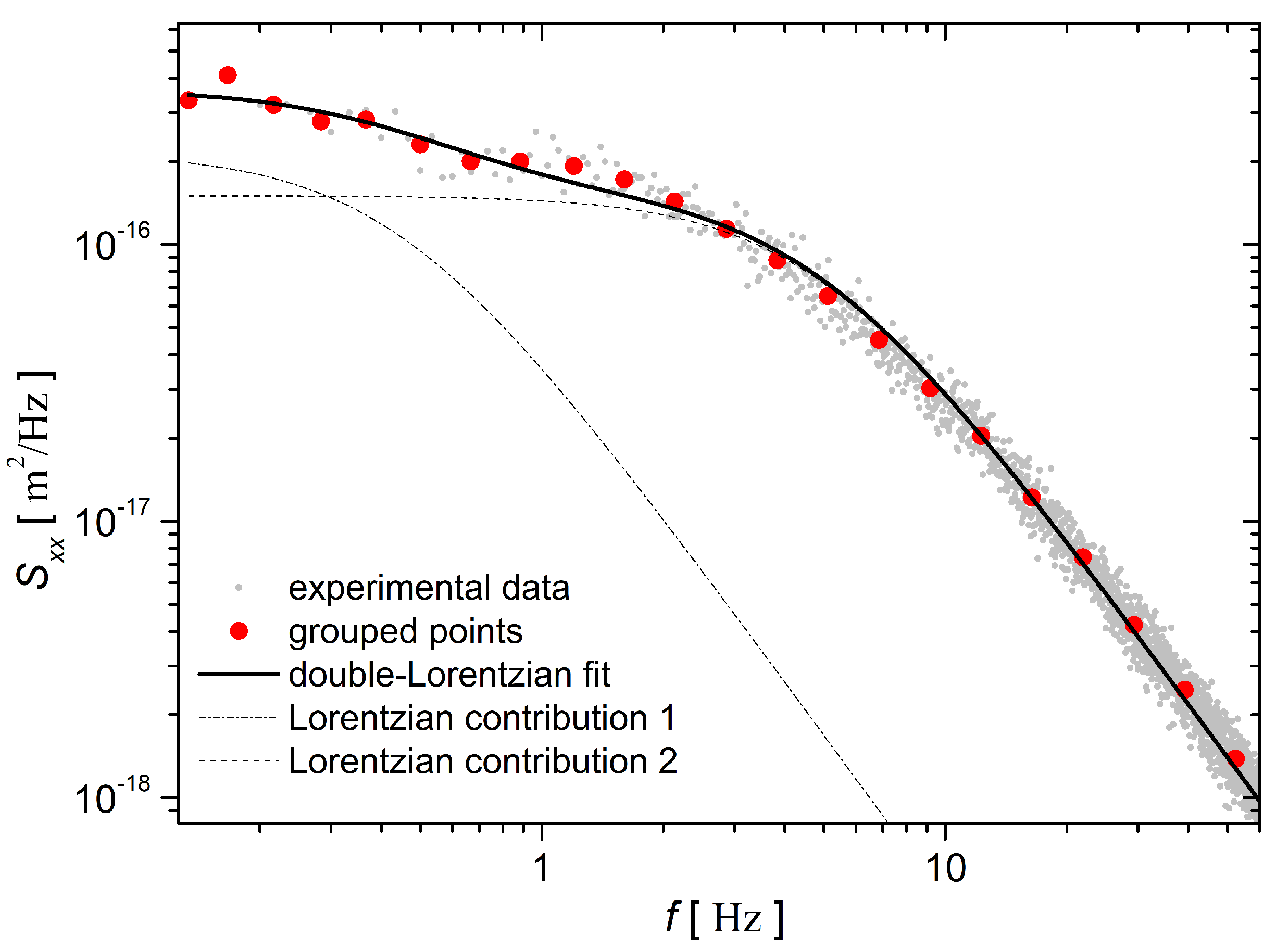
4.7. Experimental Results and Their Regression

After the successful implementation of the experiment, we obtained data representing the observed dynamics $x\left(t\right)$, which we have then transformed into corresponding Fourier images. The aim was to obtain an experimental power spectrum density ${\{S_{xx,j}^{\mathrm{ex}}\}}_{j=1}^{N^{\mathrm{ex}}}$ for the system of $N^{\mathrm{ex}}$ frequencies ${\left\{f_j\right\}}_{j=1}^{N^{\mathrm{ex}}}$ (see Figure 3). Some of the evaluations have been performed according to the work of [19]. Preprocessing with grouping of the adjacent experimental spectral points is a necessary methodological peculiarity. Frequency and spectrum groupings with eight points over the frequency decade were introduced. The effectiveness with which the representative grouping frequencies were allocated was evaluated. Naturally, the grouping process affects not only the locations of representative frequencies, but also the statistics of spectral points, potentially increasing the regression’s feasibility. The optimization of parametric combinations is made possible by data knowledge. Let us formally encapsulate the unknown model parameters in a single symbol $\mathsf{Par}$, resulting in the parameterized form of the double Lorentzian model $S_{xx}(f_j,\mathsf{Par})$ (see Equation (29)). In addition to identifying the optimum, we will focus on estimating errors for various components of $\mathsf{Par}$.

The problem-specific emphasis is on the asymptotic behavior of the spectrum. Despite the fact that the density of the power spectrum decreases as $\sim f^{-2}$, the high frequency domain must be properly included in the regression due to its physical significance. Hence, a weighted regression of the squares of $S_{xx}(f_j,\mathsf{Par})-S_{xx,j}^{\mathrm{ex}}$ deviations has been implemented. The preference can be defined as the minimization of the objective function

$$\mathsf{Obj}\_\mathsf{F}\left(\mathsf{Par}\right)\equiv \sum _{j=1}^{N^{\mathrm{ex}}}{\left[\frac{S_{xx}(f_j,\mathsf{Par})-S_{xx,j}^{\mathrm{ex}}}{S_{xx,j}^{\mathrm{ex}}}\right]}^2.$$

(47)

Here, the parameters and their combinations appear to be formally merged into the vector

$$\mathsf{Par}\equiv \left(f_{\mathrm{C}1},f_{\mathrm{C}2},\frac{K_{\mathrm{A}}}{4{\pi }^2},\frac{k_{\mathrm{B}}T}{2{\pi }^2\gamma }\right).$$

(48)

This is subject to optimization. We used the standard global function optimizer, which was built on the concept of the [26] work with the implementation (scypy.optimize.curve_fit(…)) to the SciPy library [27]. The regression corresponding to $\mathsf{Obj}\_\mathsf{F}$ provides the corner frequencies

$$f_{\mathrm{C}1}=\left(0.443\pm 0.093\right)\left(\mathrm{Hz}\right),f_{\mathrm{C}2}=\left(4.82\pm 0.23\right)\left(\mathrm{Hz}\right).$$

(49)

Along with them

$$\frac{K_{\mathrm{A}}}{4{\pi }^2}=\left(0.47\pm 0.19\right)\left({\mathrm{Hz}}^2\right).$$

(50)

Finally, there is also fixed corresponding parametric combination

$$\frac{k_{\mathrm{B}}T}{2{\pi }^2\gamma }=\left(3.53\pm 0.13\right)\times {10}^{-15}\left({\mathrm{m}}^2\mathrm{Hz}\right),$$

(51)

which represents the constant factor in $S_{xx}(f,\mathsf{Par})$ as defined by Equation (29). The regression outcomes are depicted in Figure 3.

Now there is a standard way to find out the autocorrelation function (see Equation (37)) via the respective parameters

$$\begin{array}{ccc}\hfill \frac{{\mathcal{R}}_0}{\pi }& =& \frac{\left(\frac{k_{\mathrm{B}}T}{2{\pi }^2\gamma }\right)}{f_{\mathrm{C}2}^2-f_{\mathrm{C}1}^2}=1.532\times {10}^{-16}({\mathrm{m}}^2/\mathrm{Hz}),\hfill \\ & & \hfill \\ \hfill {\mathcal{R}}_1& =& 0.623\left(\mathrm{Hz}\right),{\mathcal{R}}_2=4.723\left(\mathrm{Hz}\right).\hfill \end{array}$$

(52)

A posteriori evaluation methodology following the regression results provides an implication for the values of the regression-related spectral moments

$$\begin{array}{ccc}\hfill {\mathcal{M}}_{\mathrm{Sxx}}^{\mathrm{rr}}(0,f_{\mathrm{C}1})& =& 1.414\times {10}^{-16}\left({\mathrm{m}}^2\right),\hfill \\ \hfill {\mathcal{M}}_{\mathrm{Sxx}}^{\mathrm{rr}}(f_{\mathrm{C}1},f_{\mathrm{C}2})& =& 5.682\times {10}^{-16}\left({\mathrm{m}}^2\right),\hfill \\ \hfill {\mathcal{M}}_{\mathrm{Sxx}}^{\mathrm{rr}}(f_{\mathrm{C}2},\infty )& =& 5.772\times {10}^{-16}\left({\mathrm{m}}^2\right).\hfill \end{array}$$

(53)

We see that the sum of the moments $1.286\times {10}^{-15}$$\left({\mathrm{m}}^2\right)$ equals $({\mathcal{R}}_0/2)$ $({\mathcal{R}}_1+{\mathcal{R}}_2)$, as predicted.

Adjusting the integration boundaries can be important for the design of some alternative test moments. The premise of the adjustment is that these variants should be more closely linked to the measurement process, conditioned by the need to avoid spectral distortions known as “aliasing” and “motion blur”. The effects occur due to too superficial and insufficient sampling of the signal $x\left(t\right)$ captured by the camera. This means that the calculations must focus on bands with frequencies less than $f_{\mathrm{upp}}$, which in our case was set to around a quarter of the Nyquist frequency. The lower limit value $f_{\mathrm{low}}$ prevents the use of extremely low frequencies. Respecting the lower limit suppresses distortions caused by the apparatus background noise. Numerically, the boundaries we introduce are $f_{\mathrm{low}}=0.1333$ $\left[\mathrm{Hz}\right]$ and $f_{\mathrm{upp}}=59.97$ $\left[\mathrm{Hz}\right]$. The following three moments

$$\begin{array}{ccc}\hfill {\mathcal{M}}_{\mathrm{Sxx}}^{\mathrm{ex}}(f_{\mathrm{low}},f_{\mathrm{C}1})& =& 0.924\times {10}^{-16}\left({\mathrm{m}}^2\right),\hfill \\ \hfill {\mathcal{M}}_{\mathrm{Sxx}}^{\mathrm{ex}}(f_{\mathrm{C}1},f_{\mathrm{C}2})& =& 5.687\times {10}^{-16}\left({\mathrm{m}}^2\right),\hfill \\ \hfill {\mathcal{M}}_{\mathrm{Sxx}}^{\mathrm{ex}}(f_{\mathrm{C}2},f_{\mathrm{upp}})& =& 4.952\times {10}^{-16}\left({\mathrm{m}}^2\right)\hfill \end{array}$$

(54)

were created to express the properties of the experimental data set, which was achieved by partly reducing the impact of the regression results. Here we see that Simpson’s integration quadrature based on uniform data sampling (without grouping) also provides us with variants of spectral moments. However, even when using numerical integration, we must be careful if we subsequently perform comparisons and interpretations. The reason is that certain integrals approximated by a suitable summation can become dependent on the previous regression only by their integration boundaries when these are linked to regression parameters ($f_{\mathrm{C}1}$ and $f_{\mathrm{C}2}$). Independence from regression can be achieved using descriptive spectrum characteristics (analogous to descriptive statistics). This means using characteristic frequencies in the role of integration boundaries. Then the results of the calculation are generalized spectral averages. The fact that we do not present more moment variants here is mainly related to the focus of this work.

When comparing the Equations (53) and (54), we see that only the central moments for the $[f_{\mathrm{C}1}$, $f_{\mathrm{C}2}]$ band are close enough to each other, which means that ${\mathcal{M}}_{\mathrm{Sxx}}^{\mathrm{rr}}(0,f_{\mathrm{C}1})$ and ${\mathcal{M}}_{\mathrm{Sxx}}^{\mathrm{rr}}(f_{\mathrm{C}2},\infty )$ are not sufficient approximations of ${\mathcal{M}}_{\mathrm{Sxx}}^{\mathrm{ex}}(f_{\mathrm{low}},f_{\mathrm{C}1})$ and ${\mathcal{M}}_{\mathrm{Sxx}}^{\mathrm{ex}}(f_{\mathrm{C}2},f_{\mathrm{upp}})$, respectively. Results show that in the case of regression-related moments, there is only a slight and negligible rise in moments compared to the use of Simpson’s rule

$$\begin{array}{ccc}\hfill \underline{\sim 1.2\%\mathrm{increase}}:& & \hfill \\ \hfill {\mathcal{M}}_{\mathrm{Sxx}}^{\mathrm{rr}}(0,f_{\mathrm{C}1})-{\mathcal{M}}_{\mathrm{Sxx}}^{\mathrm{rr}}(0,f_{\mathrm{low}})& =& 0.935\times {10}^{-16}\left({\mathrm{m}}^2\right)\hfill \\ & \gtrsim & {\mathcal{M}}_{\mathrm{Sxx}}^{\mathrm{ex}}(f_{\mathrm{low}},f_{\mathrm{C}1}),\hfill \\ & & \hfill \\ \hfill \underline{\sim 4.6\%\mathrm{increase}}:& & \hfill \\ \hfill {\mathcal{M}}_{\mathrm{Sxx}}^{\mathrm{rr}}(f_{\mathrm{C}2},\infty )-{\mathcal{M}}_{\mathrm{Sxx}}^{\mathrm{rr}}(f_{\mathrm{upp}},\infty )& =& 5.184\times {10}^{-16}\left({\mathrm{m}}^2\right)\hfill \\ & \gtrsim & {\mathcal{M}}_{\mathrm{Sxx}}^{\mathrm{ex}}(f_{\mathrm{C}2},f_{\mathrm{upp}}).\hfill \end{array}$$

(55)

5. Discussion

Two kinds of spectral moments (${\mathcal{M}}_{\mathrm{Sxx}}^{\mathrm{rr}}(.)$ and ${\mathcal{M}}_{\mathrm{SSx}}^{\mathrm{ex}}(.))$ were designed, calculated and compared for the experimental input data given. We have shown by analysis that subsequent regression-related and the numerical integration outputs can be globally or locally compared and evaluated. This would have an effect on the choice of the overall regression process or model, thereby affecting at least one of them.

The studied model is based on the assumption that a pair of different corner frequencies is needed to describe the spectrum. Consider a situation that, under certain parametric conditions, only a small gap between $f_{\mathrm{C}1}$ and $f_{\mathrm{C}2}$ is observable. Alternatively, one of the two spectrum amplitudes before the terms $1/(f_{\mathrm{C}1}^2+f^2)$, $1/(f_{\mathrm{C}2}^2+f^2)$ may be negligible (see Equation (29)). All these cases lead to a special limit of the single Lorentz power spectral density.

It should be noted that we did not study beyond the level of a few phenomenological parameters provided in $\mathsf{Par}$ on purpose. This is related to the reasons for which the correct determination of the four constants $k_1,k_2,\gamma ,\delta$ is part of a wider methodological issue that demands the use of several independent observations. The nanowire material properties, rather than the model’s less universal parameters, will likely be the focus of our future research.

6. Conclusions

Nanowires prepared by TPP-DLW from Ormocomp possess viscoelastic material properties. This viscoelasticity determines the mechanical behavior of microstructures comprising such nanowires.

The bending recovery motion of cantilevered nanowire systems equipped with a microbead at the free end and immersed in Newtonian liquids was studied previously [25]. The same microstructures, in isolation, exhibit significant thermal fluctuations. In this work, the previous mechanical model was extended with stochastic forces to explain the power spectral density and autocorrelation function of the microstructure thermal fluctuations. In principle, the Brownian fluctuations of cantilevered nanowires can be utilized for micron-scale viscosity measurements. Our results pave the way for a quantitative analysis of such micro-viscometer systems.

The calculation of the correlation functions of the characteristic coordinate was carried out in the frequency domain by introducing symmetric forms for the corresponding coefficients. The implications of the calculation concern the steady state, which can be alternatively characterized by the spectral power density. An interesting aspect of our approach is that the weighted regression results for the spectra have been validated using the spectral moment system.

Theoretical considerations confirmed the double-Lorentzian power density spectrum and the doubly-exponential autocorrelation function. As we have shown by a special implementation of weighted regression, reasonable agreement with our experimental observations was obtained for the spectrum. Simultaneous weighted regression of multiple functions, including autocorrelation, is reserved for further empirically oriented work.

It is concluded that the source of thermal fluctuations is related both to energy dissipation inside the photopolymer material and the surrounding liquid. In this partial dissipation problem, we have shown that the equipartition theorem allows us to correctly parameterize random forces. Furthermore, we believe that the stochastic mechanical model we present has the potential to be used for further analysis and prediction of characteristics for similar nanowire-based systems.

References

1. Kappler, E. Versuche zur Messung der Avogadro-Loschmidtschen Zahl aus der Brownschen Bewegung einer Drehwaage. Ann. Der Phys. 1931, 403, 233–256. [Google Scholar] [CrossRef]
2. Sader, J.E. Frequency response of cantilever beams immersed in viscous fluids with applications to the atomic force microscope. J. Appl. Phys. 1998, 84. [Google Scholar] [CrossRef] [Green Version]
3. Boskovic, S.; Chon, J.W.M.; Mulvaney, P.; Sader, J.E. Rheological measurements using microcantilevers. J. Rheol. 2002, 46, 891–899. [Google Scholar] [CrossRef]
4. Kara, V.; Sohn, Y.I.; Atikian, H.; Yakhot, V.; Lončar, M.; Ekinci, K.L. Nanofluidics of Single-Crystal Diamond Nanomechanical Resonators. Nano Lett. 2015, 15, 8070–8076. [Google Scholar] [CrossRef]
5. Miller, J.M.L.; Ansari, A.; Heinz, D.B.; Chen, Y.H.; Flader, I.B.; Shin, D.D.; Villanueva, L.G.; Kenny, T.W. Effective quality factor tuning mechanisms in micromechanical resonators. Appl. Phys. Rev. 2018, 5, 041307. [Google Scholar] [CrossRef]
6. Paul, M.R.; Clark, M.T.; Cross, M.C. The stochastic dynamics of micron and nanoscale elastic cantilevers in fluid: Fluctuations from dissipation. Nanotechnology 2006, 17, 4502. [Google Scholar] [CrossRef]
7. Meyhöfer, E.; Howard, J. The force generated by a single kinesin molecule against an elastic load. Proc. Natl. Acad. Sci. USA 1995, 92, 574–578. [Google Scholar] [CrossRef] [Green Version]
8. Viani, M.B.; Schäffer, T.E.; Chand, A.; Rief, M.; Gaub, H.E.; Hansma, P.K. Small cantilevers for force spectroscopy of single molecules. J. Appl. Phys. 1999, 86, 2258–2262. [Google Scholar] [CrossRef]
9. Fan, H.F.; Ma, C.H.; Jayaram, M. Single-Molecule Tethered Particle Motion: Stepwise Analyses of Site-Specific DNA Recombination. Micromachines 2018, 9, 216. [Google Scholar] [CrossRef] [Green Version]
10. Kovari, D.T.; Yan, Y.; Finzi, L.; Dunlap, D. Tethered Particle Motion: An Easy Technique for Probing DNA Topology and Interactions with Transcription Factors. Methods Mol. Biol. 2018, 1665, 317–340. [Google Scholar] [CrossRef]
11. Manghi, M.; Destainville, N.; Brunet, A. Statistical physics and mesoscopic modeling to interpret tethered particle motion experiments. Methods 2019, 169, 57–68. [Google Scholar] [CrossRef] [Green Version]
12. Huang, Y.; Flores, F.; Jaime, G.; Li, Y.; Wang, W.; Wang, D.; Goldberg, N.; Zheng, J.; Yu, M.; Lu, M.; et al. A Chip-Scale Oscillation-Mode Optomechanical Inertial Sensor Near the Thermodynamical Limits. Laser Photonics Rev. 2020, 14, 1800329. [Google Scholar] [CrossRef] [Green Version]
13. Hines, A.; Richardson, L.; Wisniewski, H.; Guzman, F. Optomechanical inertial sensors. Appl. Opt. 2020, 59, G167–G174. [Google Scholar] [CrossRef]
14. Geraci, A.; Bradley, C.; Gao, D.; Weinstein, J.; Derevianko, A. Searching for Ultralight Dark Matter with Optical Cavities. Phys. Rev. Lett. 2019, 123, 031304. [Google Scholar] [CrossRef] [PubMed] [Green Version]
15. Catano-Lopez, S.B.; Santiago-Condori, J.G.; Edamatsu, K.; Matsumoto, N. High-Q Milligram-Scale Monolithic Pendulum for Quantum-Limited Gravity Measurements. Phys. Rev. Lett. 2020, 124, 221102. [Google Scholar] [CrossRef]
16. Sharifi, S.; Banadaki, Y.; Cullen, T.; Veronis, G.; Dowling, J.; Corbitt, T. Design of microresonators to minimize thermal noise below the standard quantum limit. Rev. Sci. Instruments 2020, 91, 054504. [Google Scholar] [CrossRef] [PubMed]
17. Saulson, P.R. Thermal noise in mechanical experiments. Phys. Rev. D 1990, 42, 2437–2445. [Google Scholar] [CrossRef]
18. Howard, J. Mechanics of Motor Proteins and the Cytoskeleton; Sinauer Associates: Sunderland, MA, USA, 2001; Volume 55. [Google Scholar] [CrossRef]
19. Berg-Sorensen, K.; Flyvbjerg, H. Power spectrum analysis for optical tweezers. Rev. Sci. Instruments 2004, 75, 594–612. [Google Scholar] [CrossRef] [Green Version]
20. Lukić, B.; Jeney, S.; Sviben, Ž.; Kulik, A.J.; Florin, E.L.; Forró, L. Motion of a colloidal particle in an optical trap. Phys. Rev. E 2007, 76, 011112. [Google Scholar] [CrossRef] [PubMed] [Green Version]
21. Malinauskas, M.; Farsari, M.; Piskarskas, A.; Juodkazis, S. Ultrafast laser nanostructuring of photopolymers: A decade of advances. Phys. Rep. Rev. Sect. Phys. Lett. 2013, 533, 1–31. [Google Scholar] [CrossRef]
22. LaFratta, C.N.; Fourkas, J.T.; Baldacchini, T.; Farrer, R.A. Multiphoton fabrication. Angew. Chem. Int. Ed. 2007, 46, 6238–6258. [Google Scholar] [CrossRef]
23. Nakanishi, S.; Shoji, S.; Kawata, S.; Sun, H.B. Giant elasticity of photopolymer nanowires. Appl. Phys. Lett. 2007, 91, 063112. [Google Scholar] [CrossRef]
24. Cayll, D.R.; Ladner, I.S.; Cho, J.H.; Saha, S.K.; Cullinan, M.A. A MEMS dynamic mechanical analyzer for in situ viscoelastic characterization of 3D printed nanostructures. J. Micromech. Microeng. Struct. Devices Syst. 2020, 30, 075008. [Google Scholar] [CrossRef]
25. Kubacková, J.; Iváni, G.T.; Kažiková, V.; Strejčková, A.; Hovan, A.; Žoldák, G.; Vizsnyiczai, G.; Kelemen, L.; Tomori, Z.; Bánó, G. Bending dynamics of viscoelastic photopolymer nanowires. Appl. Phys. Lett. 2020, 117, 013701. [Google Scholar] [CrossRef]
26. Burden, R.; Faires, J. Numerical Analysis, 4th ed.; The Prindle, Weber and Schmidt Series in Mathematics; PWS-Kent Publishing Company: Boston, FL, USA, 1989. [Google Scholar]
27. Virtanen, P.; Gommers, R.; Oliphant, T.E.; Haberland, M.; Reddy, T.; Cournapeau, D.; Burovski, E.; Peterson, P.; Weckesser, W.; Bright, J.; et al. SciPy 1.0: Fundamental Algorithms for Scientific Computing in Python. Nat. Methods 2020, 17, 261–272. [Google Scholar] [CrossRef] [PubMed] [Green Version]
Figure 1. The main steps from sample preparation to measurement. (a) Light-sensitive (photoresist) material exposed to the laser beam. Single photon (left part, in blue) and two-photon (right part, in red) polymerization is depicted separately. (The exceptional spatial resolution can be reached by the two-photon process. The polymerized material is indicated in gray.) (b) The illumination used to produce three-dimensional design in the photoresist volume employing TPP-DLW. (c) Setup for motion detection and data production. The application of a CMOS image sensor, which provides encoded light information about position x ( t ) that can be converted into digital data records by particle tracking algorithms. (d) A closer look at the mechanics of Brownian fluctuations under anchoring conditions. The studied fluctuations in the horizontal plane are indicated by the arrows.
Mathematics 09 01748 g001
Figure 2. The schematic depiction of the linear mechanical model for the microbead motion. Arms A and B represent the nanowire and the hydrodynamic damping by the surrounding medium, respectively. The internal characteristics x 1 , x 2 are related to the total observable parameter x.
Mathematics 09 01748 g002
Figure 3. Power spectral density of microsphere fluctuations. The solid line belongs to the model according to Equation (29). The fit was set after optimization of Obj _ F ( Par ) . Two Lorentzian contributions spanning the entire spectrum are also shown.
Mathematics 09 01748 g003
Publisher’s Note: MDPI stays neutral with regard to jurisdictional claims in published maps and institutional affiliations.