
An Extension of Explicit Coupling for Fluid–Structure Interaction Problems


Abstract
:1. Introduction
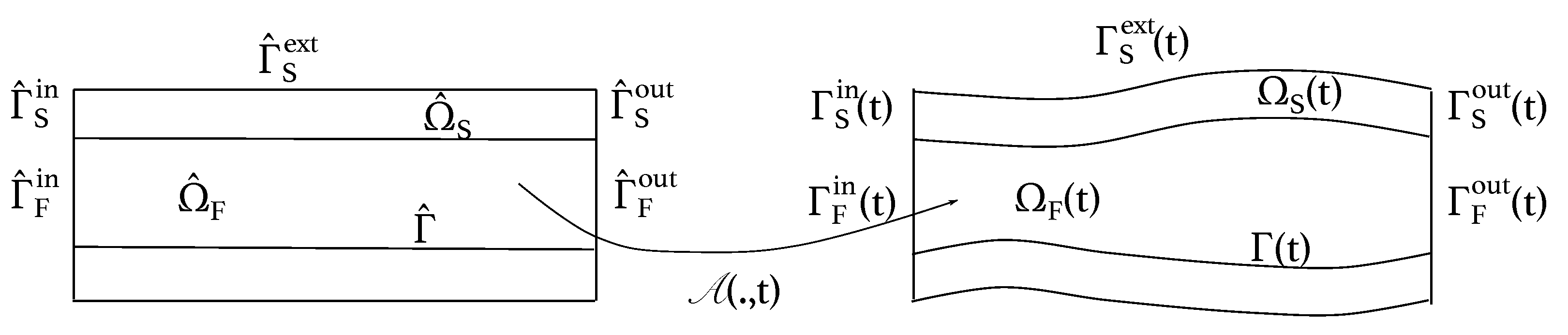
2. Problem Description
3. Numerical Method
| Algorithm 1 Given in , and in , for all , compute the following steps: |
Structure sub-problem: Find and such that
Fluid sub-problem: Find and such that
|
| Algorithm 2 Given in , and in , we first need to compute in , and in . A monolithic method could be used. Then, for all , compute the following steps: |
Structure sub-problem: Find and such that
Fluid sub-problem: Find and such that
|
3.1. Stability Analysis
3.2. Extensions to the Moving Domain FSI
4. Numerical Results
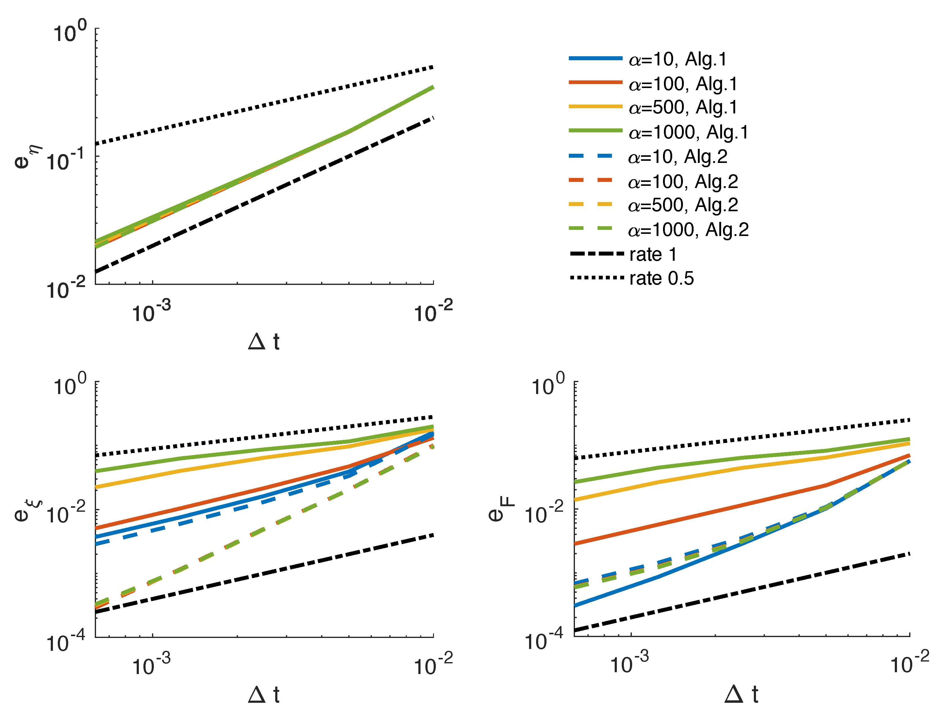
4.1. Example 1
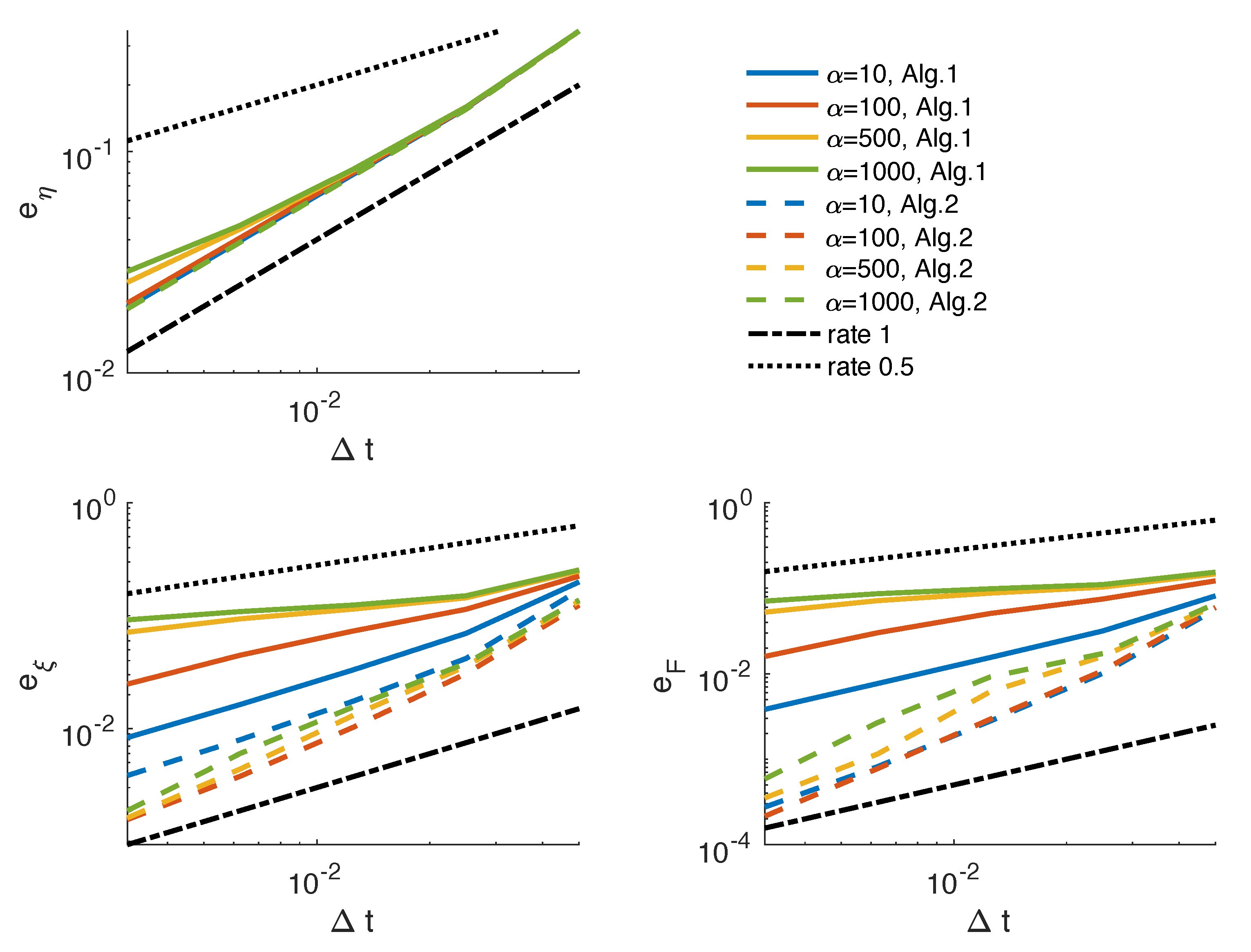
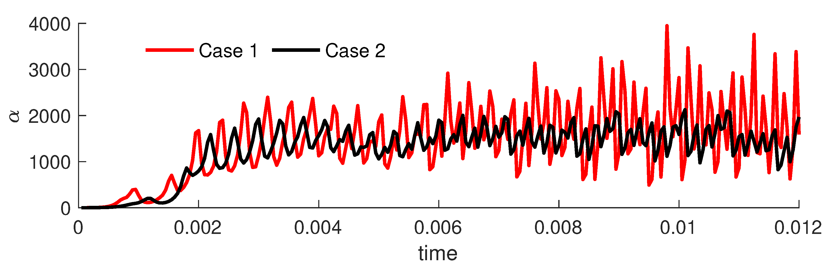
4.2. Example 2
| Algorithm 3 Given in , and in , we first need to compute in , and in . A monolithic method could be used. Then, for all , compute the following steps: |
Structure sub-problem: Find and such that
Geometry sub-problem: Find such that
Compute as . Fluid sub-problem: Find and such that
|
5. Conclusions
Funding
Data Availability Statement
Conflicts of Interest
Abbreviations
| FSI | Fluid–structure interaction |
Appendix A. Inequalities Used in the Stability Analysis
References
- Hou, G.; Wang, J.; Layton, A. Numerical methods for fluid-structure interaction: A review. Commun. Comput. Phys. 2012, 12, 337–377. [Google Scholar] [CrossRef]
- Gee, M.; Küttler, U.; Wall, W. Truly monolithic algebraic multigrid for fluid–structure interaction. Int. J. Numer. Methods Eng. 2011, 85, 987–1016. [Google Scholar] [CrossRef]
- Badia, S.; Quaini, A.; Quarteroni, A. Modular vs. non-modular preconditioners for fluid–structure systems with large added-mass effect. Comput. Methods Appl. Mech. Eng. 2008, 197, 4216–4232. [Google Scholar] [CrossRef] [Green Version]
- Heil, M.; Hazel, A.; Boyle, J. Solvers for large-displacement fluid–structure interaction problems: Segregated versus monolithic approaches. Comput. Mech. 2008, 43, 91–101. [Google Scholar] [CrossRef]
- Burman, E.; Durst, R.; Fernández, M.; Guzmán, J. Fully discrete loosely coupled Robin-Robin scheme for incompressible fluid-structure interaction: Stability and error analysis. arXiv 2020, arXiv:2007.03846. [Google Scholar]
- Burman, E.; Fernández, M. Stabilization of explicit coupling in fluid-structure interaction involving fluid incompressibility. Comput. Methods Appl. Mech. Eng. 2009, 198, 766–784. [Google Scholar] [CrossRef] [Green Version]
- Fernández, M.; Mullaert, J.; Vidrascu, M. Generalized Robin–Neumann explicit coupling schemes for incompressible fluid-structure interaction: Stability analysis and numerics. Int. J. Numer. Methods Eng. 2015, 101, 199–229. [Google Scholar] [CrossRef] [Green Version]
- Bukac, M.; Muha, B. Stability and Convergence Analysis of the Extensions of the Kinematically Coupled Scheme for the Fluid-Structure Interaction. SIAM J. Numer. Anal. 2016, 54, 3032–3061. [Google Scholar] [CrossRef]
- Seboldt, A.; Bukač, M. A non-iterative domain decomposition method for the interaction between a fluid and a thick structure. Numer. Methods Partial. Differ. Equations 2021, 37, 2803–2832. [Google Scholar] [CrossRef]
- Oyekole, O.; Trenchea, C.; Bukac, M. A Second-Order in Time Approximation of Fluid-Structure Interaction Problem. SIAM J. Numer. Anal. 2018, 56, 590–613. [Google Scholar] [CrossRef]
- Fernández, M. Incremental displacement-correction schemes for incompressible fluid-structure interaction: Stability and convergence analysis. Numer. Math. 2012, 123, 210–265. [Google Scholar] [CrossRef] [Green Version]
- Lukáčová-Medvid’ová, M.; Rusnáková, G.; Hundertmark-Zaušková, A. Kinematic splitting algorithm for fluid–structure interaction in hemodynamics. Comput. Methods Appl. Mech. Eng. 2013, 265, 83–106. [Google Scholar] [CrossRef]
- Langer, U.; Yang, H. 5. Recent development of robust monolithic fluid-structure interaction solvers. In Fluid-Structure Interaction; De Gruyter: Berlin, Germany, 2017; pp. 169–192. [Google Scholar]
- Nobile, F.; Vergara, C. An effective fluid-structure interaction formulation for vascular dynamics by generalized Robin conditions. SIAM J. Sci. Comput. 2008, 30, 731–763. [Google Scholar] [CrossRef]
- Badia, S.; Nobile, F.; Vergara, C. Robin-Robin preconditioned Krylov methods for fluid-structure interaction problems. Comput. Methods Appl. Mech. Eng. 2009, 198, 2768–2784. [Google Scholar] [CrossRef] [Green Version]
- Badia, S.; Nobile, F.; Vergara, C. Fluid-structure partitioned procedures based on Robin transmission conditions. J. Comput. Phys. 2008, 227, 7027–7051. [Google Scholar] [CrossRef]
- Gerardo-Giorda, L.; Nobile, F.; Vergara, C. Analysis and Optimization of Robin-Robin Partitioned Procedures in Fluid-Structure Interaction Problems. SIAM J. Numer. Anal. 2010, 48, 2091–2116. [Google Scholar] [CrossRef] [Green Version]
- Degroote, J. On the similarity between Dirichlet–Neumann with interface artificial compressibility and Robin–Neumann schemes for the solution of fluid-structure interaction problems. J. Comput. Phys. 2011, 230, 6399–6403. [Google Scholar] [CrossRef] [Green Version]
- Baek, H.; Karniadakis, G. A convergence study of a new partitioned fluid–structure interaction algorithm based on fictitious mass and damping. J. Comput. Phys. 2012, 231, 629–652. [Google Scholar] [CrossRef]
- Yu, Y.; Baek, H.; Karniadakis, G. Generalized fictitious methods for fluid–structure interactions: Analysis and simulations. J. Comput. Phys. 2013, 245, 317–346. [Google Scholar] [CrossRef]
- Burman, E.; Fernández, M. An unfitted Nitsche method for incompressible fluid-structure interaction using overlapping meshes. Comput. Methods Appl. Mech. Eng. 2014, 279, 497–514. [Google Scholar] [CrossRef]
- Banks, J.; Henshaw, W.; Schwendeman, D. An analysis of a new stable partitioned algorithm for FSI problems. Part I: Incompressible flow and elastic solids. J. Comput. Phys. 2014, 269, 108–137. [Google Scholar] [CrossRef]
- Serino, D.; Banks, J.; Henshaw, W.; Schwendeman, D. A stable added-mass partitioned (AMP) algorithm for elastic solids and incompressible flow: Model problem analysis. SIAM J. Sci. Comput. 2019, 41, A2464–A2484. [Google Scholar] [CrossRef]
- Bukač, M.; Čanić, S.; Glowinski, R.; Muha, B.; Quaini, A. A modular, operator-splitting scheme for fluid–structure interaction problems with thick structures. Int. J. Numer. Methods Fluids 2014, 74, 577–604. [Google Scholar] [CrossRef] [Green Version]
- Burman, E.; Fernández, M.A. Explicit strategies for incompressible fluid-structure interaction problems: Nitsche type mortaring versus Robin–Robin coupling. Int. J. Numer. Methods Eng. 2014, 97, 739–758. [Google Scholar] [CrossRef]
- Burman, E.; Durst, R.; Guzman, J. Stability and error analysis of a splitting method using Robin-Robin coupling applied to a fluid-structure interaction problem. arXiv 2019, arXiv:1911.06760. [Google Scholar]
- Hughes, T.; Liu, W.; Zimmermann, T. Lagrangian-Eulerian finite element formulation for incompressible viscous flows. Comput. Methods Appl. Mech. Eng. 1981, 29, 329–349. [Google Scholar] [CrossRef]
- Donea, J. Arbitrary Lagrangian-Eulerian finite element methods. In Computational Methods for Transient Analysis; North-Holland: Amsterdam, The Netherlands, 1983; pp. 473–516. [Google Scholar]
- Nobile, F. Numerical Approximation of Fluid-Structure Interaction Problems with Application to Haemodynamics. Ph.D. Thesis, EPFL, Lausanne, Switzerland, 2001. [Google Scholar]
- Langer, U.; Yang, H. Numerical simulation of fluid–structure interaction problems with hyperelastic models: A monolithic approach. Math. Comput. Simul. 2018, 145, 186–208. [Google Scholar] [CrossRef] [Green Version]
- Bukač, M.; Čanić, S.; Muha, B. A partitioned scheme for fluid–composite structure interaction problems. J. Comput. Phys. 2015, 281, 493–517. [Google Scholar] [CrossRef] [Green Version]
- Formaggia, L.; Quarteroni, A.; Veneziani, A. Cardiovascular Mathematics: Modeling and Simulation of the Circulatory System; Springer Science & Business Media: Berlin/Heidelberg, Germany, 2010; Volume 1. [Google Scholar]
- Girault, V.; Raviart, P.A. Finite Element Methods for Navier–Stokes Equations: Theory and Algorithms; Springer Science & Business Media: Berlin/Heidelberg, Germany, 2012; Volume 5. [Google Scholar]


| 10 | 100 | 500 | 1000 | 10 | 100 | 500 | 1000 | |
|---|---|---|---|---|---|---|---|---|
| Algorithm 1 | ||||||||
| - | - | - | - | - | - | - | - | |
| 2.04 | 1.49 | 0.89 | 0.78 | 2.48 | 1.57 | 0.74 | 0.61 | |
| 1.27 | 1.12 | 0.58 | 0.41 | 1.84 | 1.03 | 0.54 | 0.37 | |
| 1.11 | 1.06 | 0.69 | 0.47 | 1.72 | 1.01 | 0.75 | 0.51 | |
| 1.02 | 1.03 | 0.85 | 0.66 | 1.5 | 1.01 | 0.92 | 0.75 | |
| Algorithm 2 | ||||||||
| - | - | - | - | - | - | - | - | |
| 2.18 | 2.30 | 2.26 | 2.24 | 2.4 | 2.43 | 2.44 | 2.44 | |
| 1.34 | 2.02 | 2.05 | 2.03 | 1.62 | 1.72 | 1.74 | 1.78 | |
| 1.15 | 2.12 | 2.13 | 2.13 | 1.28 | 1.33 | 1.33 | 1.34 | |
| 1.05 | 1.99 | 1.81 | 1.79 | 1.08 | 1.07 | 1.06 | 1.05 |
| 10 | 100 | 500 | 1000 | 10 | 100 | 500 | 1000 | |
|---|---|---|---|---|---|---|---|---|
| Algorithm 1 | ||||||||
| - | - | - | - | - | - | - | - | |
| 1.51 | 0.97 | 0. 79 | 0.76 | 1.36 | 0.71 | 0.51 | 0.48 | |
| 1.08 | 0.64 | 0.33 | 0.27 | 1.03 | 0.56 | 0.23 | 0.16 | |
| 1.02 | 0.71 | 0.29 | 0.19 | 1.01 | 0.75 | 0.29 | 0.19 | |
| 0.97 | 0.85 | 0.39 | 0.24 | 1.0 | 0.92 | 0.45 | 0.29 | |
| Algorithm 2 | ||||||||
| - | - | - | - | - | - | - | - | |
| 2.01 | 2.01 | 1.91 | 1.86 | 2.48 | 2.45 | 1.98 | 1.94 | |
| 1.26 | 1.58 | 1.45 | 1.28 | 1.86 | 1.89 | 1.37 | 0.91 | |
| 1.13 | 1.44 | 1.58 | 1.37 | 1.77 | 1.92 | 2.42 | 1.78 | |
| 1.05 | 1.28 | 1.44 | 1.69 | 1.57 | 1.85 | 1.71 | 2.18 |
| Parameters | Values | Parameters | Values |
|---|---|---|---|
| Fluid density (g/cm) | 1 | Dyn. viscosity (poise) | |
| Wall density (g/cm) | Spring coeff. (dynes/cm) | ||
| Shear mod. (dyne/cm) | Lamé’s 1st par. (dyne/cm) |
Publisher’s Note: MDPI stays neutral with regard to jurisdictional claims in published maps and institutional affiliations. |
© 2021 by the author. Licensee MDPI, Basel, Switzerland. This article is an open access article distributed under the terms and conditions of the Creative Commons Attribution (CC BY) license (https://creativecommons.org/licenses/by/4.0/).
Share and Cite
Bukač, M. An Extension of Explicit Coupling for Fluid–Structure Interaction Problems. Mathematics 2021, 9, 1747. https://doi.org/10.3390/math9151747
Bukač M. An Extension of Explicit Coupling for Fluid–Structure Interaction Problems. Mathematics. 2021; 9(15):1747. https://doi.org/10.3390/math9151747
Chicago/Turabian StyleBukač, Martina. 2021. "An Extension of Explicit Coupling for Fluid–Structure Interaction Problems" Mathematics 9, no. 15: 1747. https://doi.org/10.3390/math9151747
APA StyleBukač, M. (2021). An Extension of Explicit Coupling for Fluid–Structure Interaction Problems. Mathematics, 9(15), 1747. https://doi.org/10.3390/math9151747