Abstract
The spread of the SARS-CoV-2 modeling is a challenging problem because of its complex nature and lack of information regarding certain aspects. In this paper, we explore a Digital Twin approach to model the pandemic situation in Catalonia. The Digital Twin is composed of three different dynamic models used to perform the validations by a Model Comparison approach. We detail how we use this approach to obtain knowledge regarding the effects of the nonpharmaceutical interventions and the problems we faced during the modeling process. We use Specification and Description Language (SDL) to represent the compartmental forecasting model for the SARS-CoV-2. Its graphical notation simplifies the different specialists’ understanding of the model hypotheses, which must be validated continuously following a Solution Validation approach. This model allows the successful forecasting of different scenarios for Catalonia. We present some formalization details, discuss the validation process and present some results obtained from the validation model discussion, which becomes a digital twin of the pandemic in Catalonia.
1. Introduction
Computer simulations to forecast the infections, based on the Susceptible, Exposed, Infected and Recovered and Death (SEIRD) models are common since its preliminary inception in 1930 [1] These models can be used to represent a pandemic situation and to forecast the new cases due to SARS-CoV-2. This paper aims to use an extended SEIRD model to predict the pandemic situation in Catalonia.
In the current context of the pandemic situation caused by the spread of SARS-CoV-2, the use of mathematical models to forecast the its trend becomes a valuable tool [2]. Some of these models are focused on the analysis of the theoretical spread of the virus, understanding the dynamic behavior of the particles, as an example, using a cellular automaton to capture the spatial relations [3] or to understand the importance of the airborne route that dominates exposure during close contact [4]. Several models have been centered on the understanding of the evolution of the trend of the new cases [5,6], modeling different scenarios [7], and understanding through the evolution of the model the effects of different non-pharmaceutical interventions (NPIs) that can be applied to the population [8,9]. The stay at the home recommendation is analyzed in [10], and a plethora of different NPIs are analyzed in [11,12] to understand their effectiveness. Not only SEIRD-like models are used to predict the behavior of pandemics. Other approaches also exist, like the use of time series [13,14]. Furthermore, the models are not only used to represent the spread of the virus. In fact, they are also used for other aspects, like the effects of the pandemic on the economy [15,16,17]. Almost all these models are focused on a specific area because they need to be validated using a specific dataset (country, region, etc.). They need a good description of the trend of the evolution of new cases. From this trend, one can obtain other variables of interest, like the hospitalization rates, etc. Furthermore, understanding the effects of the NPIs over the trend, one can infer the effectiveness of the NPIs over the population. We want to model new cases trend in Catalonia, a region in Europe located in the Occidental Mediterranean Sea. To model SARS-CoV-2 spread in Catalonia, we must estimate parameters that detail the virus propagation, like effective reproductive number (Rt). To measure the transmission potential of a disease, we use the basic reproduction number R0; this value represents the average number of secondary infections produced by a single infection in a population. The average number of secondary cases will be lower than the basic reproduction number because not all the population will be susceptible; this will be represented by the effective reproductive number (Rt). If Rt > 1, the number of cases will increase, on R = 1, remains stable, and with R < 1, the number of cases will decrease. We can calculate Rt as , being Ps, the fraction of susceptible population. We also must consider the complexity to cope with the large amount of information generated by all the scientists working on SARS-CoV-2 along with the project evolution, information that must be discussed while building the model. The analysis of this phenomenon needs experts from different areas collaborating in the study using different viewpoints. Moreover, when experts make a model, they can introduce errors due to a wrong understanding of the system behavior. Also, the model implementation can introduce errors [18].
This proposal improves collaboration between experts through a formal model defined using Specification and Description Language (SDL). The formalization provides a common language for modeling and a concrete mechanism to generate correct simulations, an approach that has shown to be helpful in health care [19]. Our approach allows testing different containment measures for forecasting the spread of SARS-CoV-2 in Catalonia. However, the unknowns regarding the system analyzed imply carefully analyzing all the assumptions we use on the model. We use a Model Comparison Validation and Verification technique to solve this issue, which consists of using different models to improve error detection. The first model is a System Dynamics (SD) SEIRD model [20]. This model implements an initial parametrization to perform a preliminary analysis of the system and represents an overview of the system behavior.
We develop a second model, a SEIRD Python-coded model, that is a refinement of the first SD model. This second model aims to obtain the parametrization details used later in the last SDL model. The third model, on SDL, allows us to extend the model semantics and structure, allowing the model representation over a cellular automaton (CA) [21], providing results not only for all Catalonia, but also for different geographical zones. The tree models act as a digital twin of the pandemic situation in Catalonia, enabling the model-based discussion. A digital twin is a digital reproduction of a system, potentially at any time (present, past, and future), driven by a simulation or a set of simulation models. The approach we use in this research is to define a digital twin of the pandemic situation of Catalonia since the model assumptions will be updated coherently to the system modifications and validated continuously using the actual data we obtain from the system.
A Digital Twin Approach
Validation of the solution implies the use of real-time data to assess the model. The framework used in this work corresponds to the notion of digital twin (DT), introduced in 2002 by Michael Grieves [22] and now formalized by the Digital Twin Consortium (www.digitaltwinconsortium.org accessed on 14 July 2021). We define a digital twin as a virtual reproduction of a system based on simulations, real-time and historical data that allows representing, understanding, and predicting scenarios of the past, present, and future, with verified and validated models, and synchronized at a specified frequency and fidelity with the system. Kritzinger [23] identifies in the literature the extensive use of the digital model and digital shadow notions as the two constituent parts of the digital twin. The Digital Model comprises requirements, specifications, and theoretical models, and it is possible to create asset simulators. On the other hand, the digital shadow (DS) contains models based on data captured from the actual world, via observation or by automatic measurements using sensors, in an Internet of Things context.
Stark [24] from the Fraunhofer Institute, introduced the concept of the digital master (DM), defined as the set of digital models used in the digital twin. The formula DT = DM + DS expresses the relation between DM, DS, and DT. Digital twins can be the basis of digitalization. We can apply the Reference Architecture Industry 4.0 (RAMI 4.0), formalized as the IEC/PAS 63088 standard, defining a graphical notation for digitalized components (I4.0 Components). It introduces the administration shell concept, which is metaphorically a digital shell that can cover any asset, converting it into an I4.0 Component. This approach permits representing any physical or virtual asset as a software agent, which can send and receive messages with an arbitrary amount of data. Furthermore, an administration shell can specify a list of incoming messages and a list of out-coming messages in the same way as UML components. We can represent the notion of digital twin using internally four main agent components (DM, DS, simulators, and simulators’ traces), see Figure 1.
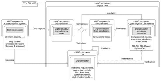
Figure 1.
Digital Twin and the V&V Loop.
The leftmost I4.0 Component, as shown in Figure 1, corresponds to the reference asset, and in our case, is the geographic area of Catalonia and its population. Using statistical tools, the data collected over time (the digital shadow) is the basis for building data-based models. In our case, we have used datasets from different countries to compare the results.
A daily process helps in the calibration of the simulation model using the data taken from the datasets. Hence, we can obtain an evolutive simulator that produces traces over time, which defines a virtual digital shadow. Therefore, the continuous comparison between the real asset’s digital shadow with the virtual simulator-generated digital shadow determines how the model must be calibrated or modified through the so called verification and validation loop (V&V Loop).
Because it is needed to perform a validation of the model continuously, the use of a standard formal language (SDL) that has a flowchart-like graphical representation, that is unambiguous (consistent) and complete, and has features that connect it to the IoT paradigm [25], simplifies this process. Essentially. SDL becomes the common language used to understand the model assumptions. We have ultimately developed a dashboard based on the Digital Twin Administration Shell, which is available at http://pand.sdlps.com (accessed on 14 July 2021).
2. Materials and Methods
As we mention, we develop three models to establish a validation through a model comparison approach. The first model is a classical SEIRD model and allows a fast conceptualization of the main model characteristics and features; this model is mainly used to test the preliminary assumptions and draw the model’s main boundaries. The second model, coded with Python, allows executing an optimization algorithm to find the points on the curve where the trend changes and calculate the transmission rate, a key parameter in our models. This model will accurately represent the trend of the pandemic situation in Catalonia, but that does not consider the real cases nor the confinement options, details we add on the SDL model. SDL and Python models must have similar behavior when comparing the variable Infective Detected (in the SDL model) and Infective (in the Python model). Both variables will also compare with the new cases time series obtained from the local authorities database [26]. In the following sections, we detail these three models and the interaction that exists between them.
2.1. System Dynamics Model
A classical SEIRD model is the basis of the system dynamics (SD) model, as depicted in Figure 2. We use this model to obtain a boundary that expresses the trend. These boundaries will be helpful to perform a validation based on the model comparisons approach [27] since the shapes and the trends of the other models will be similar to those obtained on this model. If not, we must reanalyze the models to detect the errors.
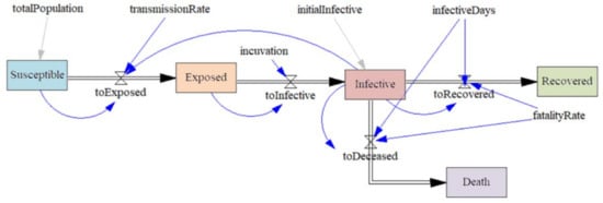
Figure 2.
SD models implemented in Vensim PLE.
Using this model, one can test the different assumptions faster, analyze the shape of the resulting curves and understand how the effects of the model modification, for example, the addition of new compartments, will affect the other models. We opt to keep this model as simple as possible, but it helps us define the boundaries of the forecast, the general trend, and the direction of the movement. Notice, however, that this model does not intend to make a forecast. It only serves as a basis for the discussions and becomes a tool for fast prototyping, in the initial stages of the model’s development. Essentially, it is used in the implementation stages to be able to detect errors in both coding or model definition through the model comparison approach.
The equations that drive the evolution of the model (Equations (1)–(5)) presented below represent the population variation of each compartment due to the flows between them, as shown in Figure 2, assuming that the total population remains constant (Equation (6)):
The (latency rate), (recovery rate) and µ (mortality rate) parameters will be considered constant, based on the measurements made by other studies, and N will be the total population, assuming that there is no pre-existing level of immunization to SARS-Cov2 and that therefore the whole population is initially susceptible ().
The mean incubation period () and the mean infectious period () come from the inverse of the above parameters. The fatality rate (µ) gives us the fraction of sick people who do not recover. The transmission rate (β) is the product of the contact rate per day and infectivity to make more detailed modeling. Finally, to calibrate β values, we will code a SEIRD model in Python.
2.2. Python Model
Python model runs an optimization model representing the different turning points that change the β we use on the SDL model. We use a simulated annealing algorithm called “dual annealing” included in the SciPy libraries to proceed with the multiparametric optimization by least-squares minimization [28]. In addition, we will also be able to estimate a value for the effective (Rt) and the basic reproduction number (R0) from the containment factor (), the transmission rate (β), and the recovery rate (γ) with the Equation (7). The basic reproduction number, R0, see [29], represents the average number of secondary cases that result from the introduction of a single infectious case in a susceptible population during the infectiousness period. The effective reproduction number, Rt, is the same concept but after applying the containment measures:
varies according to a confinement coefficient so that effective transmission rate can be calculated for each segment of the curve:
As input data, we have used the 7-day cumulative incidence and the number of turning points; using the Generalized Simulated Annealing algorithm also contained in the SciPy package [30] to optimize the values of the confinement coefficients () at the same time as the date on which they start to be applied. Thus, by establishing several turning points, we can reproduce different regimes of the epidemic curve depending on these non-pharmaceutical actions.
To fit the position of all the changing points and the transmission rate of each regime and ensure that the algorithm converges, we will proceed in a stepwise approach. So, we will consolidate the search boundaries of the previous fitted values to find the next ones and so on iteratively.
We selected this technique after trying several and finding that it worked well for us. The model allows randomly worsening the intermediate solutions to find a final solution closer to the global optimum. However, as the number of change points has increased, the difficulty of adjustment has also increased rapidly. Therefore, we end up approaching the problem in parts, so it would be interesting to improve the speed of the solution to look for other heuristics that could converge with a single execution and more efficiently. However, these alternatives are not needed at this point of the research since the time to obtain the solution is low, about one hour to do the whole process.
The main goal of the Python model is to estimate the changing points, as shown in Figure 3 that presents the different regimes on the curve. The aim is to define a model that behaves the same that the data we will obtain from the authorities (digital shadow). The assumption is that these points should correspond to the effect of the different government interventions such as confinements, reopening, distribution of masks, among others.
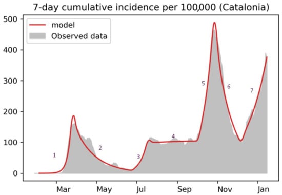
Figure 3.
Fitting the changing points to detect regime shifts in the cumulative incidence curve (7 regimes in this picture).
2.3. The SDL Model
Specification and Description Language (SDL) is a graphical object-oriented language with unambiguous formal semantics. The International Telecommunication Union standardized it. SDL uses four hierarchized building blocks: (i) SYSTEM, (ii) BLOCK, (iii) PROCESS, and (iv) PROCEDURES. Regarding the notation we use to describe the SDL diagrams, every time we refer to an SDL element, we write it in CAPS, while the name of the elements will be in Italic. The SYSTEM and BLOCK diagrams represent the model’s structure, using a hierarchical decomposition.
On the other hand, PROCESS and PROCEDURES define the model’s behavior. BLOCK and PROCESS are AGENTS that establish the communication sending SIGNALS through CHANNELS. SIGNALS act as a trigger, generating the execution of a set of actions in a PROCESS. All SIGNALS, sorted by time and priority in the input queue of every input channel, own a delay parameter that represents the time.
For those not used with SDL in the following Appendix A, we will detail the main elements of the language.
The SDL model is used to test the assumptions, and from them, effects of the NPIs. We define different models that incorporate these modifications. Table 1 shows the different models we develop in the frame of the project. All models are defined using SDL, but the modeling technique differs. 1.X models are the result of SD models, while 2.X models use cellular automaton (CA) structures, mainly to define the propagation in the different Health regions (a Health Region is an administrative division in Catalonia). 3.X models, not detailed here, are based on multi-agent simulation models (MAS) and are defined on SDL.

Table 1.
Models defined on the frame of the digital twin Catalonia’s pandemics modeling process.
Figure 4 shows the 2.5 SDL model BLayer BLOCK diagram. Squares (BLOCKS in SDL semantics) represent the different compartments. The semantics of the compartments is the same as in the SD or Python models, representing the Susceptible people and the Exposed people and so on. On the SDL model, we add some refinement with more compartments to better detail the population’s behavior, shown in grey. The main improvements of the SDL model are: (i) BLOCK BConfinement, representing the confined population excluded from becoming exposed. (ii) BLOCK BInfectiveDetected, representing the infected detected. We assume that over time the detection improves. (iii) BLOCK BContentionActions that controls the actions taken by the authorities to prevent SARS-CoV-2 spread. (iv) CA defines each cell as a model that details the spread of the SARS-CoV-2 over a Catalonia Health Region, Table 2.
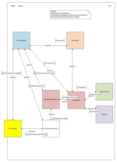
Figure 4.
SDL 2.5 model. Each color on the diagram represents a Compartment on the original SEIRD model (using the same colors). The exception is for the BContentionActions BLOCK that represents the different NPIs applied. Notice that BInfectiveDetected and BInfective refer to the single Infective compartment on the initial SEIRD model because on the SDL 2.5 version model, we can distinguish between real and detected cases. Notice that the 1(1) in the upper corner defines the number of pages that detail this diagram and the current page number.

Table 2.
Catalonia Health regions.
The use of the Health regions for validation allows us to see if the different curves for the different Health regions follow the data correctly. We keep the parameters that define the dynamics of the pandemic fixed and modify just the specificities of each health region, like the time of the first case or the population. A CA secondary layer details the number of persons included in each cell. Secondary layers represent static information needed for the model that remains unchanged during the model execution, like the initial total population for each health region.
As we mention, Model 2.5 is not the last model we develop; in SDL, model 2.9 represents the last refinement and contains other BLOCKS that allow us to describe the vaccination process accurately. To represent this vaccination process, we use the digital shadow of the system to introduce the vaccination rate on the model. Also, we can forecast the trend of this vaccination process to forecast the trend of the pandemic evolution. We can access the SDL model conceptualization at https://doi.org/10.6084/m9.figshare.13153100 (accessed on 14 July 2021).
3. Results
In this section, we present the process we follow to perform the continuous calibration of the models. We consider this process also a result since, through this discussion, we will be able to detect when and why a model is no longer valid, learning regarding the validity of the model assumptions we use.
3.1. Models Coding and Calibration
With the diagrams that compose the SDL model, one can implement it automatically with software that understands SDL, in our case using SDLPS (https://sdlps.com/ accessed on 14 July 2021). We define the same time discretization used in the SD model, using as the model time steep, following an activity scanning approach. Since the SDL model is the one that we will modify continuously, this automatic implementation will simplify the verification process (we can assume that the model implementation is correct).
To validate the model’s accuracy, we compare the daily new cases forecast with the dataset that contains the daily new cases in Catalonia. This dataset is available through the Open Data service in Catalonia (http://governobert.gencat.cat/en/dades_obertes/ accessed on 14 July 2021).
Since the model becomes a digital twin of the pandemic in Catalonia, it must include the NPIs applied to reduce the expansion of SARS-CoV-2. As we mention, these NPIs are part of the SDL model through events detailed on BContentionActions, defining a scenario parametrization.
3.2. Second Wave Calibration
To propose β values for a potential second outbreak, we use patterns of pandemic evolution in countries that have started earlier the school year, such as South Korea (August 25) or Israel (September 1), as shown in Figure 5.
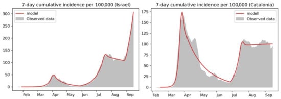
Figure 5.
SEIRD python-coded model results for Israel after the September 1 outbreak (top left) and for Catalonia before schools opening (September 14) (right). See the similarity in the patterns before the outbreak.
To estimate the β in those countries, we use our Python model. We have used the 7-day cumulative incidence to obtain the turning points representing the NPIs effects. The regimes are the first outbreak in spring, followed by a hard lockdown, a stabilization in summer, and a second outbreak after the academic year restart. Table 3 represents the parametrization for the SDL model version 2.5 that forecast the second wave. Several questions yet exist, like the percent of detection that will be estimated using the percent of asymptomatic [31].

Table 3.
Parameters for model 2.5 to be considered due to NPIs. % Det denotes real cases reporting level.
To estimate the percent of confinement, we use public data that allows calculating this percent. On March 15, the total closure of the country represents a maximum of 35% of confinement, but the return of the industrial sector implies 10% on April 13, 2020 [32]. For the second wave, October 10, the university population has been confined, these consist about 3% of the population, but we must increase this value on October 25 because leisure closes. Half of the public workers go online, representing about 7% more of the population, which is about 10% of the population that remain at home until November 23. To estimate the percent of detection, we use the prevalence study [31,33,34,35,36] for the 2.9 model, while for the previous models, we use an estimation based on [37,38].
Model 2.5 begins on January 29. On March 15, the government confined the entire population, except essential sector workers. On March 23, air space closes, on April 13, the industrial sector workers returned to work, and on April 20, the government gave all population basic masks. During May and June until July, the restrictions gradually decimated where we enter the “new normal.”
In Catalonia on September 14, we got . The time-series analysis shows that during the summer (that defines a sort of plateau), the value of β is peaking about 0.21, which can be considered a reference value for some kind of citizen’s behavior. The return to normality, with an increasing movement of citizens, can represent an inflection point. Different tests have been performed, concluding with a for 2.5 model, is this the value obtained from the analysis done in the Israel case, using the Catalonia cumulative incidence (85) and Israel (119), and considering that will be increased by the return to the normality and will become no smaller than the value of a total lockdown, see Table 4. We consider a 70% detection rate due to the increasing testing, being the 30% the asymptomatic rate we use [38].

Table 4.
β comparison. (*) In South Korea, the summer outbreak is so low that the model is not proper. (**) The forecast of a new outbreak with a β close to Israel proved to be accurate. (?) Information is not yet available, or the situation did not occur at the time of analysis of model 2.5.
Figure 6 shows the new infections forecast from the different scenarios that we ran on the SDL model. SDL attempts to forecast the maximum values (worst scenario).
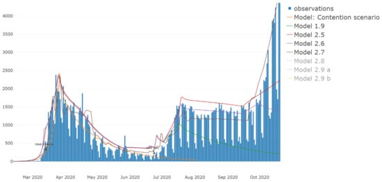
Figure 6.
Forecast for the new infections (y-axis), the red line for the 2.5 SDL model (being this an optimistic scenario). We consider other scenarios in case 2.5 model hypotheses fail, model 2.6, and model 2.7.
3.3. Third-Wave Calibration
For the calibration of the third wave, we use a historical data comparison to obtain more insights regarding the behavior of the pandemic in Catalonia. We define a new model named 2.8 that includes some new improvements over the previous models.
As in the previous models, we must define the β with the NPIs applied, selecting the same β that in the previous wave due to the coincidence on the scenario (schools reopening after the Christmas holidays). We use the β we apply on model 2.7 that represents model 2.5 with the adjusted β due to the observed cases.
Model 2.8 represents a new wave, but that does not show a uniform growth like on the second wave. That depends on how the people confine due to the Christmas holidays.
We detect one issue with the prevision during the validation process that does not invalidate the growth but avoids obtaining a better fit. We suppose that the growth does not continue to point A (see Figure 7) because we do not consider increasing the transmission due to increase contacts during the Christmas holidays. We suppose that remains at the same level observed in the summer, but clearly because now the people interact in a closed environment, this affects the transmission.
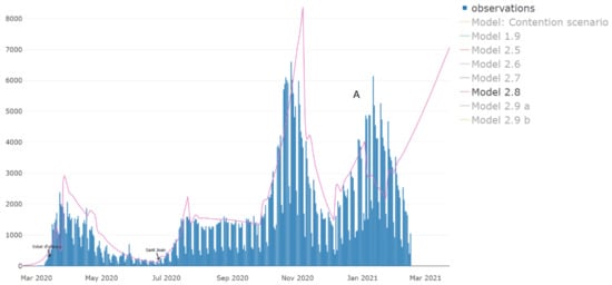
Figure 7.
Model 2.8 with the forecast for the second wave for the new cases (y-axis). Notice the divergence between the trend of the model and point A, the highest value of the data. We are presenting a scenario considering that the Christmas holidays have no acute effects on the β.
If we compare with the data, we see that the curve has an inflection point when the NPIs that include increasing the restrictions in the leisure sector (restaurants, theaters, among others) are applied, obtaining a β similar to the β we see on the descending trend of the second wave. Table 5 shows the parametrization for the 2.8 model.

Table 5.
Parameters used on the 2.8 simulation scenarios: (1) as a result of the validation process, the correct parameter for this β is 0.3, being added on the 2.9 model. (2) the organization of the online courses needs a week to be fully implemented.
New NPIs have been applied to the system, implying the modification of the β parameter, suggesting the need to revise the model hypotheses and the execution of the model following the continuous validation and verification loop.
4. Discussion
Applying a digital twin approach and focusing on a continuous validation of the model assumptions enables testing the possible causality effects for the NPIs applied to the population. The forecasts provided by the model seem accurate and allows us to understand the future evolution of the system. It will be a crucial aspect to size the resources needed at each stage of the pandemic evolution.
We calibrated the model to show always a pessimistic view of the situation. Notice that the forecast always tries to be over the observation’s maximum values. It will help decision-makers understand the worst scenario and prepare consistently for it.
We can access the dashboard to see the Key Performance Indicators (KPI’s) and model forecast, validated continuously against the actual data in a solution validation approach, becoming a digital twin of the pandemic. Figure 8 shows the dashboards for the model 1.9 prevision on September 16, previous to the publication of the 2.5 model.
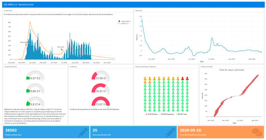
Figure 8.
KPIs for Barcelona and its health area CA cells Model 1.9.
When the model invalidates, a divergence between the digital shadows of the system (Catalonia SARS-CoV-2 new cases obtained from Socrata Open Data Source) and the master’s digital shadows (simulation traces) appears. Then, one must reevaluate the hypotheses and recalibrate the model, providing valuable information to understand the situation. It will happen continuously since new NPIs will be applied to control the spread of the virus. An interesting example of NPIs is when the government provides free masks to the population. This action seems to positively affect the population, which helps increase the confidence in the mask and change the population’s mindset.
By analyzing the different models, we can discuss the possibilities and the effects of the NPIs before their application on the system. As an example, model 2.5, with a , shows a scenario that is not optimistic but that presents a situation that implies an increase in the number of cases. Considering the model comparison approach and using the data we obtain from other countries, we see that the βs are highest than the proposed ones. At this point, the model suggests that if the growth happens, this will become faster, implying that a discussion based on models must include the needed analysis with different scenarios.
Another example is on model 2.8, where the situation presents the Christmas holidays, using for the analysis data that comes from our observations in Catalonia. We detect that the assumption that Christmas does not affect the β is not valid. The restoration reopening seems to impact the increase of the number of cases in the population. It has been detected and corrected on the 2.9 model using an accurate value for the β at this point. Notice that the current valid model, 2.9, correctly predicts the current trend of the pandemic in Catalonia, suggesting that the end of the cases will be possible at the end of the summer if the current conditions do not change (NPIs and no a variant with increased transmissibility appears). Figure 9 shows the forecast for the current trend of the pandemic situation in Catalonia using the current model.
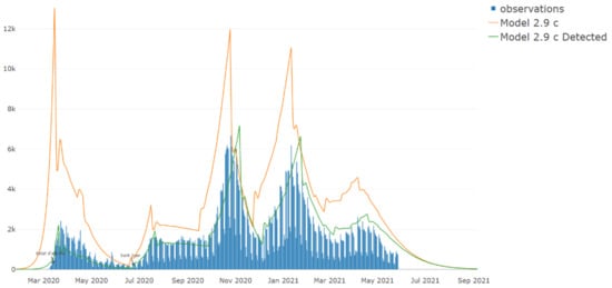
Figure 9.
Model 2.9 now forecasts for new cases (y-axis) the end of the pandemic situation in Catalonia if the NPIs remain similar to the current (at 05 June 2021) and no new variants appear.
This forecast again needs a continuous validation process but shows a positive effect of the vaccines for the disease contention. It suggests that the number of people who receive the vaccines will not have to reach 70% to achieve the desired herd immunity to control the spread; this time (05 June 2021), the number of people with complete vaccination is below 24%. We will confirm this scenario if the NPIs remain similar to the current or no new variants with the highest β appears. During the preparation of this document model, 2.9c was invalidated. The Delta variant spread and the reduction of some NPIs implied an increase in the number of cases in Catalonia. We therefore define a new scenario (2.9d) applying a β in our SDL model based on [39] and considering the reduction of the NPIs due to the reopening of the leisure [40] to be able to validate our forecast again. At this point, accurate monitoring of the epidemic using models will become an excellent tool to understand the implications and the effects of the NPIs if the situation worsens. Figure 10 shows the different models developed until now. Notice that every time an effective NPI is applied to the population, the model invalidates.
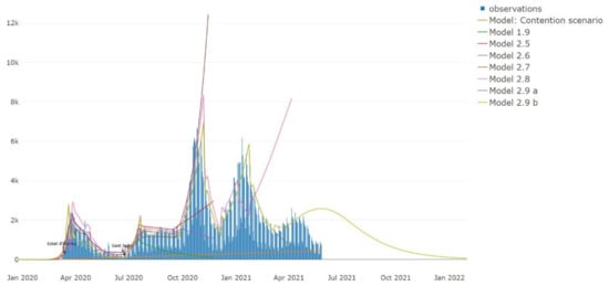
Figure 10.
The different models that we develop due to the continuous validation process, new cases (y-axis).
5. Conclusions
The current last model at the time of writing this paper, scenario 2.9c, needs accurate monitoring due to the inclusion of the vaccination effect in the model. An increase in the number of vaccines delivered every week to the population implies a substantial modification on the number of new cases detected later. Also, an eventual modification on the factors (NPIs, infectivity, among others) implies a necessary change of the model parameters to fit again with the system, following the shadows comparison of the digital twin approach.
The proposed methodology, defining a digital twin of the pandemic, must serve precisely to facilitate this monitoring, providing early warnings if the trend of the new cases differs from the trend of the forecasted model (shadows comparison). Because of the modification applied to the system, mainly the NPIs, to contain the virus spread, the representation of the model assumptions in a graphical language simplifies the immediate modification of the model. It makes easier the agreement between the different specialists involved in the project. This involvement of the specialists in the digital twin maintenance and continuous validation must serve to increase the model’s credibility, providing a way to achieve accreditation in a continuous verification and validation loop.
In the context of Industry 4.0, the model-based discussion becomes a central element to understand the causality of complex systems. The continuous validation of simulation models, which includes a clear representation of the causal relations, is part of the proposed methodology. We cannot make decisions without understanding the possible causality rules. Although we do not fully understand that the things happen as detailed in the model, the discussion based on these causal relations helps the decision-makers understand these rules, and more interestingly, when the assumptions and the hypotheses assumed on the model are not valid and must be reconsidered.
Author Contributions
Conceptualization, P.F.i.C., X.P.i.P. and J.G.i.S.; methodology, P.F.i.C.; software, V.G.i.C. and J.G.i.S.; validation, V.G.i.C., P.F.i.C. and J.G.i.S.; formal analysis, P.F.i.C. and V.G.i.C.; investigation, P.F.i.C., X.P.i.P. and V.G.i.C.; resources, P.F.i.C.; data curation, V.G.i.C., P.F.i.C. and J.G.i.S.; writing—original draft preparation, P.F.i.C., X.P.i.P. and V.G.i.C.; writing—review and editing, P.F.i.C., X.P.i.P. and V.G.i.C.; visualization, P.F.i.C. and V.G.i.C.; supervision, P.F.i.C.; project administration, P.F.i.C.; funding acquisition, P.F.i.C. All authors have read and agreed to the published version of the manuscript.
Funding
This research was partially funded by CCD, grant 2020-L015.
Institutional Review Board Statement
Not applicable.
Informed Consent Statement
Not applicable.
Data Availability Statement
The SDL 2.5 model conceptualization can be reviewed at https://doi.org/10.6084/m9.figshare.13153100 (accessed on 14 July 2021). and the model can be downloaded at https://figshare.com/articles/dataset/SDL-PAND_model_2_5/14910627 (accessed on 14 July 2021). The system’s dataset can be obtained at https://analisi.transparenciacatalunya.cat/ca/Salut/Registre-de-casos-de-COVID-19-realitzats-a-Catalun/xuwf-dxjd (accessed on 14 July 2021). Other SDL models can be accessed and downloaded at https://sdlps.com/Experiments (accessed on 14 July 2021), the results of the different scenarios can be accessed at http://pand.sdlps.com (accessed on 14 July 2021).
Acknowledgments
Thanks to the help of inLab FIB in the administration of the project.
Conflicts of Interest
The authors declare no conflict of interest.
Appendix A. SDL
Specification and Description Language (SDL) is an object-oriented, formal language. The International Telecommunication Union—Telecommunication Standardization Sector (ITU–T) defines it as a standard language. The document that defines the language structure is Recommendation Z.100. Originally the language was designed to specify event-driven, real-time, complex interactive applications that involve many concurrent activities. SDL bases the communication between the different model elements on the use of discrete signals [41,42].
The conceptualization of a simulation model needs to define the following components: (i) Structure: system, blocks, processes, and the hierarchy of processes, (ii) Communication: signals, including the parameters and channels that the signals need to travel from element to element, (iii) Behavior: defined through the processes. (iv) Data: based on Abstract Data Types (ADT), and (v) Inheritances: describe the relationships between and the specializations of the model elements. At least the first two components, the structure, and the behavior, must be described in a formal language to be able to do a correct conceptualization of a simulation model.
The language has four levels: (i) system, (ii) blocks, (iii) processes, and (iv) procedures.
A model always starts with the definition of what we want to represent. Using an approach based on a formal language, like SDL, we will start with a simple box that explains what the system to be modeled will be. This system, represented by the SYSTEM diagram, shows the uppermost level of the model’s structure. It clearly shows the elements that we consider in the analysis. All the other elements not present inside the SYSTEM diagram will become the ENVIRONMENT, and we express the communications between them using the CHANNELS. Following the SDL terminology, SYSTEM is an AGENT. Other AGENTS can appear in an SDL diagram, the BLOCKS, and the PROCESS. These other elements appear in lower levels of the model. The CHANNELS can be unidirectional or bidirectional and are using PORTS to connect with the BLOCKS or PROCESS. The PORTS guarantee the independence of the different AGENTS we will use in our models. It guarantees modularity, a crucial aspect of conceptual models since it allows us to reuse the different model elements. Also, modularity allows performing an incremental Validation and Verification process. It means that we do not need to Validate the whole model and focus on a subset of the model, a set of the model’s AGENTS. Because of modularity, an AGENT only knows what it sends and receives events using a specific PORT or CHANNEL.
To define a simulation model conceptualization, we need to detail the model structure and behavior. SYSTEM diagrams and BLOCK diagrams represent the model structure. It is a hierarchical decomposition of the different model elements; some good examples are available in [42]. The behavior will be described on the PROCESS diagrams and below, on the PROCEDURES, although these elements are not AGENTS and only represent some pieces of code. The pieces of information that travels on the CHANNELS, from AGENT to AGENT, are the SIGNALS. When a PROCESS receives a specific SIGNAL, it acts as a trigger, starting to execute a set of actions in no time. To represent the time, all the SIGNALS own a parameter, delay that represents when this SIGNAL can be processed. Every PROCESS has an input queue for every input CHANNEL, containing the received SIGNALS ordered by time and priority.
Being SDL a graphical language, a PROCESS uses different graphical elements to represent the model’s behavior. In the following lines, we describe some of the more essential elements synthetically to simplify understanding the SDL model definition.
Start.  This element defines the initial condition for a PROCESS diagram.
 This element defines the initial condition for a PROCESS diagram.
State.  The PROCESS must always start in a STATE, and this owns a name.
 The PROCESS must always start in a STATE, and this owns a name.
Input.  The PROCESS starts an execution when an INPUT receives the SIGNAL for this INPUT. All the STATES can own several different INPUTS to work with the different SIGNALS one can receive.
 The PROCESS starts an execution when an INPUT receives the SIGNAL for this INPUT. All the STATES can own several different INPUTS to work with the different SIGNALS one can receive.
Create.  This element allows the creation of an AGENT.
 This element allows the creation of an AGENT.
Task.  To interpret a piece of code, we can use the TASK element. In our approach, we can use C on this element.
 To interpret a piece of code, we can use the TASK element. In our approach, we can use C on this element.
Output.  To send a SIGNAL, we must use the OUTPUT element. We can also add parameters to the SIGNALS and describe the destination if ambiguity about the signal destination exists. We can direct the communication specifying destinations using a PROCESS identifier (PId), an identifier that must own all the PROCESS. Also, we can send using the sentence via path. We can use four PId expressions: (i) self, an agent’s own identity; (ii) parent, the agent that created the agent (Null for initial agents); (iii) offspring, the most recent agent created by the agent; (iv) sender, the agent that sent the last signal input (null before any signal received). Also, we can use {CUR_CELLS} and {ALL_CELL} to send the information to a specific cell of the CA.
 To send a SIGNAL, we must use the OUTPUT element. We can also add parameters to the SIGNALS and describe the destination if ambiguity about the signal destination exists. We can direct the communication specifying destinations using a PROCESS identifier (PId), an identifier that must own all the PROCESS. Also, we can send using the sentence via path. We can use four PId expressions: (i) self, an agent’s own identity; (ii) parent, the agent that created the agent (Null for initial agents); (iii) offspring, the most recent agent created by the agent; (iv) sender, the agent that sent the last signal input (null before any signal received). Also, we can use {CUR_CELLS} and {ALL_CELL} to send the information to a specific cell of the CA.
Decision.  To define a bifurcation, a decision point, we can use the DECISION.
 To define a bifurcation, a decision point, we can use the DECISION.
Finally, mention that on the last level of the SDL language (PROCEDURE diagrams), we can describe pieces of code, also graphically, making the language complete. We can use these pieces of code in the PROCESS with the PROCEDURE CALL  .
.
 .
.References
- Anderson, R. Discussion: The Kermack-McKendrick epidemic threshold theorem. Bull. Math. Biol. 1991, 53, 3–32. [Google Scholar] [CrossRef]
- Wynants, L.; van Calster, B.; Collins, G.S.; Riley, R.D.; Heinze, G.; Schuit, E.; Bonten, M.M.J.; Dahly, D.L.; Damen, J.A.; Debray, T.P.A.; et al. Prediction models for diagnosis and prognosis of covid-19: Systematic review and critical appraisal. BMJ 2020, 369, m1328. [Google Scholar] [CrossRef] [Green Version]
- Nava, A.; Papa, A.; Rossi, M.; Giuliano, D. Analytical and cellular automaton approach to a generalized SEIR model for infection spread in an open crowded space. Phys. Rev. Res. 2020, 2, 043379. [Google Scholar] [CrossRef]
- Chen, W.; Zhang, N.; Wei, J.; Yen, H.-L.; Li, Y. Short-range airborne route dominates exposure of respiratory infection during close contact. Build. Environ. 2020, 176, 106859. [Google Scholar] [CrossRef]
- Fonseca i Casas, P.; García i Carrasco, V.; Garcia i Subirana, J. SEIRD COVID-19 Formal Characterization and Model Comparison Validation. Appl. Sci. 2020, 10, 5162. [Google Scholar] [CrossRef]
- Ndaïrou, F.; Area, I.; Nieto, J.J.; Silva, C.J.; Torres, D.F. Fractional model of COVID-19 applied to Galicia, Spain and Portugal. Chaos Solitons Fractals 2021, 144, 110652. [Google Scholar] [CrossRef] [PubMed]
- Ogden, N.H.; Fazil, A.; Arino, J.; Berthiaume, P.; Fisman, D.N.; Greer, A.L.; Ludwig, A.; Ng, V.; Tuite, A.R.; Turgeon, P.; et al. Modelling scenarios of the epidemic of COVID-19 in Canada. Can. Commun. Dis. Rep. 2020, 46, 198–204. [Google Scholar] [CrossRef]
- Faniran, T.; Bakare, E.; Potucek, R.; Ayoola, E. Global and Sensitivity Analyses of Unconcerned COVID-19 Cases in Nigeria: A Mathematical Modeling Approach. WSEAS Trans. Math. 2021, 20, 218–234. [Google Scholar] [CrossRef]
- Arenas, A.; Cota, W.; Gómez-Gardeñes, J.; Gómez, S.; Granell, C.; Matamalas, J.T.; Soriano-Paños, D.; Steinegger, B. Modeling the Spatiotemporal Epidemic Spreading of COVID-19 and the Impact of Mobility and Social Distancing Interventions. Phys. Rev. X 2020, 10, 041055. [Google Scholar] [CrossRef]
- Lymperopoulos, I.N. SIR-Neurodynamical epidemic modeling of infection patterns in social networks. Expert Syst. Appl. 2021, 165, 113970. [Google Scholar] [CrossRef]
- Li, Y.; Campbell, H.; Kulkarni, D.; Harpur, A.; Nundy, M.; Wang, X.; Nair, H. The temporal association of introducing and lifting non-pharmaceutical interventions with the time-varying reproduction number (R) of SARS-CoV-2: A modelling study across 131 countries. Lancet Infect. Dis. 2021, 21, 193–202. [Google Scholar] [CrossRef]
- Flaxman, S.; Mishra, S.; Gandy, A.; Unwin, H.J.T.; Mellan, T.A.; Coupland, H.; Whittaker, C.; Zhu, H.; Berah, T.; Eaton, J.W.; et al. Estimating the effects of non-pharmaceutical interventions on COVID-19 in Europe. Nature 2020, 584, 257–261. [Google Scholar] [CrossRef] [PubMed]
- Ding, Y.; Huang, R.; Shao, N. Time Series Forecasting of US COVID-19 Transmission. Altern. Ther. Health Med. 2021, 27, 4–11. [Google Scholar] [PubMed]
- Maleki, M.; Mahmoudi, M.R.; Wraith, D.; Pho, K.-H. Time series modelling to forecast the confirmed and recovered cases of COVID-19. Travel Med. Infect. Dis. 2020, 37, 101742. [Google Scholar] [CrossRef]
- Vasiljeva, M.; Neskorodieva, I.; Ponkratov, V.; Kuznetsov, N.; Ivlev, V.; Ivleva, M.; Maramygin, M.; Zekiy, A. A Predictive Model for Assessing the Impact of the COVID-19 Pandemic on the Economies of Some Eastern European Countries. J. Open Innov. Technol. Mark. Complex. 2020, 6, 92. [Google Scholar] [CrossRef]
- Deb, P.; Furceri, D.; Ostry, J.; Tawk, N. The Effect of Containment Measures on the COVID-19 Pandemic. IMF Work. Pap. 2020, 20, 166. [Google Scholar] [CrossRef]
- Chen, S.; Prettner, K.; Kuhn, M.; Bloom, D.E. The economic burden of COVID-19 in the United States: Estimates and projections under an infection-based herd immunity approach. J. Econ. Ageing 2021, 20, 100328. [Google Scholar] [CrossRef]
- Sargent, R.G. Verification and Validation of Simulation Models. In Proceedings of the 2007 Winter Simulation Conference, Washington, WA, USA, 9–12 December 2007; pp. 124–137. [Google Scholar]
- Leiva, J.; Fonseca i Casas, P.; Ocaña, J. Modeling anesthesia and pavilion surgical units in a Chilean hospital with Specification and Description Language. Simulation 2013, 89, 1020–1035. [Google Scholar] [CrossRef]
- Vynnycky, E.; White, R. An Introduction to Infectious Disease Modelling; Oxford University Press: Oxford, UK, 2010; ISBN 978-0198565765. [Google Scholar]
- Fonseca i Casas, P.; Garcia i Subirana, J.; Garcia i Carrasco, V.; Silva de Barcellos, J.L.; Roma, J.; Pi, X. SDL Cellular Automaton COVID-19 conceptualization. In Proceedings of the 12th System Analysis and Modelling Conference on ZZZ; ACM: New York, NY, USA, 2020; pp. 144–153. [Google Scholar]
- Grieves, M.; Vickers, J. Digital Twin: Mitigating Unpredictable, Undesirable Emergent Behavior in Complex Systems. In Transdisciplinary Perspectives on Complex Systems; Springer: Berlin, Germany, 2017; pp. 85–113. [Google Scholar]
- Kritzinger, W.; Karner, M.; Traar, G.; Henjes, J.; Sihn, W. Digital Twin in manufacturing: A categorical literature review and classification. IFAC-PapersOnLine 2018, 51, 1016–1022. [Google Scholar] [CrossRef]
- Stark, R.; Kind, S.; Neumeyer, S. Innovations in digital modelling for next generation manufacturing system design. CIRP Ann. 2017, 66, 169–172. [Google Scholar] [CrossRef]
- Sherratt, E.; Ober, I.; Gaudin, E.; Fonseca i Casas, P.; Kristoffersen, F. SDL—The IoT Language. In Lecture Notes in Computer Science (Including Subseries Lecture Notes in Artificial Intelligence and Lecture Notes in Bioinformatics); Springer: Berlin/Heidelberg, Germany, 2015; Volume 9369, pp. 27–41. ISBN 9783319249117. [Google Scholar]
- Generalitat de Catalunya. Registre de Casos de COVID-19 Realitzats a Catalunya. Segregació per Sexe i Edat. Available online: https://analisi.transparenciacatalunya.cat/en/Salut/Registre-de-casos-de-COVID-19-realitzats-a-Catalun/qwj8-xpvk (accessed on 21 February 2021).
- Robinson, S.; Brooks, R.J. Independent Verification and Validation of an Industrial Simulation Model. Simulation 2009, 86, 405–416. [Google Scholar] [CrossRef]
- SciPy. scipy.optimize.dual_annealing. Available online: https://docs.scipy.org/doc/scipy/reference/generated/scipy.optimize.dual_annealing.html (accessed on 21 May 2021).
- Anastassopoulou, C.; Russo, L.; Tsakris, A.; Siettos, C. Data-based analysis, modelling and forecasting of the COVID-19 outbreak. PLoS ONE 2020, 15, e0230405. [Google Scholar] [CrossRef] [Green Version]
- Xiang, Y.; Gubian, S.; Suomela, B.; Hoeng, J. Generalized Simulated Annealing for Global Optimization: The GenSA Package an Application to Non-Convex Optimization in Finance and Physics. R J. 2013, 5, 13–28. [Google Scholar] [CrossRef] [Green Version]
- Pollán, M.; Pérez-Gómez, B.; Pastor-Barriuso, R.; Oteo, J.; Hernán, M.A.; Perez-Olmeda, M.; Sanmartín, J.L.; Fernández-García, A.; Cruz, I.; de Larrea, N.F.; et al. Prevalence of SARS-CoV-2 in Spain (ENE-COVID): A nationwide, population-based seroepidemiological study. Lancet 2020, 396, 535–544. [Google Scholar] [CrossRef]
- Taylor, L. Study Highlights Costa del Sol’s Malaga as One of the Best Quarantined Cities in Spain During Phase 0. Available online: https://www.euroweeklynews.com/2020/05/14/study-highlights-costa-del-sols-malaga-as-one-of-the-best-quarantined-cities-in-spain-during-phase-0/ (accessed on 12 July 2021).
- Ministerio de Sanidad estudio Ene-Covid19: Primera Ronda. Available online: https://www.mscbs.gob.es/ciudadanos/ene-covid/docs/ESTUDIO_ENE-COVID19_PRIMERA_RONDA_INFORME_PRELIMINAR.pdf (accessed on 14 July 2021).
- Ministerio de Sanidad Estudio Ene-Covid19: Segunda Ronda. Available online: https://www.mscbs.gob.es/ciudadanos/ene-covid/docs/ESTUDIO_ENE-COVID19_SEGUNDA_RONDA_INFORME_PRELIMINAR.pdf (accessed on 14 July 2021).
- Ministerio de Sanidad Estudio Ene-Covid: Informe Final. Available online: https://www.mscbs.gob.es/ciudadanos/ene-covid/docs/ESTUDIO_ENE-COVID19_INFORME_FINAL.pdf (accessed on 14 July 2021).
- Ministerio de Sanidad Estudio Ene-Covid: Cuarta Ronda. Available online: https://www.mscbs.gob.es/gabinetePrensa/notaPrensa/pdf/15.12151220163348113.pdf (accessed on 14 July 2021).
- Jung, C.-Y.; Park, H.; Kim, D.W.; Choi, Y.J.; Kim, S.W.; Chang, T.I. Clinical Characteristics of Asymptomatic Patients with COVID-19: A Nationwide Cohort Study in South Korea. Int. J. Infect. Dis. 2020, 99, 266–268. [Google Scholar] [CrossRef] [PubMed]
- Nishiura, H.; Kobayashi, T.; Miyama, T.; Suzuki, A.; Jung, S.-M.; Hayashi, K.; Kinoshita, R.; Yang, Y.; Yuan, B.; Akhmetzhanov, A.R.; et al. Estimation of the asymptomatic ratio of novel coronavirus infections (COVID-19). Int. J. Infect. Dis. 2020, 94, 154–155. [Google Scholar] [CrossRef] [PubMed]
- Reed, R. SDL-2000 for New Millennium Systems. Telektronikk 2000, 96, 20–35. [Google Scholar]
- Doldi, L. SDL Illustrated—Visually Design Executable Models, 1st ed.; TMSO Systems, Ed.; TMSO Systems: Old Main, PA, USA, 2001; ISBN 978-2951660007. [Google Scholar]
- Campbell, F.; Archer, B.; Laurenson-Schafer, H.; Jinnai, Y.; Konings, F.; Batra, N.; Pavlin, B.; Vandemaele, K.; van Kerkhove, M.D.; Jombart, T.; et al. Increased transmissibility and global spread of SARS-CoV-2 variants of concern as at June 2021. Eurosurveillance 2021, 26, 2100509. [Google Scholar] [CrossRef]
- Agencias Catalunya Levanta a Partir del Lunes la Prohibición de Celebrar Fiestas Mayores. Available online: https://www.lavanguardia.com/vida/20210604/7504929/catalunya-levanta-lunes-prohibicion-celebrar-fiestas-mayores-procicat-coronavirus-covid.html (accessed on 4 June 2021).
Publisher’s Note: MDPI stays neutral with regard to jurisdictional claims in published maps and institutional affiliations. |
© 2021 by the authors. Licensee MDPI, Basel, Switzerland. This article is an open access article distributed under the terms and conditions of the Creative Commons Attribution (CC BY) license (https://creativecommons.org/licenses/by/4.0/).