Non-Statistical Method for Validation the Time Characteristics of Digital Control Systems with a Cyclic Processing Algorithm

Abstract

The paper discusses the problem of performance and timing parameters with respect to the validation of digital instrumentation and control systems (I&C). Statistical methods often implicitly assume that the probability distribution law of the estimated parameters is close to normal. Thus, the confidence intervals for the parameter are determined on the grounds of this assumption. However, we encountered cases when the delay distribution law in I&C is not normal. In these cases, we used the non-statistical network calculus method for time parameters estimation. The network calculus method is well elaborated for lossless digital system models with seamless processing algorithm depending only on data volume. We consider the extension of the method to the case of I&C systems with considerable changes in the data flow and content-dependent processing disciplines. The model is restricted to systems with cyclic processing algorithms and fast network connections. Network calculus describes the data flow and system parameters in terms of flow envelopes and service curves that are generally unknown in advance. In this paper, we define equations that allow the calculation of these characteristics from experimental data. The correspondence of the Network Calculus and classical statistical estimation methods is discussed. Additionally, we give an example of model application to a real I&C system.

1. Introduction

Modern instrumental and control systems (I&C) for industrial facilities are implemented in most cases as a distributed digital environment. A number of approaches for the validation of the system’s timing and performance characteristics have been developed, and they vary depending on the available input data and experts’ theoretical backgrounds. Common techniques combine methods of statistical analysis and discrete mathematics [1,2,3,4,5]. The statistical methods usually assume that the distribution law of the measured parameters is close to normal [1]. In most cases, this assumption is valid for signals having a physical nature, but, as we will show, it can be false for signals describing the digital I&C itself, for example, data communication and information processing delays.

The network calculus method is one of the alternatives for evaluating computer network performance characteristics [6]. It is the non-statistical method of analyzing deterministic queuing systems based on mini-plus algebra and is attractive since it does not use assumptions about the probability distribution law of the values. The distinctive feature of the network calculus method is the use of specific functions to calculate delay and buffering parameters (service curves and envelopes of input and output data flow). Initially, network calculus was developed for the analysis of lossless digital streaming systems. The term lossless means that there are no data sources and sinks inside the system. Generally speaking, I&C systems do not belong to those systems since the following features characterize them:

• parallel processing of multiple tasks on same computing resource;
• significant change in the amount of information at the input and output of a component (for example, when a component compresses information);
• heterogeneity of data in a digital control system, in contrast to the information in streaming systems; it means that each element of data (bit) has its own value and can be processed according to a proper algorithm.

It is not to say that these features are not considered in the context of network calculus. The work [7] extends the method to systems with cyclic dependencies between input and output flows. Several works [8,9] give approaches for using network calculus in systems with significant differences between the input and output flow. Several papers [10,11] deal with various disciplines of joint processing of multiple tasks on a shared computing resource.

These approaches have common drawbacks. First, their application requires precise knowledge of the system’s internal features and, being tied to it, they are sensitive to any change in the system’s operating modes. Second, for complex systems, they lost the “transparency” of the results. Thus, a simple correlation with other characteristics (input data rate, burstiness, computational power of the component) becomes awkward.

In this paper, having analyzed these drawbacks, we develop a mathematical model of the digital I&C system. The model retains the generality and computational transparency with a possibility to take into account the uneven long-term relation between the input and output flows and heterogeneity of data. In the framework of the model, we investigated two subproblems that are of separate interest:

• comparing the network calculus computed delays with delays obtained by the statistical methods;
• calculation of the flow envelope and service curves from experimental data.

Both problems have not been adequately presented in the literature yet.

The model has been checked on simulated data and data obtained in a real I&C system [12].

2. The Structure of a Typical Industrial Automation Control System

The work considers a typical I&C system for an industrial facility (from now on, referred to as Control System—CS). The architecture of the CS has three levels (Figure 1):

• Equipment embedded controllers and low-level data gateways—level G (1);
• Data storage and data processing servers—level S (2);
• Human-machine interface components—level Z (3).

The $a\left(t\right)$ and $a^{*}\left(t\right)$ with numeric index are the input and output in a particular channel. A similar CS structure is used in various applications for real objects [12,13].

In accordance with the practical operating conditions of the CS at the facility, elements (G,S,Z) of the system implement a cyclic data processing algorithm.

Definition 1. 

A cyclic data processing algorithm is an algorithm with the following properties. At the start, the system element is in a state of waiting for the data to arrive. Sequentially incoming data packets are processed in a determined uniform way, and the system returns to its original state after the last packets in the sequence are processed.

For the cyclic algorithm, the total processing time of the data packet $D_C$ can be represented as the sum of two values:

$$D_C=T_E+T_S,$$

where $T_E$ is network delay $\mathrm{and} T_S$ is data processing time within system elements.

3. Application of Network Calculus to Evaluate Control System Time Characteristics

Let us consider the aspects of applying the network calculus method for computing time characteristics of a CS.

The network calculus [6] method was invented by Cruz [14,15] and is based on min-plus algebra (see [16]). The basic terms and notations of the method can be found in [6] or [17]. In this section, we present only the most important definitions.

Definition 2. 

A function$\beta$is the (minimum) service curve of a network element (or system) with the input flow$A$if$\beta$is a causal flow function and the element (system) output flow$A^{*}$satisfies:

$$A^{*}\ge A\otimes \beta ,$$

(1)

where$\otimes$is mini plus convolution operator.

Definition 3. 

A function$\gamma$is the (maximum) service curve of a network element (or system) with the input flow$\mathrm{A}$if$\mathsf{\gamma }$is a causal flow function and the element (system) output flow${\mathrm{A}}^{*}$satisfies:

$${\mathrm{A}}^{*}\le \mathrm{A}\otimes \mathsf{\gamma }.$$

(2)

Definition 4. 

A function$a$is the envelope of flow$\mathrm{A}$if$\mathrm{A}\le \mathrm{A}\otimes a$or, that is the same

$$a\ge \mathrm{A}\oslash \mathrm{A} ,$$

(3)

where$\oslash$is mini plus deconvolution operator.

The input and output flows are determined by the total amount of data registered at the input and output over a certain period. Therefore, the time of data passage through the system will accordingly be defined as the horizontal deviation $d\left(t\right)$ between these functions.

Definition 5. 

(The maximal delay in the system): For linear systems with input flow$\mathrm{A}$, the output flow${\mathrm{A}}^{*}$,$\mathrm{A}\left(\mathrm{t}\right)\ge { \mathrm{A}}^{*}\left(\mathrm{t}\right)$, the maximal delay${\mathrm{D}}_{\max }$expressed as the maximal horizontal distance between input and output flow curves is:

$${\mathrm{D}}_{\max }=\mathrm{h}\left(\mathrm{A},{\mathrm{A}}^{*}\right)=\underset{\mathrm{t}\ge 0}{\sup }\left\{\inf \left\{\mathrm{d}\ge 0:\mathrm{A}\left(\mathrm{t}\right)\le {\mathrm{A}}^{*}\left(\mathrm{t}+\mathrm{d}\right)\right\}\right\},$$

(4)

One of the crucial points of network calculus is that the maximum value of delay ${\mathrm{D}}_{\max }$ can be obtained using bounds rather than real cumulative functions, see the proof in [6]:

$${\mathrm{D}}_{\max }=\mathrm{h}\left(\mathrm{a},\mathsf{\beta }\right),$$

(5)

where $\mathrm{h}$ is the maximal horizontal distance between two curves.

4. Network Calculus Main Curves Estimation Approaches

Let us consider the problem of determining the flow envelope, the minimum and maximum service curves of the system, and their linear approximations based on the flow data measured during the experiment.

4.1. Calculation of the Flow Envelope Based on Experimental Data

Equation (3) defines a direct method for calculating the envelope of the cumulative flow $A$. It is convenient to deal with a piecewise linear approximation of the envelope, which is reduced to the affine function $y=kx+b$ in some cases. The piecewise linear approximation allows using effective computational algorithms of data processing [18,19]. The affine function approximation allows to quickly perform system analysis and make numerical estimations of the system behavior [10]. The flow envelope approximation in the form of an affine function in the Network Calculus method was considered in [20]. The work [21] considers methods for calculating a one-component linear flow envelope based on support vector machine algorithms.

4.2. Maximum and Minimum Service Curves Calculation Approaches Based on the Experimental Data

Determining the parameters of the service curve is not as easy as for envelope. Theoretically, we could get service curves as a strict bound using specially designed test flow and taking into account the convolution property when zero element for ∧ is absorbing for mini plus convolution operator ⊗ [6]. However, the experiment is unrealistic because it would require a flow described by $\delta \left(t\right)$, that would overload any real system.

The second approach is using a relation between mini deconvolution and convolution operators [6]:

$$C\ge B\oslash A\iff B\le A\otimes C,$$

(6)

Using (6) and the definition of min plus deconvolution [6], we obtain a lower bound for the maximum service curve:

$${\gamma }^{\prime }=A^{*}\oslash A,$$

(7)

where $A$ and $A^{*}$ are input and output flow, respectively.

Meanwhile, the estimation of only the maximum service curve is often not sufficient for system analysis. For example, the calculation of maximal system delay and buffer size requires the minimum service curve (1). We are not aware of any satisfactory methods of experimental minimum service curve calculation.

Below, we will introduce an approach to the calculation of the minimum service curve. It is similar to the approach of maximum service curve calculation, but uses a “weak” property that we are going to prove.

Proposition 1. 

Let$A,B,C\in \mathcal{F}$and if$C\le B\overline{\oslash }A$, then

$$B\ge A\otimes C,$$

(8)

Proof. 

Let $C\left(s\right)\le \left(B\overline{\oslash }A\right)\left(s\right)$ for $s\in ℝ$. Let us write explicitly for some $s,v\ge 0$:

$$B\left(s+v\right)-A\left(v\right)\ge \underset{u\ge 0}{\inf }\left(B\left(s+u\right)-A\left(u\right)\right)\ge C\left(s\right),$$

or

$$B\left(s+v\right)\ge C\left(s\right)+A\left(v\right),$$

(9)

$$t=s+v$$

Rewrite (9) as

$$B\left(t\right)\ge A\left(t-s\right)+C\left(s\right),$$

(10)

The inequality (10) is valid for any s, $t\ge s\ge 0$; it is also valid for some $s$ where the expression gains the low boundary, that is

$B\ge A\otimes C$, $\forall t\ge 0$. □

The proved proposition allows us to estimate the minimum service curve. Let $A$ be cumulative input flow, $A^{*}$ be cumulative output flow. Then, by virtue of the proved proposition for the curve:

$${\beta }^{\prime }=A^{*}\overline{\oslash }A,$$

(11)

The inequality $A^{*}\ge A\otimes {\beta }^{\prime }$ is satisfied; it means, in turn, that ${\beta }^{\prime }$ is the estimated minimum service curve ${\beta }^{\prime }\le \beta$.

Since property (8) is only a necessary condition, the estimation of the minimum service curve obtained by Equation (11) can lie both above and below the real minimum system service curve. Comparing Equations (6) and (8), we also note that ${\beta }^{\prime }\le {\gamma }^{\prime }$, i.e., the minimum service curve is bounded from above with the maximum service curve. Note, partially the result of the Equation (16) might be negative. Then we consider for a physically realizable system only the positive part: $\max \left(0,{\beta }^{\prime }\right)$.

In a particular case, when a system does not have a maximum service curve (i.e., when there is a mode of “instant” processing of the input data), it is possible to obtain an exact value for the minimum service curve by using the envelopes instead of the input and output cumulative flow. To do this, let us assume that $\alpha , {\alpha }^{*}$ are envelopes of the input and output flows, respectively. It is known that ${\alpha }^{*}= \left(\alpha \otimes \gamma \right)\oslash \beta$ (see [6] p. 34). Then the equation $\gamma \left(t\right)=\delta \left(t\right)$ can be rewritten as:

$${\alpha }^{*}=\alpha \oslash \beta ,$$

(12)

and by the property of the operator $\oslash$ (see [6] p. 123) and the minimum service curve $\beta$:

$$\alpha =\beta \otimes {\alpha }^{*},$$

Using the commutativity of the operator $\otimes$ and applying the same property in the reverse direction, we obtain the estimation of the minimum service curve:

$${\beta }^{\prime }={\alpha }^{*}\oslash \alpha ,$$

(13)

If the service curves can be described by affine functions, then there are fast convolution and deconvolution algorithms for them, which are necessary for calculating system parameters [11]. As shown in [22], the service curves can be approximated by the affine functions similar to the flow envelope and with the same algorithms based on the support vector machines algorithm.

5. I&C System Model and CS Time Characteristics Validation

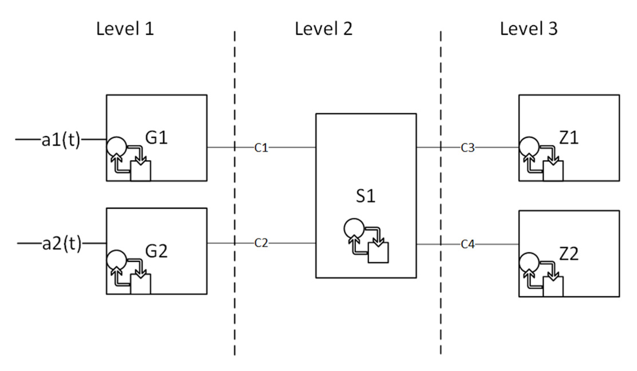
Let us consider a problem of modeling a typical CS presented in Figure 1 using the network calculus framework. Additionally, let us suppose the CS has excessive computing resources. This allows us to decompose the system and consider each logical channel of the system separately. If this condition is not met, it is necessary to take into account the discipline of resource sharing (see, for example, one of the of the task scheduler models [11]). 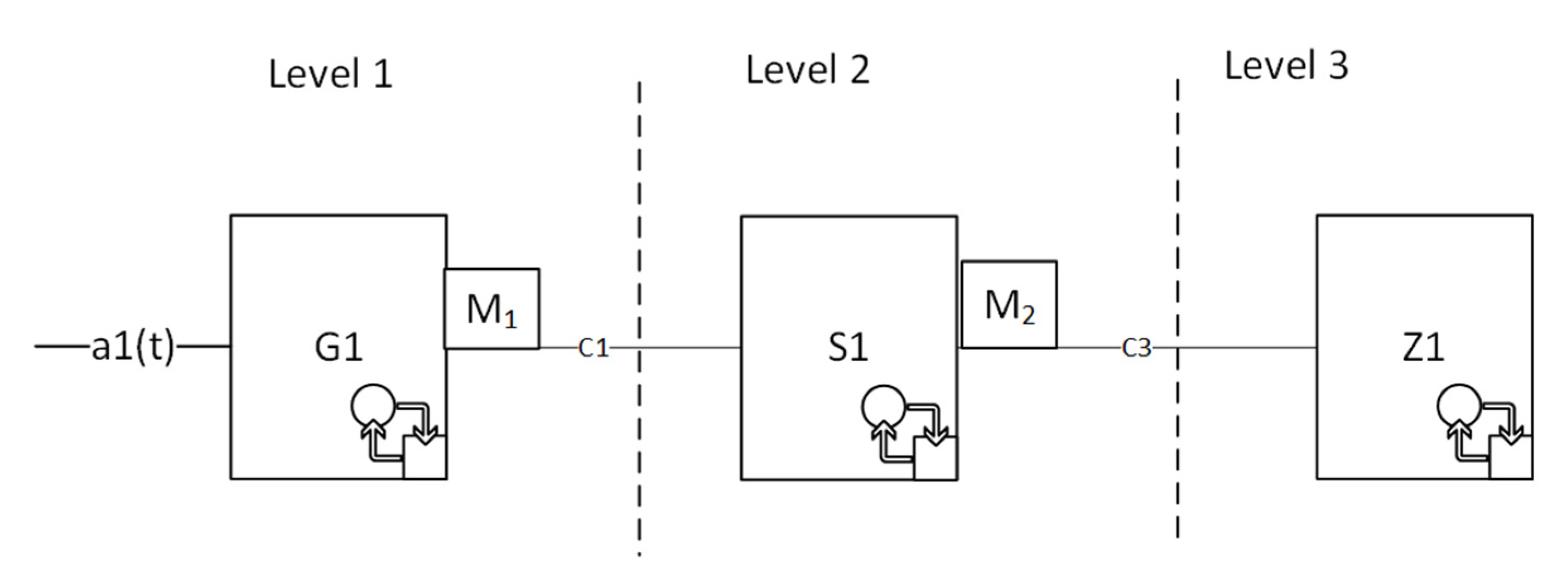Figure 2 shows a separate channel of a CS. Each component in the channel has its own maximum and minimum service curves.

All main conclusions and equations in the section will be given for the minimum service curve. As follows from the definitions of the maximum and minimum (1, 2) service curves, the conclusions and equations for the maximum service curve will be similar and can be written by simply renaming the variables and replacing the inequality signs in the relations.

To designate a specific component, we will add a lower alphanumeric index to $\beta$ following the notation in Figure 2. Cumulative input and output flows at each component will be denoted as $A,A^{*}$.

Then, in accordance with the definition of minimum service curve (2), for every system element, we can write an expression in the following form:

$$A^{*}\ge A\otimes \beta$$

However, in practice, all CS elements’ characteristics, except the communication conduits, are not linear; the scale of the flow changes between the input and output. For example, a single alarm signal at the component input can cause an avalanche of related signals, which will lead to an increase in information at the output of the component. To describe the change in the flow scale, the scaling function $M$ and its inverse function $M^{-1}$ are introduced into the model (Figure 2). The scaling function provides the transformation $M:A^{*}\to A$ and $M^{-1}:A\to A^{*}$ [8]. So, the service curve of the ${\beta }_{Si}$ system for the $i$-th channel with regard to the scaling functions is expressed as:

$${\beta }_{Si}={\beta }_{Gk}\otimes M_1{}^{-1}({\beta }_{Cn1}\otimes {\beta }_{Sl}\otimes M_2{}^{-1}({\beta }_{Cn2}\otimes {\beta }_{Zm}))$$

(14)

where $i,k,l,m,\in \mathrm{N}$ are indexes of connected in sequence components in a data processing logical channel at each CS level; $n1,n1\in \mathrm{N}$ are the indexes of communication channels used in data transmission between the components in the channel $i1$; and $M_1, M_2$ are the scaling functions of the corresponding components. The service curves ${\beta }_{Cn1}, {\beta }_{Cn2}$ reflect the network data transmission delay $T_E$, and the rest refers to the data processing delay $T_S$ in the component.

Provided that service curves calculation and scaling functions for each of the components is possible, Equation (14) allows to obtain the bounds for data processing delay in the entire system, depending on the characteristics of the input flows $ai\left(t\right)$, $i\in \mathrm{N}$. However, in practice, calculating the scaling functions $M$ of a real system is a complicated and not always solvable problem.

To avoid difficulties with the definition of scaling functions, we will redefine the input and output flows and move from real flow to virtual one for systems with a cyclical data processing algorithm.

Let us suppose all data received by the system at the beginning of each cycle will be processed and transmitted to the output by the end of the cycle, and consider the following function:

$$\left\{\begin{array}{c}q\left(j\right)={\tau }_j,j\in \mathbb{N}\\ q\left(0\right)=0,\end{array}\right.$$

where $j$ is the number of the cycle, ${\tau }_j$ the cycle, and $j$ duration. Next, let introduce on an interval $\left[\left.0,+\infty \right)\right.$ a step function $Q\left(x\right)$:

$$Q\left(x\right)={\displaystyle \sum }_{l=0}^{j}q\left(l\right),j\le x<j+1$$

The step function $Q\left(x\right)$ is by definition a flow function.

The output flow $Q^{*}$ for a component can be obtained from the input flow by shifting it to one cycle:

$$Q^{*}\left(x\right)=\left\{\begin{array}{c}Q\left(x-1\right),x\in \left[1,+\infty \right)\\ 0,x\in \left[0,1\right)\end{array}\right.$$

(15)

Note: the definition of the maximal delay for virtual flows must be redefined as:

$${\mathrm{D}}_{\max }=\mathrm{v}\left(\mathrm{Q},{\mathrm{Q}}^{*}\right)=\underset{\mathrm{t}\ge 0}{\sup }\left\{\mathrm{Q}\left(\mathrm{t}\right)-{\mathrm{Q}}^{*}\left(\mathrm{t}+\mathrm{d}\right)\right\}.$$

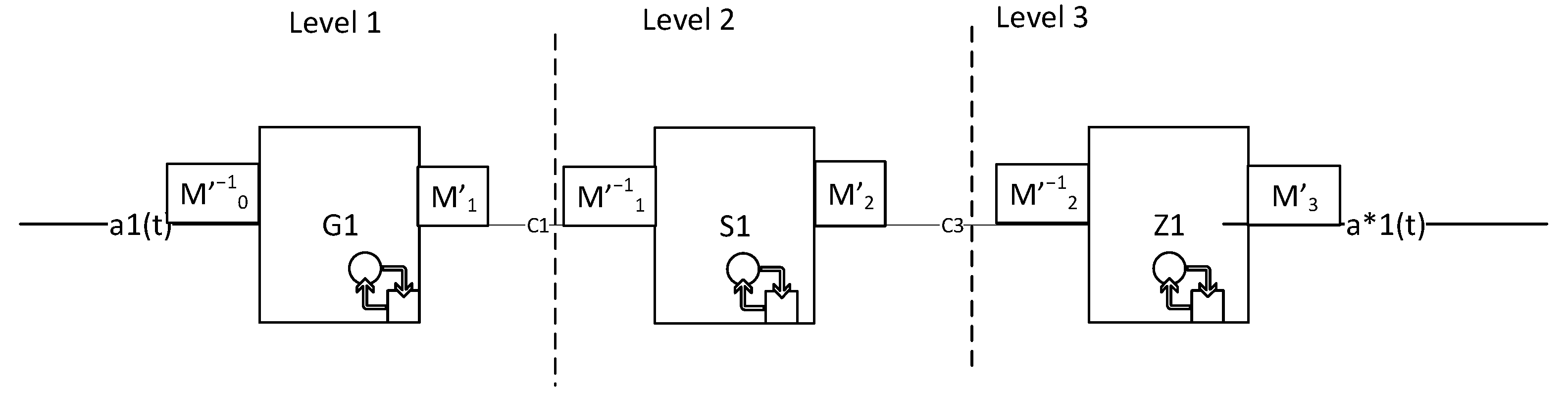
The structural diagram (Figure 2), redefined for virtual flows in components of the G, S, Z type, is shown in Figure 3.

For a channel with “virtual” flows for components G, S, Z, we redefine the meaning of service curves $\beta$ and $\gamma$ as:

$$Q^{*}\ge Q\otimes \beta$$

$$Q^{*}\le Q\otimes \gamma$$

and introduce mapping operators: $M_0{}^{\prime },M_1{}^{\prime }, M_2{}^{\prime }$ providing the transformation $M^{\prime }:Q^{*}\to A$, and the inverse mapping operators providing the transformation ${M^{-1}}^{\prime }:A^{*}\to \mathrm{Q}$. Then the service curve for the system shown in Figure 3 will look like this:

$${\beta }_{Si}={\beta }_{Gk}\otimes M_1{}^{\prime }\otimes {\beta }_{Cn1}\otimes M_1{}^{-1^{\prime }}\otimes {\beta }_{Sl}\otimes M_2{}^{\prime }{\beta }_{Cn2}\otimes M_2{}^{-1^{\prime }}\otimes {\beta }_{Zm},$$

(16)

In turn, Equation (16) can be reduced (see [8] Section 5.1) to a more convenient form by transferring the scaling functions $M^{\prime }$ from the input to the output of the component and omitting the pair $M^{\prime },{M^{-1}}^{\prime }$ by component output:

$${\beta }_{Si}={\beta }_{Gk}\otimes M_1{}^{-1^{\prime }}({\beta }_{Cn1})\otimes {\beta }_{Sl}\otimes M_2{}^{-1^{\prime }}({\beta }_{Cn2})\otimes {\beta }_{Zm},$$

(17)

The partial transition from $A$ to $Q$ in Equations (16) and (17) does not generally simplify the work with the scaling functions. However, if:

$${\beta }_{\mathrm{C}i}\gg {\beta }_{\left\{G,S,Z\right\}i}$$

(18)

one can replace ${\beta }_{\mathrm{C}i}$ by a function that is neutral with respect to the mini-convolution operator $\delta \left(t\right)$:

$$\delta \left(t\right)=\left\{\begin{array}{c}0, t=0\\ +\infty , t>0\end{array}\right.,$$

with the following property: $f=\delta \otimes f$ (see, for example, [6]).

For a monotonic scaling function:

$$M^{-1^{\prime }}\left(\delta \left(t\right)\right)\to \delta \left(n\right), n\in \mathrm{N}$$

it becomes possible to omit ${\beta }_{\mathrm{C}i}$ from Equation (17) and, accordingly, to get rid of the scaling functions. Physically, the Assumption (18) means that the processing cycle time in the network stack and the time of information transmission over the system network are negligible compared to the time of information processing on a computing resource. This assumption is mainly fulfilled in modern CS, where the transmitted information has a relatively small volume compared to the bandwidth of communication channels.

In this case, the overall system service curve in Equation (17) for the $i$-th chain for the “secondary” virtual flow is simplified:

$${\beta }_{Si}={\beta }_{Gk}\otimes {\beta }_{Sl}\otimes {\beta }_{Zm},$$

(19)

where $k,l,m\in \mathrm{N}$—are the indexes of sequentially connected components.

6. Network Calculus Method Application Verification for System’s Time Characteristics Estimation

6.1. Reference Data and Verification Procedure

The delay is calculated using an input flow envelope and service curve, which are not measured directly but are the result of calculations. It is clear that the methods used to compute them will also affect the trustworthiness of the final result. Therefore, let us focus on the practical aspects of the delay computation and compare the results of network calculus and statistical analysis.

The network calculus method was verified using test data with known statistical parameters. The test program simulates the CS component with a cyclic operation algorithm. The network delay $T_E$ and cycle time $T_S$ were random variables distributed according to a certain law. For data analysis, we use the free network calculus library [10].

6.2. Comparing the Network Calculus and Statistical Results

For each sample, we compute:

• delay ($D$) calculated by the network calculus (5) using experimental maximum and minimum service curves;
• maximum measured delay in the sample ($D_x$);
• ratio of $D/D_x$;
• dependence of the maximum calculated delay on the sample size ($L)$ and distribution.

The data in the samples have different distributions, including distributions that were close to normal and those with heavy tails. In the experiments we assume that the data was completely processed: $\exists t_e\ge 0, A\left(t_e\right)=A^{*}\left(t_e\right)$. All data presented have been rounded to ~1%. When using the distribution law with possible negative values, the negative data were discarded.

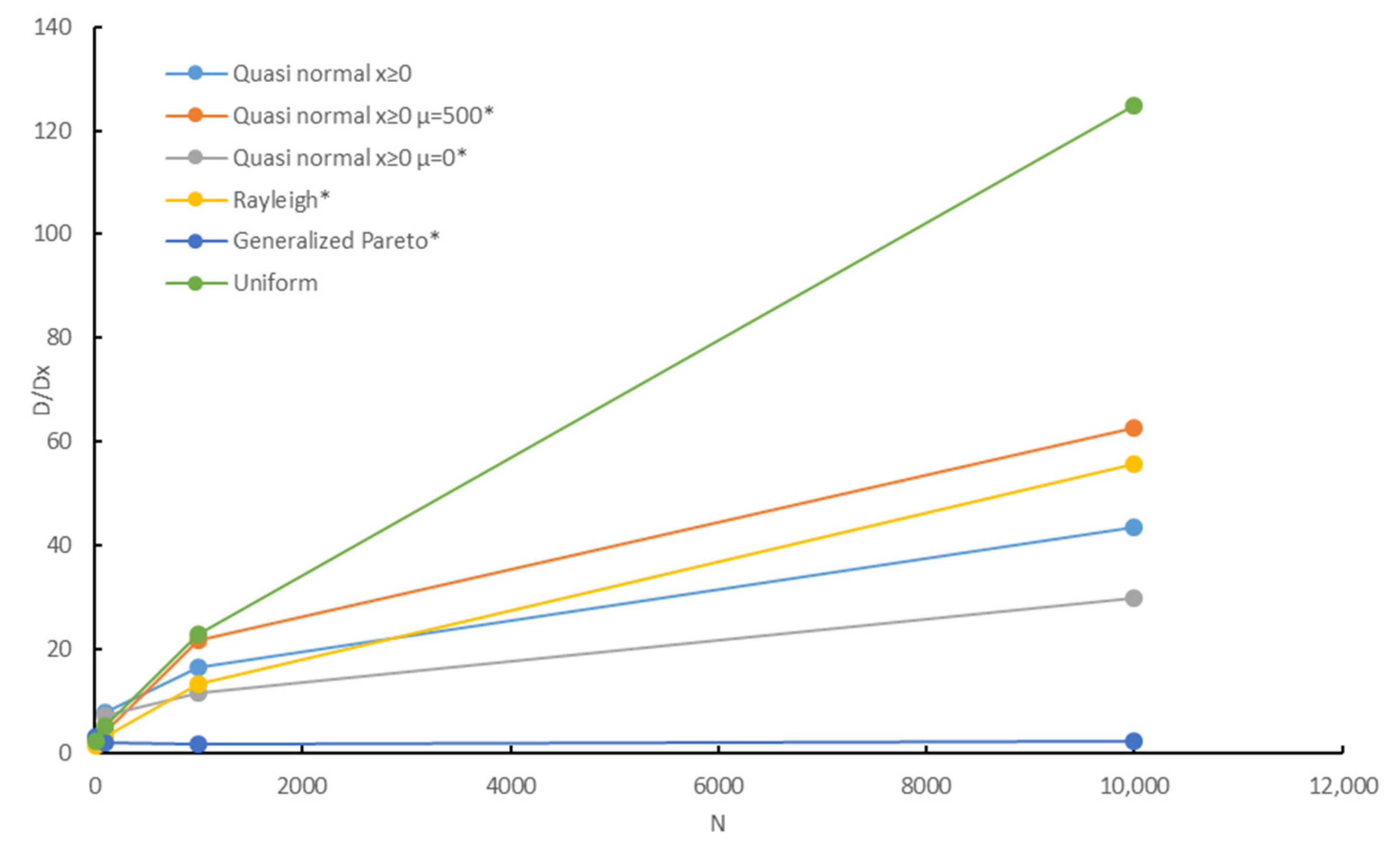
Figure 4 shows the dependence of the ratio $D/D_x$ on the sample size for different probability distribution functions, where $D$ is the maximum delay in the network calculus method with the service curve calculated by Equation (13).

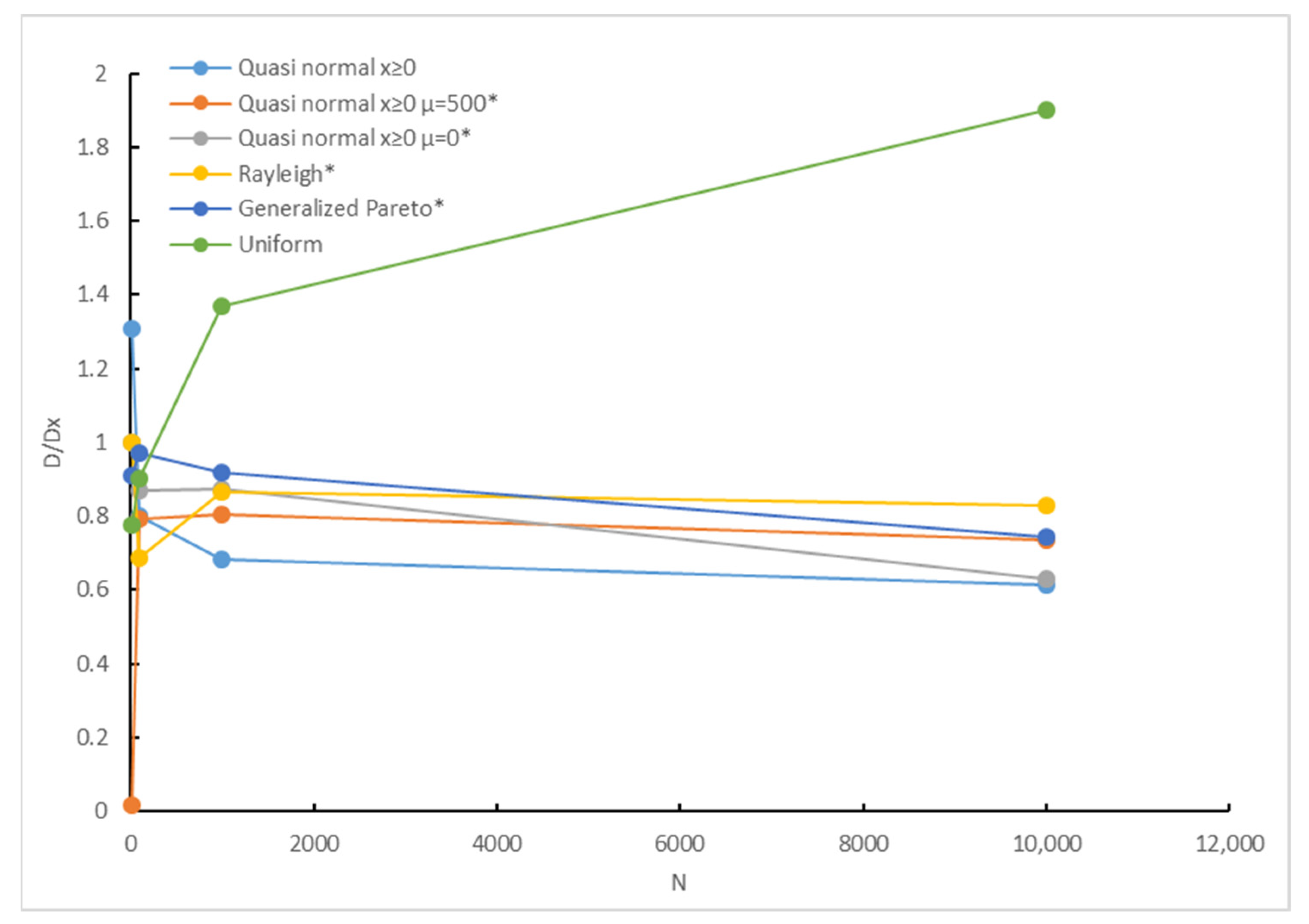
Figure 5 shows the dependence of the ratio $D/D_x$, where $D$ is the calculated maximum delay in the network calculus method with the service curve calculated with the use of Equation (7) for different probability distribution functions and sample sizes.

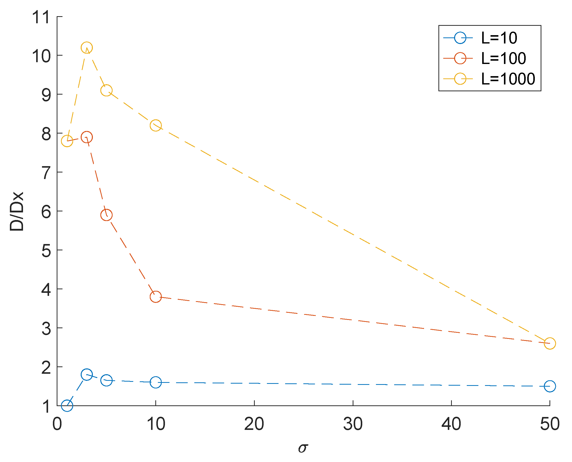
The dependence of $\frac{D}{D_x}$ on the sample size and outlier amplitude using the minimum service curve is shown in Figure 6.

The experiments allow us to make the following observations and conclusions about the relation of the statistical and network calculus results.

The maximum delay estimation with the use of a minimum service curve (13) is more accurate for short samples (Figure 6) and heavy-tailed distributions (Figure 4). The $\frac{D}{D_x}$ ratio increases with increasing sample size, although the rate of delay changes decreases with the increasing sample. The $\frac{D}{D_x}$ ratio can be as high as ${10}^2$.

Meanwhile, the simulation shows that the maximum delay calculated with the use of service curve (7) characterizes the delay in the normal operating mode (Figure 5). The delay is close to the maximum delay in the sample and depends weakly on the sample size for sufficiently large samples.

The maximum delay estimation with the use of service curve (7) is close to the experimental maximum delay $D_x$ but $D$ is commonly somewhat less than $D_x$. The resulting estimate better correlates with the real maximum delay during an increase in the sample size and for distributions close to normal (Figure 5).

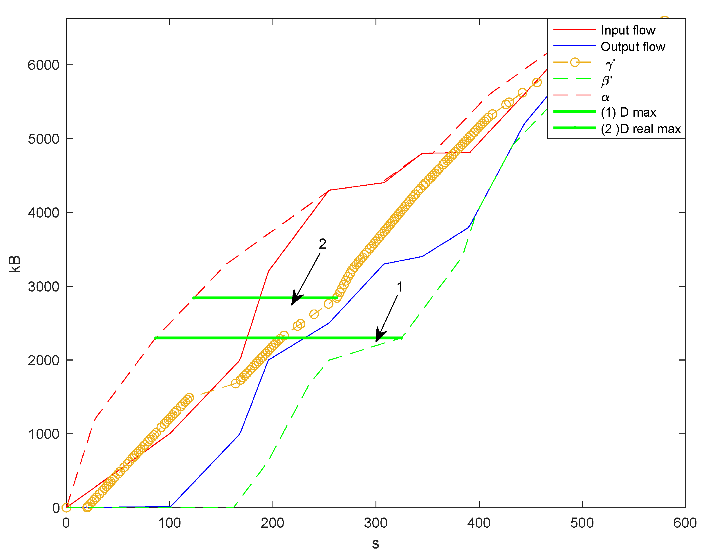
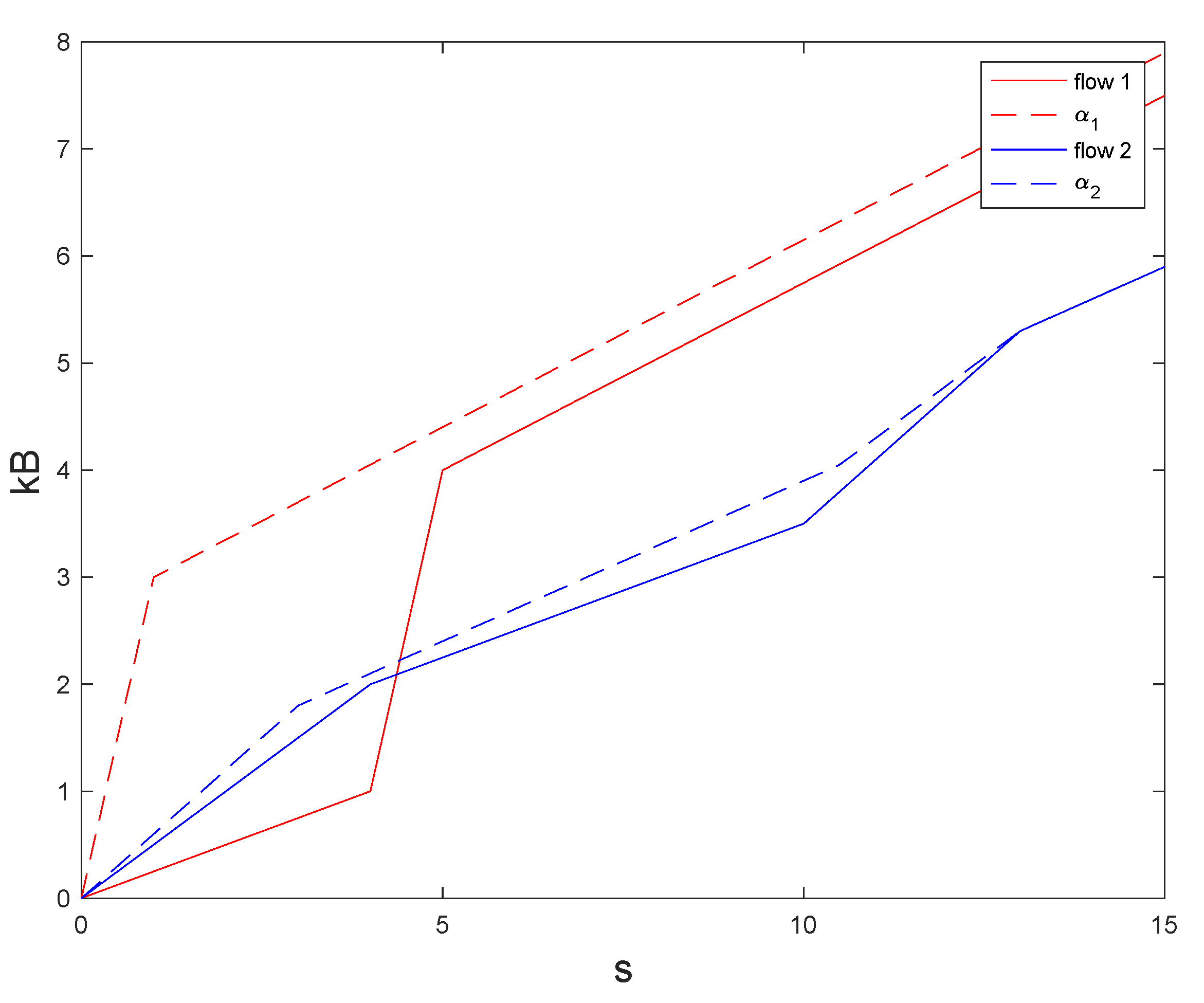
Figure 7 shows a typical shape of the network calculus curves obtained from the experimental network data. The sample data follow quasi-normal distribution with $\mu =500,\mathsf{\sigma }=100$. For clarity, the data of a short size are given. The lower horizontal line corresponds to the maximum delay calculated for the maximum service curve (7). This delay is close to the maximum sample delay. The upper horizontal line corresponds to the estimation of the maximum delay for the maximum service curve (11). The figure clearly shows that the input flow envelope limits all curves on the figure from above, and an estimation of the minimum service curve limits them from below.

6.3. Comparison of Network Calculus and Statistical Calculation Results

Our simulations have shown that the $\frac{D}{D_x}$ ratio values and the maximum delay depend on the probability distribution law of processing time and on the sample length and the number and amplitude of individual outliers in the data.

The dependence is complex due to the non-linear nature of the formulas describing the basic operations. According to them, the flow envelope and service curve will have sections composed of data close in value, sorted in descending order for the flow envelope and the maximum service curve and ascending for the minimum service curve (см. [6] p. 113).

Thus, with the sample length increase, the flow will contain a larger number of sections with a significant steepness. Therefore, both the flow envelope (8) and the service curves are calculated by Equations (7) and (11) will change.

The maximum service curve (7) estimation from the sample will have similar behavior with the flow envelope. The minimum service curve has an opposite tendency (Figure 7). Therefore, maximum delay estimation by Equation (7) is less dependent on changes in the input data and the length of the sample.

A heavy-tailed probability distribution law is characterized by the presence of a certain number of outliers, which are very different from the rest of the values. For distributions close to normal, the appearance of such outliers in the sample is less likely, but they are nonetheless characterized by the presence of a sufficient amount of data within the confidence interval. So, the overall curvature trend for the envelope and service curves will differ depending on data distribution. For samples with single large outliers, the curves will have large curvature at the beginning and a subsequent sharp decrease. For samples without large outliers, the curvature will decrease smoothly (Figure 8).

This lets us understand the relationships between the delay estimation obtained from the network calculus and classical methods of statistical estimation (see, for example, [23]).

It is known [24] that network calculus implicitly assumes the worst combination of conditions for information processing in the system. Graphically, it means that the beginning of the envelope curve consists of areas with the most significant changes in the input flow (i.e., a worst-case scenario that can be predicted from the observed data). For the delay based on the minimum service curve, the worst-case scenario is also the arrival of the largest packet of data when the server is busy and has low performance. When calculating the delay with the maximum service curve, the maximum data size corresponds to the maximum service performance (i.e., when the maximum amount of data accompanies the system’s maximum performance), which is typical for the system’s normal operation.

In both cases, the delay calculated using network calculus corresponds to the delay calculated for the two described scenarios for statistical methods of calculation. The probability that an actual delay will reach this value corresponds to the probability of this scenario being realized in the experiment.

For verification, we calculated the probability that the real delay will be less than the delay calculated by the network calculus method. For the delay calculated using the minimum service curve, in most cases, as expected, this probability is close to the unity.

7. Practical Example of Calculating the Delay for a Real I&C System

This section presents the results of evaluating the time characteristics of the actual control system described above (Figure 1). In order to substantiate the possibility of using the simplified Formula (18) for calculating the service curve of the entire system, the network delays of data transmission between the components were also measured. For the measured values, empirical probability distributions are calculated, and for the network delay, spectral characteristics are additionally analyzed.

Measurements were carried out for elements of level Z (from Figure 2). The amount of cyclic data being processed is relatively stable under normal operating conditions and has some average speed. However, with some special (actuation of protections and equipment interlocks) or transient processes (transition from mode to mode), the amount of data and the algorithm (that is, speed) of processing can change significantly.

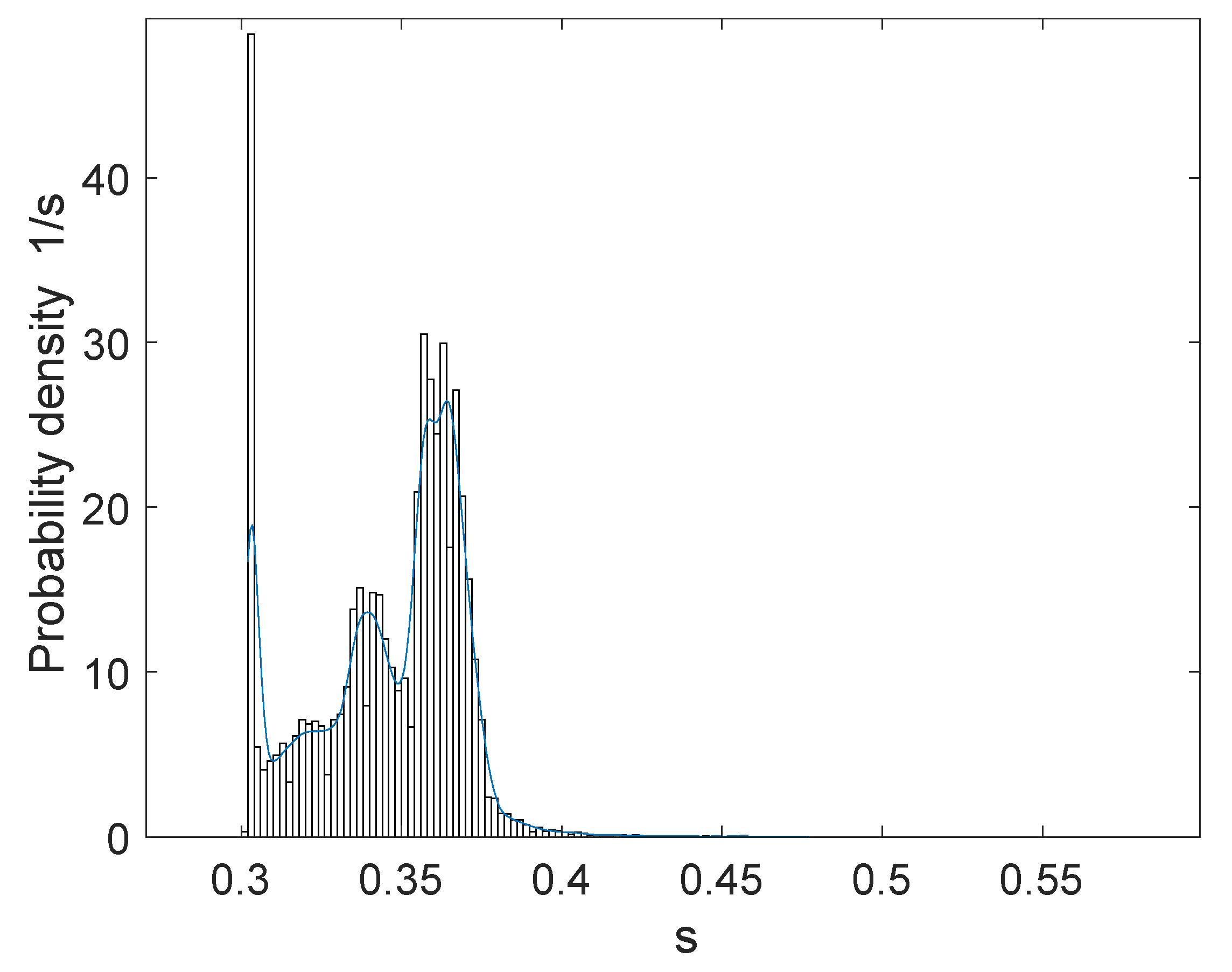
The empirical distribution of the cycle time $T_S$ (Figure 9) is different from the normal or Poisson and is polymodal. In accordance with the functioning algorithm, each of the modes corresponds to a typical processing cycle for a particular type of data.

For this sample, the maximum delay was estimated using service curves 7 and 11. The results for sample size $L~{10}^3$ are shown in

Table 1. The experimental delay calculation results for I&C system component Z.

Parameter	Value
$D_x$	0.37
$p\left(D_x\right)$	$~1$
$D_{}$	5.1
$p\left(D_{}\right)$	$~1$
$D/D_x$	4.9
$D^{\prime }$	0.32
$p\left(D^{\prime }\right)$	0.87
$D^{\prime }/D_x$	0.3

.

In the experiment, we measured the network delay $T_E$ using the tcpdump utility from the Linux OS. The round-trip time (RTT) of a TCP packet was measured, i.e., the time elapsed from the moment the S component sent packet until the confirmation (ACK, [25]) receipt from the Z component. The typical round trip time of a packet is tens of microseconds and the maximum transit time of network packets is $~{10}^3$ times less than the processing time of information in cycles. The characteristics of the process of transferring data between other components of the system are similar. The condition that $T_E\ll T_s$ allows using the simplified Formula (18) to calculate the service curve.

In the course of measurements on a real I&C system, we verified that the empirical distributions obtained from measurements (Figure 9) have a heavy tail. The check was carried out using the algorithm for recognizing distributions with heavy tails [26], which, on the author’s tests, showed better results than tests based on the Kolmogorov–Smirnov criteria.

The test showed that a real system of distribution of time delays, both in the network components and in the components that process information, belong to a heavy-tailed distribution.

8. Results and Discussion

The paper considers estimating the temporal characteristics of digital I&C control systems (CS) during the system’s validation. CS technical requirements often include constraints on data processing and communication delays. The constraints can be imposed on both average and maximum (absolute) values. They can be expressed either as statistical constraints with confidence intervals or as limiting absolute values [27].

Estimating a random variable from a sample is a classical problem of statistics. It is well described in the literature (see, for example, [28]). However, the interpretation of the measured characteristics of the digital I&C system with a presumption that the probability law of the values is close to normal may lead to incorrect conclusions. Let us formulate the main problems.

The procedure of technical requirements validation during tests is mainly based on calculating the sample mean and sample variance (for example, [1]). If a random variable has a finite expectation value and variance, the sample mean is an unbiased consistent estimation of the theoretical mean and does not depend on the type of distribution. A known disadvantage of this method is its low robustness in extraneous outliers in the sample [28]. However, sample variance, both biased and unbiased, is a consistent estimate of the theoretical variance of a quantity.

In practice, when interpreting the obtained estimates of the mean and variance, it is implicitly assumed that the time delays are distributed according to the normal law and intuitively transfer the estimates of the confidence intervals for the normally distributed quantity to the case of time delays in control systems. Indeed, if a random variable has a normal distribution then, having a sample mean and variance, it is easy to estimate the confidence interval for the parameter being confirmed. However, the probability function of the delay in the CS is generally not normal.

The physical nature of the measured value (time) imposes restrictions on the probability distribution function. At least, it is bounded on the left. If the technical requirements specify the maximum absolute value (for example, “the signal transit time between the CS components should not exceed a certain value”) this form of the requirement implies that the random variable has a distribution function that is also bounded from the right. So, the absolute restrictions mean that the distribution function is not initially, in the strict sense, a distribution function of a normal random variable.

Our study of a real CS encountered that the distributions of the data processing and communication delays significantly differ from the normal, often have polymodal nature, and belong to heavy-tailed distributions. In a general sense, to estimate the probability of a random variable exceeding a particular value, one can use Samuelson’s–Chebyshev’s inequality. However, it gives a very rough estimate.

The paper considers a non-statistical approach for delay calculation in CS based on the network calculus method. The network calculus method is not entirely new, but it is still not well understood by testing specialists. When applying it to the analysis of computer systems, it is necessary to take into account some of the peculiarities of the method. Thus, the input data about the system, which are necessary for the calculation using the network calculus method, in the general case, are not specified as “logbook parameters” of the system. For example, such input data for the method are flow envelopes, service curves, scaling functions in the case of an uneven data flow, etc. are a priori unknown. There is also the lack of transparency in corresponding the network calculus results with classical (statistical) methods. The technical difficulties of the method are known, and various approaches to partially resolve them have been developed, for example, [8,9,10,11,19,29]. However, these solutions also require initial data about the system, which are absent or poorly formalized in practice.

Within the frames of network calculus, we proposed a mathematical model for the description of computer systems with cyclic data processing algorithms that are common in CSs. The model allows one to take into account data heterogeneity and significantly simplifies delay calculations if the major delay is due to the data processing.

We got solutions for two subproblems. First, we proved a necessary condition of the minimum service curve existence that allows estimating the curve from data flows. Second, we performed simulations of the correspondence of network calculus and statistical results.

In particular, it is shown that the closest correspondence between the statistically calculated maximum delay and the calculation of the maximum delay by the Network Calculus method is obtained when the data distribution in the sample has single large outliers, which is typical for heavy-tailed distributions. It is assumed that the maximum delay is related to the probability of a rare event, a sequential arrival of a significant amount of data with low server performance for a minimum service curve.

The developed methods are verified on simulating examples and successfully applied to the real I&C system.

We have not managed to formulate a sufficient condition on the minimum service curve. It is possible that a sufficient condition for a general case does not exist. However, we hope to obtain a sufficient condition for the particular case of realizable service curves.