
Transient Dynamic Analysis of Unconstrained Layer Damping Beams Characterized by a Fractional Derivative Model


Abstract
:1. Introduction
2. Homogenized Model for an FLD Beam
2.1. Homogenized Finite Element Formulation
2.2. Numerical Integration
3. Description of the Model
4. Numerical Analysis
- Amplitude ratio between the first relative maximum and the first relative minimum, . This parameter illustrates the initial intensity of the response. The higher this value, the larger the system oscillates at first, and therefore, the lower the value, the higher it is the attenuation of the vibration. This variable is important, for example, in human comfort applications.
- Amplitude ratio between the first relative maximum and the stationary response (which is always normalized to 1), . The higher this amplitude, the lesser the vibration attenuation present into the beam.
- Number of cycles to reduce the vibration. This is considered when the difference between a relative maximum and the consecutive relative minimum is the 5% of the mean value between them, i.e., the next equation is satisfied,for practical applications, it is desired a low value in the number of cycles in order to get a quicker vibration attenuation.
- Time ratio : is the time at which the system reaches the stationary value with a tolerance of and is the required time to perform the cycles previously mentioned. This ratio should be as low as possible in order to get a faster time response.
4.1. Analysis of the Influence of the Viscoelastic Material Parameters
4.1.1. Initial Amplitude Ratio Influence
4.1.2. First Maximum and Stationary Amplitude Ratio Influence
4.1.3. Number of Cycles Influence
4.1.4. Time Ratio Influence
4.2. Analysis of the Influence of the Viscoelastic Layer Thickness
4.3. Examples of Parameter Combination
5. Conclusions
Author Contributions
Funding
Institutional Review Board Statement
Informed Consent Statement
Data Availability Statement
Conflicts of Interest
References
- Rao, M.D. Recent Applications of Viscoelastic Damping for Noise Control in Automobiles and Commercial Airplanes. J. Sound Vib. 2003, 262, 457–474. [Google Scholar] [CrossRef]
- Chakraborty, B.; Ratna, D. Polymers for Vibration Damping Applications, 1st ed.; Elsevier: Amsterdam, The Netherlands, 2020. [Google Scholar]
- Sun, C.T.; Lu, Y.P. Vibration Damping of Structural Elements, 1st ed.; Prentice Hall: Englewood Cliffs, NJ, USA, 1995. [Google Scholar]
- Nashif, A.D.; Jones, D.I.; Henderson, J.P. Vibration Damping, 1st ed.; John Wiley & Sons: New York, NY, USA, 1985. [Google Scholar]
- Elejabarrieta, M.J.; Cortés, F.; Martínez, M. Viscoelastic Surface Treatments for Passive Control of Structural Vibration, 1st ed.; Nova Science Publishers: New York, NY, USA, 2011. [Google Scholar]
- Zheng, H.; Cai, C.; Tan, X.M. Optimization of partial constrained layer damping treatment for vibrational energy minimization of vibrating beams. Comput. Struct. 2004, 82, 2493–2507. [Google Scholar] [CrossRef]
- Irazu, L.; Elejabarrieta, M.J. The influence of viscoelastic film thickness on the dynamic characteristics of thin sandwich structures. Compos. Struct. 2015, 134, 421–428. [Google Scholar] [CrossRef]
- Lall, A.K.; Nakra, B.C.; Asnani, N.T. Optimum design of viscoelastically damped sandwich panels. Eng. Optim. 1983, 6, 197–205. [Google Scholar] [CrossRef]
- Irazu, L.; Elejabarrieta, M.J. The effect of the viscoelastic film and metallic skin on the dynamic properties of thin sandwich structures. Compos. Struct. 2017, 176, 407–419. [Google Scholar] [CrossRef]
- Zarraga, O.; Sarría, I.; García-Barruetabeña, J.; Cortés, F. Homogenised formulation for plates with thick constrained viscoelastic core. Comput. Struct. 2020, 229, 106185. [Google Scholar] [CrossRef]
- Sun, W.; Yan, X.; Gao, F. Analysis of Frequency-Domain Vibration Response of Thin Plate Attached with Viscoelastic Free Layer Damping. Mech. Based Des. Struct. Mach. 2018, 46, 209–224. [Google Scholar] [CrossRef]
- Adolfsson, K.; Enelund, M.; Olsson, P. On the fractional order model of viscoelasticity. Mech. Time-Depend. Mater. 2005, 9, 15–34. [Google Scholar] [CrossRef]
- Podlubny, I. Fractional Differential Equations, 1st ed.; Academic Press: Cambridge, NY, USA, 1998. [Google Scholar]
- Jannelli, A. Numerical solutions of fractional differential equations arising in engineering sciences. Mathematics 2020, 8, 215. [Google Scholar] [CrossRef] [Green Version]
- Miller, K.; Ross, B. An Introduction to the Fractional Calculus and Fractional Differential Equations, 1st ed.; John Wiley & Sons: New York, NY, USA, 1993; pp. 19–93. [Google Scholar]
- Bagley, R.L.; Torvik, P.J. Fractional calculus—A different approach to the analysis of viscoelastically damped structures. AIAA J. 1983, 21, 741–748. [Google Scholar] [CrossRef]
- Cortés, F.; Elejabarrieta, M.J. Finite element analysis of the seismic response of damped structural systems including fractional derivative models. J. Vib. Acoust. Trans. ASME 2014, 136, 050901. [Google Scholar] [CrossRef]
- Hinze, M.; Schmidt, A.; Leine, R.I. The direct method of lyapunov for nonlinear dynamical systems with fractional damping. Nonlinear Dyn. 2020, 102, 2017–2037. [Google Scholar] [CrossRef]
- Zarraga, O.; Sarría, I.; García-Barruetabeña, J.; Cortés, F. An analysis of the dynamical behaviour of systems with fractional damping for mechanical engineering applications. Symmetry 2019, 11, 1499. [Google Scholar] [CrossRef] [Green Version]
- Zarraga, O.; Sarría, I.; García-Barruetabeña, J.; Elejabarrieta, M.J.; Cortés, F. General homogenised formulation for thick viscoelastic layered structures for finite element applications. Mathematics 2020, 8, 714. [Google Scholar] [CrossRef]
- Praharaj, R.K.; Datta, N. On the transient response of plates on fractionally damped viscoelastic foundation. Comput. Appl. Math. 2020, 39, 256. [Google Scholar] [CrossRef]
- Al-Huniti, N.; Al-Faqs, F.; Abu Zaid, O. Finite element dynamic analysis of laminated viscoelastic structures. Appl. Compos. Mater. 2010, 17, 405–414. [Google Scholar] [CrossRef]
- Kiasat, M.S.; Zamani, H.A.; Aghdam, M.M. On the transient response of viscoelastic beams and plates on viscoelastic medium. Int. J. Mech. Sci. 2014, 83, 133–145. [Google Scholar] [CrossRef]
- Shafei, E.; Faroughi, S.; Rabczuk, T. Nonlinear transient vibration of viscoelastic plates: A NURBS-Based isogeometric HSDT approach. Comput. Math. Appl. 2021, 84, 1–15. [Google Scholar] [CrossRef]
- Cunha-Filho, A.G.; Briend, Y.; de Lima, A.M.G.; Donadon, M.V. A new and efficient constitutive model based on fractional time derivatives for transient analyses of viscoelastic systems. Mech. Syst. Signal Process. 2021, 146, 107042. [Google Scholar] [CrossRef]
- Sarría, I.; García-Barruetabeña, J.; Cortés, F.; Mateos, M. Dynamic Analysis of nonlinear structural systems by means of fractional calculus. DYNA Ing. Ind. 2015, 90, 54–60. [Google Scholar] [CrossRef] [Green Version]
- Zarraga, O.; Sarría, I.; García-Barruetabeña, J.; Cortés, F. Dynamic analysis of plates with thick unconstrained layer damping. Eng. Struct. 2019, 201, 109809. [Google Scholar] [CrossRef]
- Cortés, F.; Elejabarrieta, M.J. Homogenised finite element for transient dynamic analysis of unconstrained layer damping beams involving fractional derivative models. Comput. Mech. 2007, 40, 313–324. [Google Scholar] [CrossRef]
- Gere, J.M.; Timoshenko, S. Mechanics of Materials, 4th ed.; PWS Publishing Company: Boston, MA, USA, 1996. [Google Scholar]
- Inman, D.J. Engineering Vibration, 4th ed.; Prentice Hall: Englewood Cliffs, NJ, USA, 1996. [Google Scholar]
- Megson, T. Structural and Stress Analysis, 1st ed.; Butterworth-Heinemann: Bodmin, UK, 1996. [Google Scholar]
- Universidad de Vigo. Available online: http://www.dma.uvigo.es/files/cursos/mef/teoria.pdf (accessed on 21 April 2021).
- Bathe, K.-J. Finite Element Procedures, 1st ed.; Prentice Hall: Englewood Cliffs, NJ, USA, 1996. [Google Scholar]
- Cortés, F.; Elejabarrieta, M.J. Finite element formulations for transient dynamic analysis in structural systems with viscoelastic treatments containing fractional derivative models. Int. J. Numer. Methods Eng. 2007, 69, 2173–2195. [Google Scholar] [CrossRef]
- Jones, D.I. Handbook of Viscoelastic Vibration Damping, 1st ed.; John Wiley & Sons: New York, NY, USA, 2001. [Google Scholar]
- García-Barruetabeña, J.; Cortés, F.; Manuel Abete, J. Influence of nonviscous modes on transient response of lumped parameter systems with exponential damping. J. Vib. Acoust. 2011, 133, 064502. [Google Scholar] [CrossRef]
 ) and viscoelastic (
  ) material distribution in both FLD configurations: (a) Asymmetrical configuration; (b) Symmetrical configuration.
) and viscoelastic ( ) material distribution in both FLD configurations: (a) Asymmetrical configuration; (b) Symmetrical configuration.
) material distribution in both FLD configurations: (a) Asymmetrical configuration; (b) Symmetrical configuration.
) and viscoelastic ( ) material distribution in both FLD configurations: (a) Asymmetrical configuration; (b) Symmetrical configuration.
 ) represent the interval of the stationary response, which is always 1 according to the definition of the displacement ratio .
) represent the interval of the stationary response, which is always 1 according to the definition of the displacement ratio .
) represent the interval of the stationary response, which is always 1 according to the definition of the displacement ratio .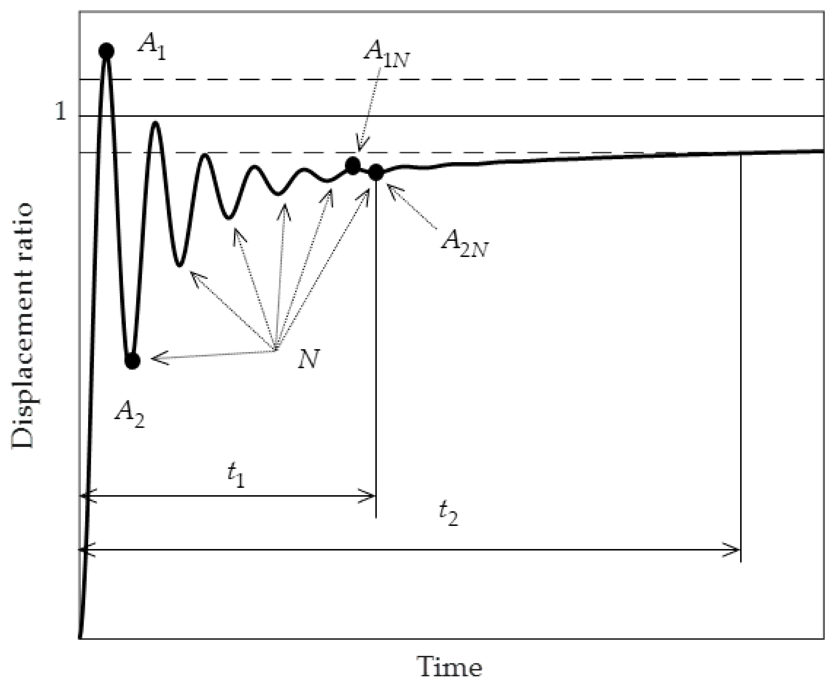
 ) and symmetrical (
  ) configurations. In order: (a) Relaxed modulus ; (b) Unrelaxed modulus ; (c) Fractional parameter ; (d) Fractional parameter ; (e) Relaxation time .
) and symmetrical ( ) configurations. In order: (a) Relaxed modulus ; (b) Unrelaxed modulus ; (c) Fractional parameter ; (d) Fractional parameter ; (e) Relaxation time .
) configurations. In order: (a) Relaxed modulus ; (b) Unrelaxed modulus ; (c) Fractional parameter ; (d) Fractional parameter ; (e) Relaxation time .
) and symmetrical ( ) configurations. In order: (a) Relaxed modulus ; (b) Unrelaxed modulus ; (c) Fractional parameter ; (d) Fractional parameter ; (e) Relaxation time .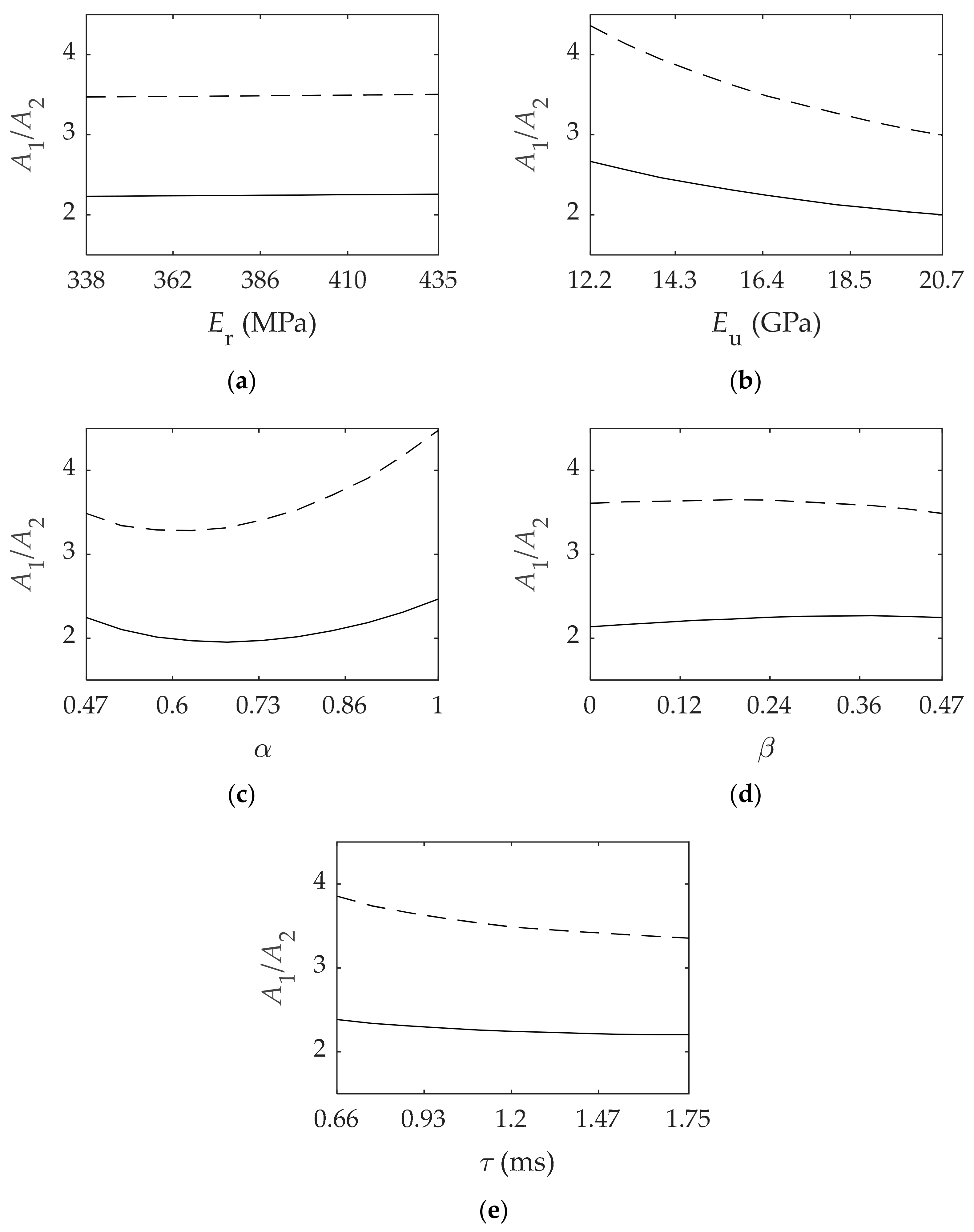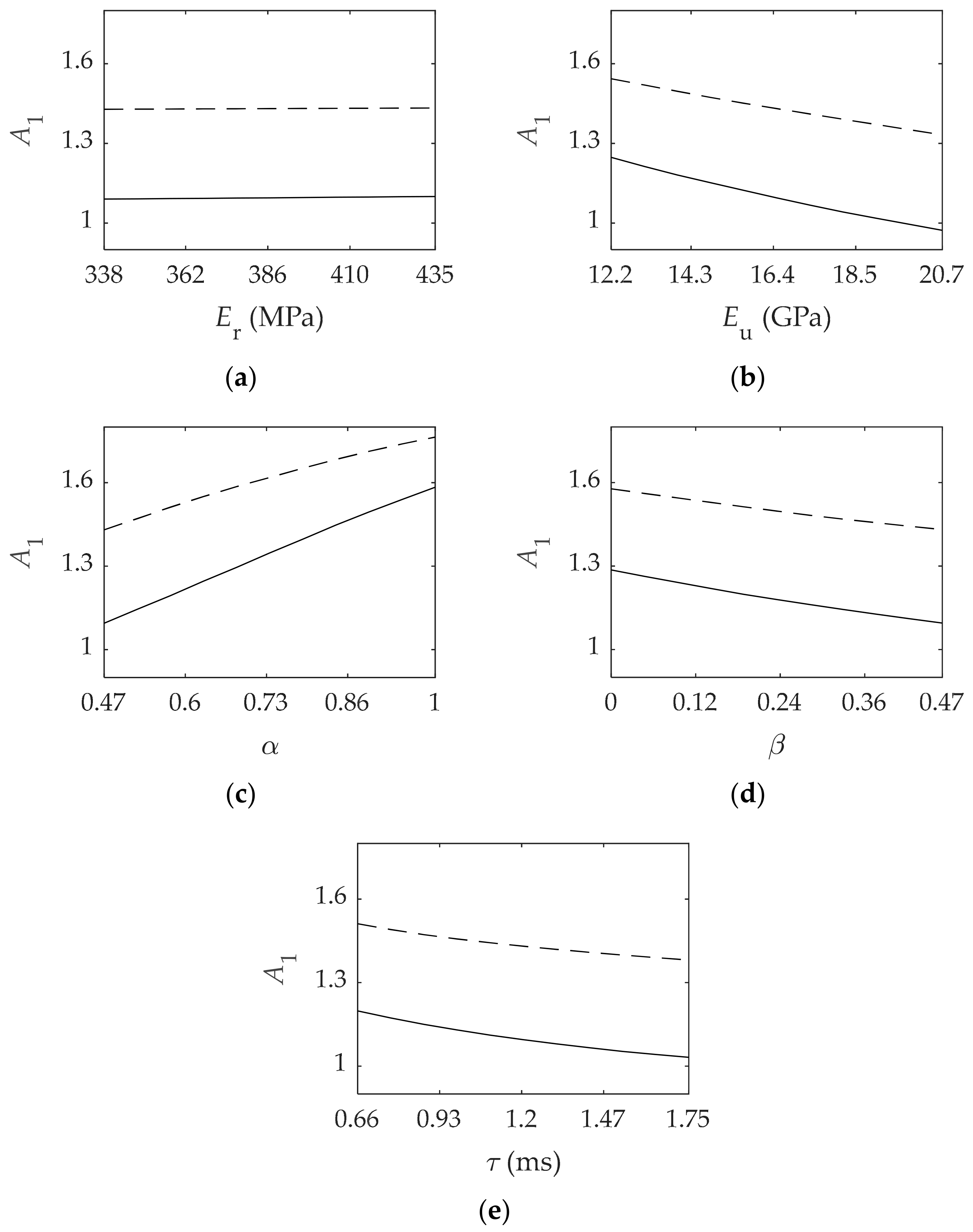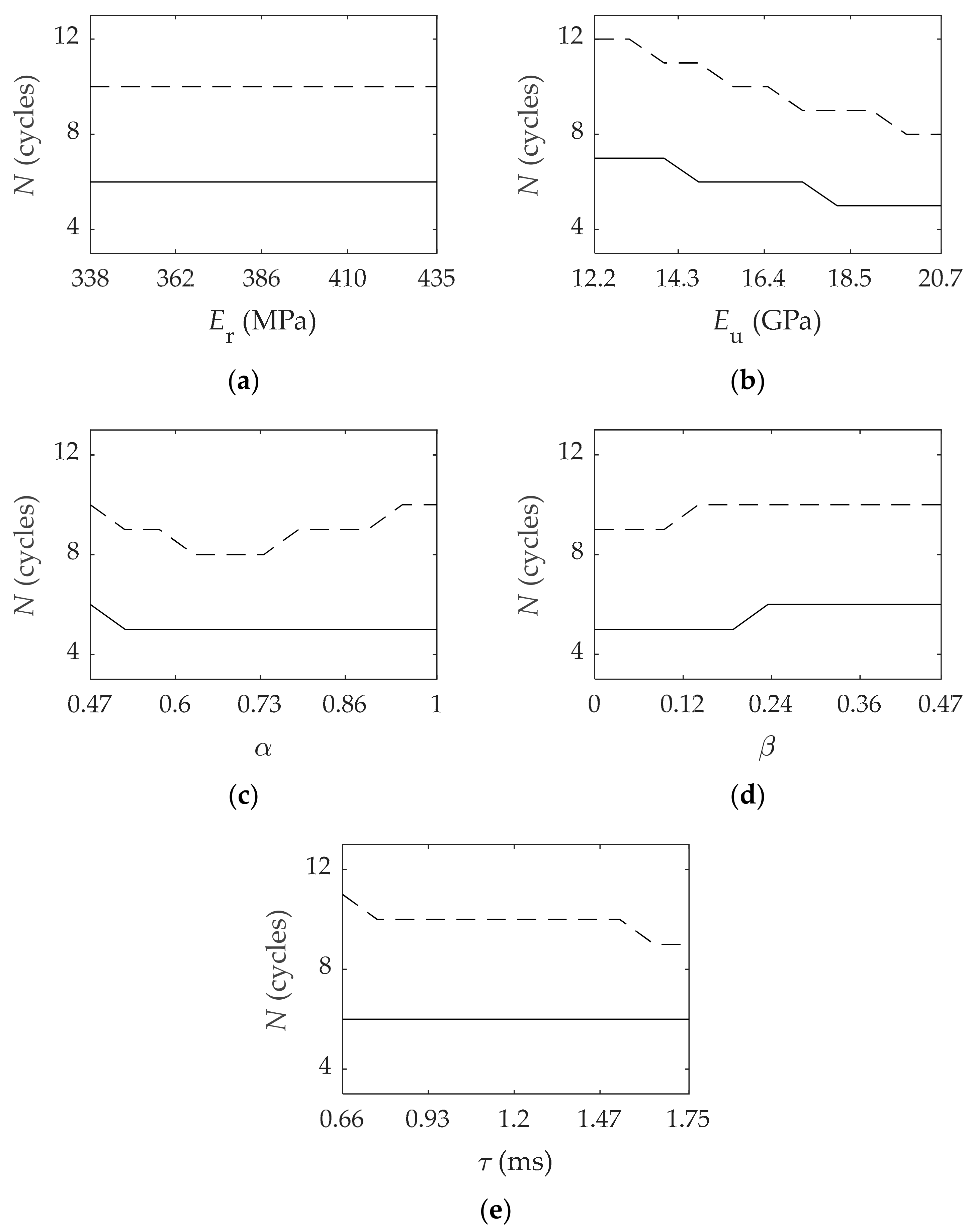
 ) represents point of equilibrium changing over time and the two horizontal dashed lines (
  ) represent the interval of the stationary response.
) represents point of equilibrium changing over time and the two horizontal dashed lines ( ) represent the interval of the stationary response.
) represent the interval of the stationary response.
) represents point of equilibrium changing over time and the two horizontal dashed lines ( ) represent the interval of the stationary response.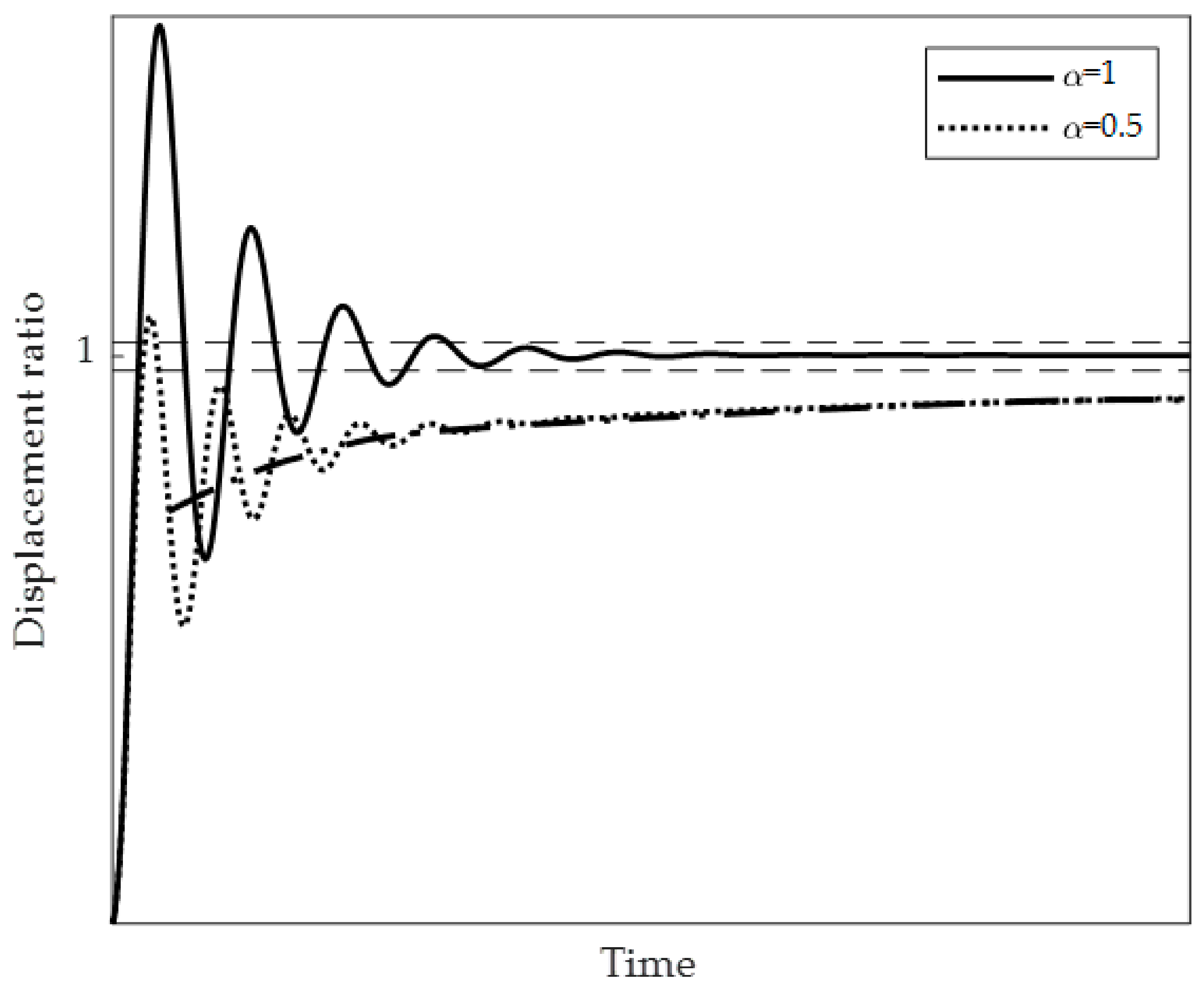
 ) and symmetrical (
  ) configurations on: (a) Ratio between the first relative maximum and the first relative minimum ; (b) Ratio between the amplitude of the first maximum and the stationary response ; (c) Number of cycles ; (d) Time ratio .
) and symmetrical ( ) configurations on: (a) Ratio between the first relative maximum and the first relative minimum ; (b) Ratio between the amplitude of the first maximum and the stationary response ; (c) Number of cycles ; (d) Time ratio .
) configurations on: (a) Ratio between the first relative maximum and the first relative minimum ; (b) Ratio between the amplitude of the first maximum and the stationary response ; (c) Number of cycles ; (d) Time ratio .
) and symmetrical ( ) configurations on: (a) Ratio between the first relative maximum and the first relative minimum ; (b) Ratio between the amplitude of the first maximum and the stationary response ; (c) Number of cycles ; (d) Time ratio .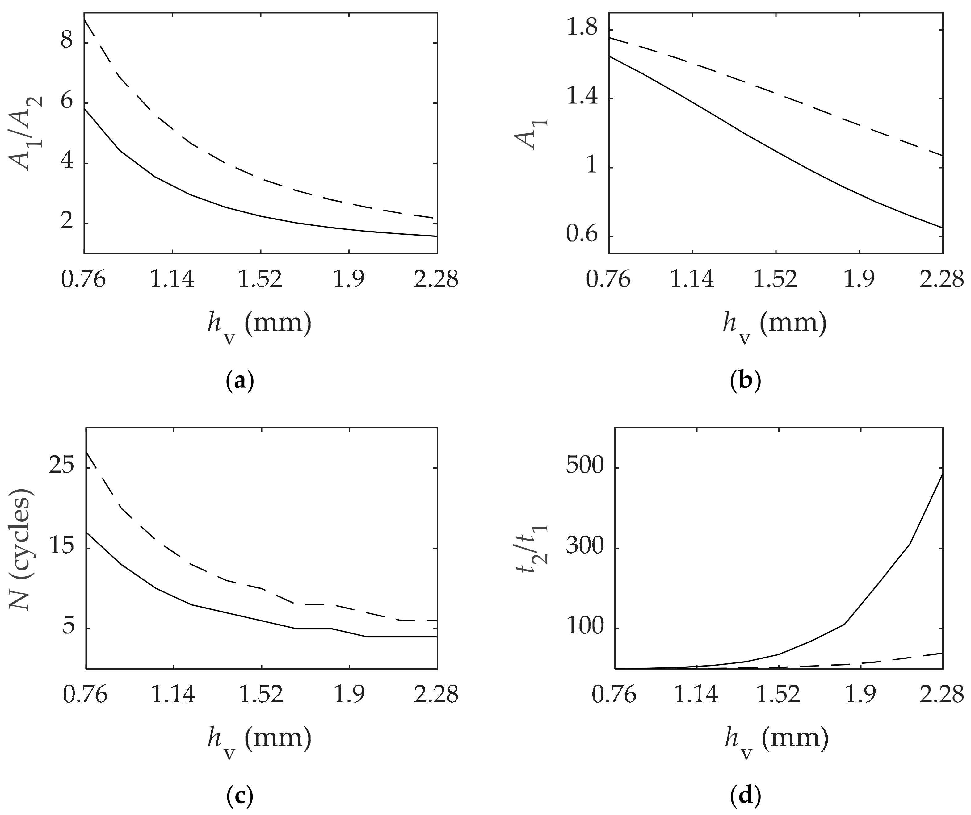
 ) represent the interval with regard to the normalized displacement ratio at the stationary value.
) represent the interval with regard to the normalized displacement ratio at the stationary value.
) represent the interval with regard to the normalized displacement ratio at the stationary value.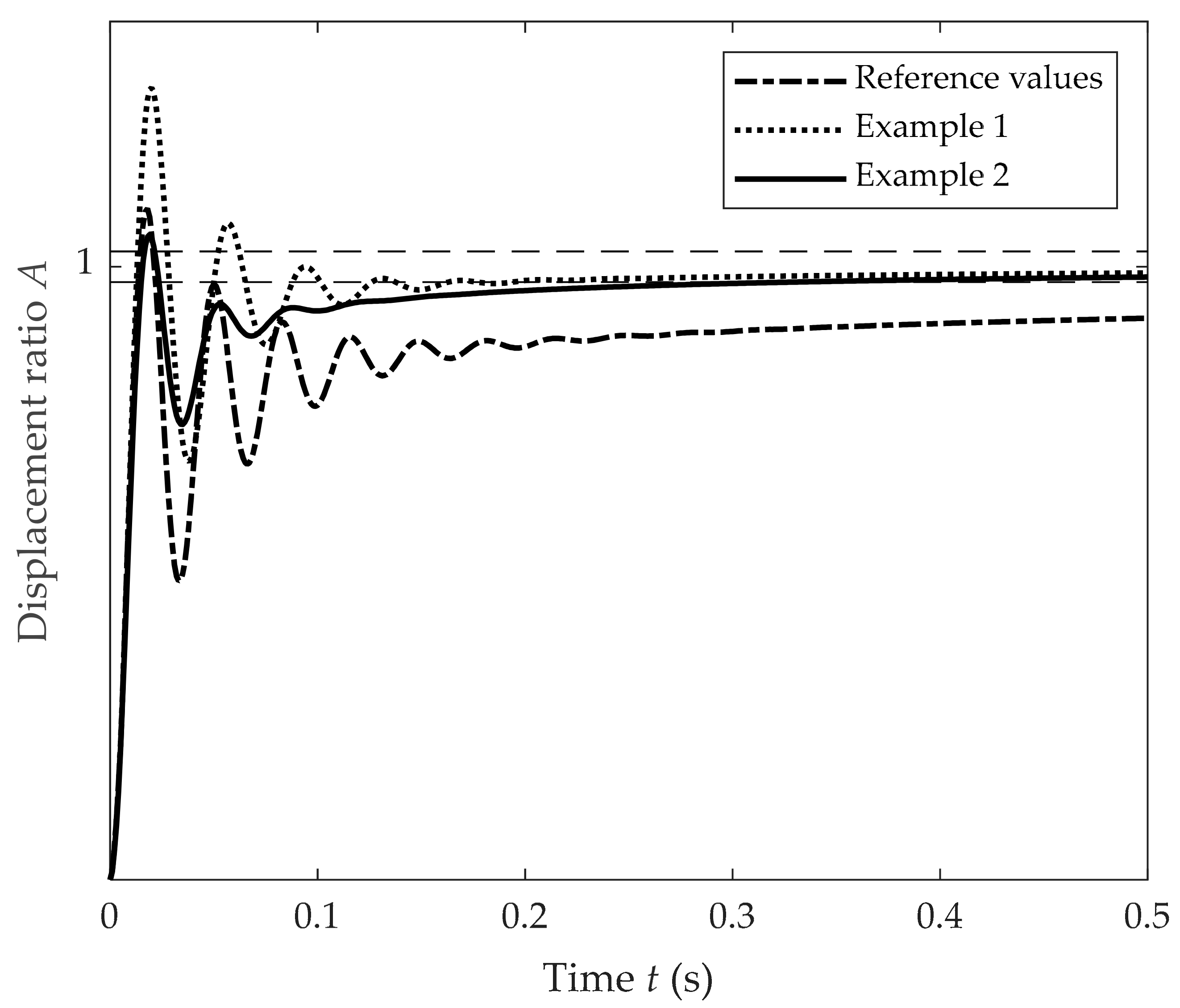

| Parameter | Value |
|---|---|
| 180 | |
| 9.85 | |
| 1.05 | |
| 7782 | |
| 176.2 |
| Parameter | Reference | Interval | |
|---|---|---|---|
| Minimum | Maximum | ||
| 386.5 | 338.2 | 434.9 | |
| 16.49 | 12.26 | 20.71 | |
| 0.47 | 0.47 | 1 | |
| 0.47 | 0 | 0.47 | |
| 1.205 | 0.660 | 1.750 | |
| 1.52 | 0.76 | 2.28 | |
| Parameter | Reference Values | Example 1 Values | Example 2 Values |
|---|---|---|---|
| 386.6 | 386.6 | 386.6 | |
| 16.49 | 17.30 | 17.30 | |
| 0.47 | 0.682 | 0.682 | |
| 0.47 | 0.3 | 0.3 | |
| 1.2 | 1.4 | 1.4 | |
| 1.52 | 1.52 | 1.9 |
| Case | ||||||
|---|---|---|---|---|---|---|
| Reference | 2.24 | 1.10 | 6 | 0.195 s | 7.01 s | 36.0 |
| Example 1 | 1.89 | 1.29 | 4 | 0.149 s | 0.194 s | 1.30 |
| Example 2 | 1.41 | 1.05 | 3 | 0.100 s | 0.329 s | 3.29 |
Publisher’s Note: MDPI stays neutral with regard to jurisdictional claims in published maps and institutional affiliations. |
© 2021 by the authors. Licensee MDPI, Basel, Switzerland. This article is an open access article distributed under the terms and conditions of the Creative Commons Attribution (CC BY) license (https://creativecommons.org/licenses/by/4.0/).
Share and Cite
Brun, M.; Cortés, F.; Elejabarrieta, M.J. Transient Dynamic Analysis of Unconstrained Layer Damping Beams Characterized by a Fractional Derivative Model. Mathematics 2021, 9, 1731. https://doi.org/10.3390/math9151731
Brun M, Cortés F, Elejabarrieta MJ. Transient Dynamic Analysis of Unconstrained Layer Damping Beams Characterized by a Fractional Derivative Model. Mathematics. 2021; 9(15):1731. https://doi.org/10.3390/math9151731
Chicago/Turabian StyleBrun, Mikel, Fernando Cortés, and María Jesús Elejabarrieta. 2021. "Transient Dynamic Analysis of Unconstrained Layer Damping Beams Characterized by a Fractional Derivative Model" Mathematics 9, no. 15: 1731. https://doi.org/10.3390/math9151731
APA StyleBrun, M., Cortés, F., & Elejabarrieta, M. J. (2021). Transient Dynamic Analysis of Unconstrained Layer Damping Beams Characterized by a Fractional Derivative Model. Mathematics, 9(15), 1731. https://doi.org/10.3390/math9151731