Theoretical Efficiency Study of Output Lubricant Flow Rate Regulating Principle on the Example of a Two-Row Aerostatic Journal Bearing with Longitudinal Microgrooves and a System of External Combined Throttling

Abstract

Due to their vanishingly low air friction, high wear resistance, and environmental friendliness, aerostatic bearings are used in machines, machine tools, and devices that require high accuracy of micro-movement and positioning. The characteristic disadvantages of aerostatic bearings are low load capacity, high compliance and an increased tendency for instability. In radial bearings, it is possible to use longitudinal microgrooves, which practically exclude circumferential air leakage, and contributes to a significant increase in load-bearing capacity. To reduce compliance to zero and negative values, inlet diaphragm and elastic airflow regulators are used. Active flow compensation is inextricably linked to the problem of ensuring the stability of bearings due to the presence of relatively large volumes of gas in the regulator, which have a destabilizing effect. This problem was solved by using an external combined throttling system. Bearings with input flow regulators have a number of disadvantages-they are very energy-intensive and have an insufficiently stable load capacity. A more promising way to reduce compliance is the use of displacement compensators for the movable element. Such bearings also allow for a decrease in compliance to zero and negative values, which makes it possible to use them not only as supports, but also as active deformation compensators of the technological system of machine tools in order to reduce the time and increase the accuracy of metalworking. The new idea of using active flow compensators is to regulate the flow rate not at the inlet, but at the outlet of the air flow. This design has the energy efficiency that is inherent to a conventional bearing, but the regulation of the lubricant output flow allows the compliance to be reduced to zero and negative values. This article discusses the results of a theoretical study of the static and dynamic characteristics of a two-row radial aerostatic bearing with longitudinal microgrooves and an output flow regulator. Mathematical modeling and theoretical study of stationary modes have been carried out. Formulas for determining static compliance and load capacity are obtained. Iterative finite-difference methods for determining the dynamic characteristics of a structure are proposed. The calculation of dynamic quality criteria was carried out on the basis of the method of rational interpolation of the bearing transfer function, as a system with distributed parameters, developed by the authors. It was found that the volumes of the microgrooves do not have a noticeable effect on the bearing dynamics. It is shown that, in this design, the external combined throttling system is an effective means of maintaining stability and high dynamic quality of the design operating in the modes of low, zero and negative compliance.

1. Introduction

Due to the vanishingly low friction in the air, high wear resistance, and environmental friendliness, aerostatic bearings are used in machines, in particular, in machine tools, which are devices that require high accuracy of micro-movement and positioning [1,2,3,4,5,6,7,8]. In mechanical engineering, aerostatic bearings are used in the spindle assemblies of metal-cutting machine tools [9,10,11,12].

Typical disadvantages of aerostatic bearings are low load-bearing capacity, high compliance (low stiffness) and increased tendency to instability. The first two drawbacks are explained by the limited injection pressure, while the latter is determined by the high air compressibility even in microvolumes [13,14]. To improve the static characteristics of radial bearings, two-row feeding systems and longitudinal microgrooves made in the inter-row zone are used, which practically exclude circumferential air leakage, and contributes to a significant increase in the load capacity [15,16,17]. To reduce compliance, aerostatic bearings with active air flow compensation are used, where inlet flow compensators; membrane regulators of the nozzle-damper type with throttles in the form of diaphragms with sharp edges and in the form of flat slots [18,19,20,21,22] or Laub elastic orifices, are used [23,24,25]. The use of inlet membrane or elastic regulators makes it possible to reduce the static compliance to zero and even negative values (in the latter case, the increments of the load and the bearing gap have the same signs).

The technical problem of implementing the principle of active flow compensation is inextricably linked with the problem of ensuring the stability of bearings due to the presence of relatively large volumes of gas in the regulator, which have a destabilizing effect. This problem found a solution in the form of using an system of external combined throttling (SECT) containing the main throttling resistance, additional damping resistance and a flow-through air resonator chamber located between them, the optimal volume of which contributes to a drastic improvement in dynamic characteristics [26,27]. Diaphragms or elastic regulators act as the main resistance, and for damping resistance, annular diaphragms proved to be the best, the optimal resistance of which should be 5–15% of the total resistance of the SECT [19,28,29]. Such ratios of SECT resistances, in combination with the optimal volume of the throttle chamber, provide the best dynamics quality during the operation of bearings at almost any compliance, including zero and negative.

Bearings with an inlet diaphragm or resilient regulators have at least three disadvantages. The first is that they are too energy intensive due to the need to significantly increase the lubricant consumption using the input regulators to reduce compliance. In addition, such bearings have an insufficiently stable characteristic of load capacity, where low compliance is provided only in a narrow range of loads (this is especially characteristic of open thrust bearings with diaphragm regulators) [24,25]. Finally, the third drawback arises from the first-too large a gain of the regulators has an increased negative effect on the bearing dynamics, where it is difficult to ensure low compliance even in the presence of the optimal dynamics of the SECT [25].

A more effective solution to reduce compliance is the use of compensators for displacement of the movable element (shaft) [18,19,20]. Such bearings also allow for a decrease in compliance to zero and negative values, which, like designs with membrane and elastic regulators, allows them to be used not only as supports, but also as active deformation compensators of the technological system of machine tools in order to reduce time and increase the accuracy of metalworking. The SECT provides a significant decrease in compliance and guaranteed stability [27].

The new idea of using active flow compensators is to regulate the flow rate not at the inlet, but at the outlet of the air flow. Its essence lies in the fact that in the SECT inlet, ordinary simple diaphragms are installed instead of regulators, and the regulator itself is located in the bearing gap at the air outlet from the gap to actively limit the flow rate in order to reduce compliance. The design should have the energy efficiency of a conventional bearing, but in contrast, control of the lubricant output should help reduce compliance.

This article discusses the results of a theoretical study of the static and dynamic characteristics of a two-row radial aerostatic bearing with a SECT, longitudinal microgrooves and an output flow regulator.

2. Description of the Bearing Design and the Principle of Its Operation

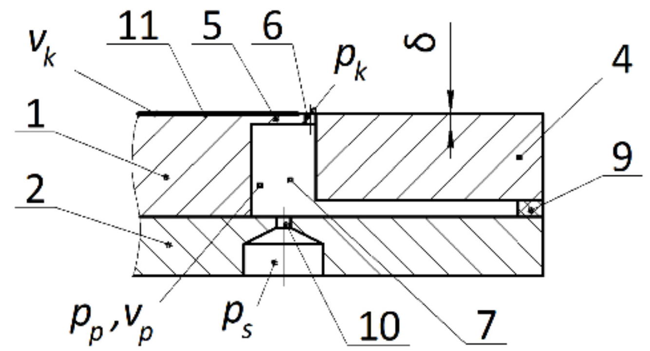
Figure 1 shows the design of the bearing. It contains a support sleeve, 1, installed in the housing, 2. Between the surface of the sleeve, 1, and the shaft, 3, a gas bearing gap is formed, which ensures the operation of the bearing.

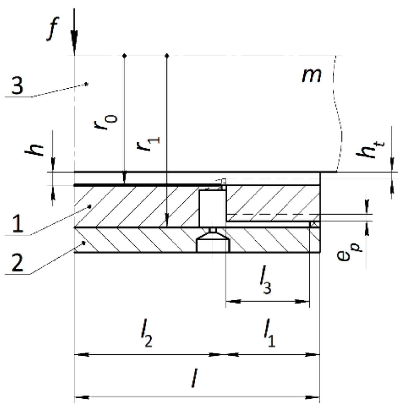
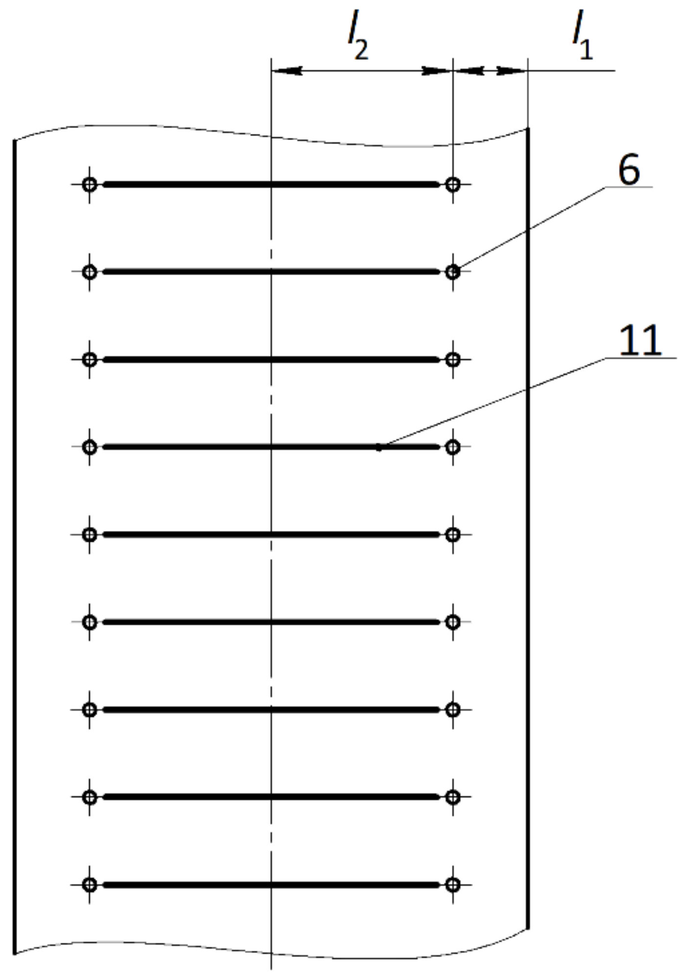
The sleeve, 1, contains a movable part, 4 (Figure 2), connected to the main part by means of a thin membrane, 5. The membrane has throttling holes, 6, connecting the cavities, 7, with the bearing gas gap.

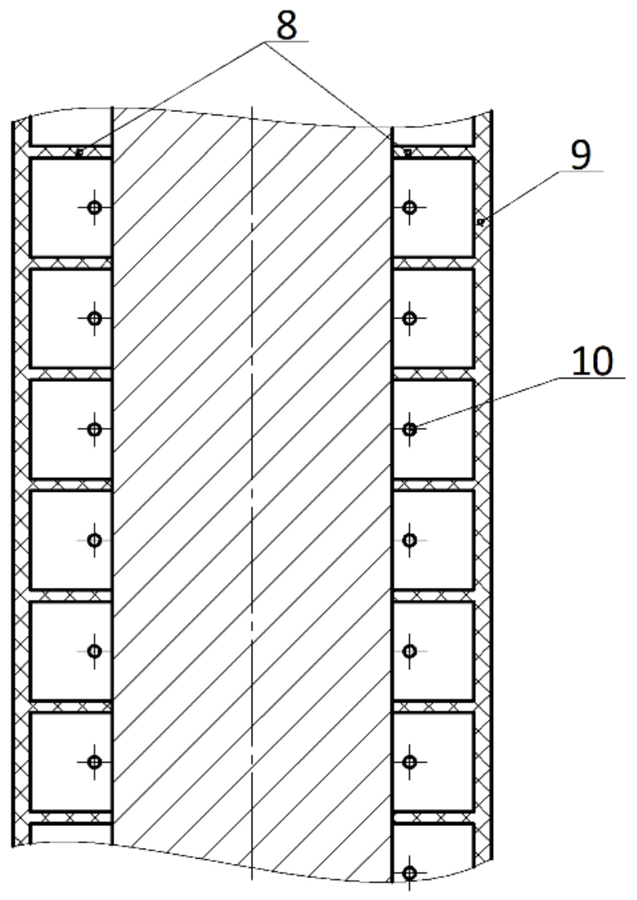
These cavities are separated by partitions, 8, made of elastic material, as shown in the unfolded drawing (Figure 3).

The same elastic material is used to seal the cavities, 7, by means of seals, 9. Each cavity, 7, is connected to an external source of lubricant injection by means of the main throttles, 10. On the bearing surface of the support sleeve, 1, fine microgrooves, 11, are made, starting at a small distance from the holes, 7, and located in parallel on the longitudinal axis, as shown in Figure 4.

When the bearing is operating, gas from an external injection source under pressure p_s enters through the main throttles, 10, into the cavities, 7, and then through the damping throttles, 6, into the bearing gas gap, after which it flows out into the environment. With a radial displacement of the shaft, 3, the gap h in the loaded region decreases, which leads to an increase in the resistance to gas flow in the bearing gap. As a result, the pressures p_k and p_p increase. Under the influence of the increased pressure in the region l₃, the movable annular part, 4, is displaced towards the shaft, 3, by a distance e_p, as a result, the gap at the exit from the bearing layer decreases to the value h_t. This leads to an additional increase in pressure p_k in the loaded region. On the opposite side of the bearing in the unloaded area, due to effects opposite to those described, the pressure p_k decreases. These changes in pressure p_k lead to a decrease in bearing compliance.

3. Mathematical Modeling of the Bearing Static State at Small Deviations of the Moving Elements from the Central Equilibrium Position

The simplest theoretical substantiation of the fundamental possibility of reducing the bearing compliance by limiting the flow rate of the lubricant output flow can be carried out by performing a study of small radial deviations of the bearing’s moving elements, which are caused by a small effect on the shaft, 3, from the external load f. When simulating small deviations in a stationary mode, we will assume that the parallelism of the axes of the housing, 2, shaft, 3, and bushing, 1, is preserved. We also assume that the number of annular diaphragms in each row is large enough, which makes it possible to calculate the characteristics of the bearing by the method of continuous pressurization lines, which allows replacement discrete pressurization holes in each row with an equivalent continuous feeder with equal pressure at its outlet, while maintaining the nature of the flow of lubricant from the diaphragms [28]. Studies show that such a model is justified if the number of feeders in each row n_k ≥ 12 [19]. In these cases, the error in calculating the performance of bearings with discrete feeders does not exceed 1%.

The study of the static characteristics of the bearing was carried out in a dimensionless form. The following are taken as scales of values: shaft radius r₀-for lengths, radii, and longitudinal coordinate z; thickness h₀ of the lubricating gap with the coaxial arrangement of the shaft and the sleeve-for the current thickness h of the bearing gap and eccentricity e in the inter-row zone of length l₁, for the current thickness h_t of the bearing gap, and eccentricity e_t in the outer zone of length l₂, as well as for the displacement e_p caused by membrane deformation; ambient pressure p_a-for pressures; 2πr₀²p_a-for forces; and $\frac{\mathsf{\pi }{h}_0^3{p}_a^2}{12\mathsf{\mu }{r}_{0}RT}$-for mass air flow rates, where μ is the coefficient of dynamic air viscosity, R is the gas constant, T is the absolute air temperature and n_d is the number of diaphragms in one row.

It was shown in [29] that if the inter-row zone contains at least 12 longitudinal microgrooves and the relative length λ₁ = L₁/L ≤ 0.2, then in both zones circular air overflows can be neglected. In this case, when the axes of the shaft, 3, body, 2, and sleeve, 1, are parallel, then the pressure function P(Z,φ) in the bearing gap satisfies the stationary Reynolds equation [30]

$$\frac{{\partial }^2{P}^2}{\partial Z^2}=0,$$

(1)

where Z and φ are longitudinal and circumferential coordinates.

We will introduce local coordinate systems in both zones. In the inter-row area of the right half of the bearing 0 ≤ Z ≤ L₂ and in the outer area 0 ≤ Z ≤ L₁, where L = L₁ + L₂ is half of the bearing length.

For the inter-row and outer zones, we have obvious boundary conditions

$$\left\{\begin{array}{l}\frac{\partial P^2}{\partial Z}\left(0,\mathsf{\phi }\right)=0,\hspace{0.33em}{P}^2\left(L_2,\mathsf{\phi }\right)=P_k^2\left(\mathsf{\phi }\right),\\ P^2\left(0,\mathsf{\phi }\right)=P_k^2\left(\mathsf{\phi }\right),\hspace{1em}{P}^2\left(L_1,\mathsf{\phi }\right)=1,\end{array}\right.$$

(2)

where $P_k^2\left(\mathsf{\phi }\right)$ is the function of the pressure square on the injection line at the air outlet from the damping annular diaphragms.

Obviously, the solution to the boundary value problem (1), (2) is the function

$$P^2=\left\{\begin{array}{l}\left(P_k^2-1\right)\frac{L_1-Z}{L_1}+1,\hspace{1em}0\le Z\le L_1,\\ P_k^2,\hspace{1em}0\le Z\le L_2.\end{array}\right.$$

(3)

The response to small loads F will be small changes of eccentricities Δε, Δε_t and pressures at the output of annular and simple diagrams

$$P_k(\mathsf{\phi })=P_{k0}+\Delta P_k\cos \mathsf{\phi },$$

(4)

$$P_p(\mathsf{\phi })=P_{p0}+\Delta P_p\cos \mathsf{\phi },$$

(5)

where $P_{k0},P_{p0}$ are the values $P_k(\mathsf{\phi }),P_p(\mathsf{\phi })$ of the functions at the exit from the annular and simple diaphragms with the coaxial arrangement of the shaft and sleeve, $\Delta P_k,\Delta P_p$ are their small deviations.

By analogy with this, let us take

$$P(Z,\mathsf{\phi })=P_0(Z)+\Delta P(Z)\cos \mathsf{\phi }.$$

(6)

Let us expand (3) taking into account (6) into a Taylor series in terms of a small pressure deviation $\Delta P$. Comparing the first two terms of the expansion with the terms (4), we obtain

$$P_0(Z)=\left\{\begin{array}{l}\sqrt{\left(P_{k0}^2-1\right)\frac{L_1-Z}{L_1}+1},\hspace{1em}0\le Z\le L_1,\\ P_{k0},\hspace{1em}0\le Z\le L_2,\end{array}\right.$$

(7)

$$\Delta P(Z)=\left\{\begin{array}{l}\Delta P_k\frac{P_{k0}\left(L_1-Z\right)}{P_0(Z)L_1},\hspace{1em}Z\le L_1,\\ \Delta P_k,\hspace{1em}Z\le L_2.\end{array}\right.$$

(8)

The dimensional load capacity of the bearing is calculated by the formula [23]

$$w=2{\displaystyle \underset{0}{\overset{2\mathsf{\pi }}{\int }}{\displaystyle \underset{0}{\overset{L}{\int }}\left(p-p_a\right)\cos \mathsf{\phi }dzd\mathsf{\phi }}}.$$

(9)

After reducing to dimensionless form, we obtain

$$W={\displaystyle \underset{0}{\overset{L}{\int }}\Delta PdZ.}$$

(10)

Substituting (8) into (10), we obtain formulas for determining small deviations of the load capacity in the zones of the air gap and the bearing

$$\Delta W_t=A_{wt}\Delta P_k,$$

(11)

$$\Delta W_c=A_{wc}\Delta P_k,$$

(12)

$$\Delta W=\Delta W_c+\Delta W_t,$$

(13)

where $A_{wt}=\frac{2L_1{P}_{k0}\left(P_{k0}+2\right)}{3{\left(P_{k0}+1\right)}^2},$ $A_{wc}=L_2.$

Similarly, we obtain the formula for the deviation of the force generated by the pressure Pp, acting on the outer surface of the sleeve, 3,

$$\Delta W_p=A_{wp}\Delta P_p,$$

(14)

where $A_{wp}=R_1{L}_3.$

At the outlet of the pressurization line and the inlet into the bearing gap, the dimensionless gas flow rate Q_h is distributed in two directions: Q_hc into the inter-row zone and Q_ht into the outer zone [27]

$$Q_h=Q_{ht}+Q_{hc},$$

(15)

where

$$Q_{ht}=-H_t^3{\left(\frac{\partial P^2}{\partial Z}\right)}_{Z=0},$$

(16)

$$Q_{hc}=H^3{\left(\frac{\partial P^2}{\partial Z}\right)}_{Z=L_2}.$$

(17)

Here, functions of the lubricating gap thickness in the outer and inter-row zones are

$$H_t(\mathsf{\phi })=1-{\mathsf{\epsilon }}_t\cos \mathsf{\phi },$$

(18)

$$H(\mathsf{\phi })=1-\mathsf{\epsilon }\cos \mathsf{\phi },$$

(19)

where ε, ε_t are eccentricities.

Taking into account (7) and (18) and performing linearization (16), we obtain

$$Q_{ht0}=-{\left(\frac{d{P}_0^2}{dZ}\right)}_{Z=0},$$

(20)

$$\Delta Q_{ht}={\left[-2\frac{d\left(P_0\Delta P\right)}{dZ}+3\frac{d{P}_0^2}{dZ}\Delta {\mathsf{\epsilon }}_t\right]}_{Z=0}.$$

(21)

Having performed differentiation on (16) and (17), we write down the formula for the flow rate in the end part with the central position of the shaft

$$Q_{ht0}=A_h\left(P_{k0}^2-1\right)$$

(22)

and the formula for the small deviation of the flow rate in this area

$$\Delta Q_{ht}=A_{qpt}\Delta P_k-A_{qet}\Delta {\mathsf{\epsilon }}_t,$$

(23)

where $A_h=\frac{1}{L_1},A_{qpt}=\frac{2P_{k0}}{L_1},A_{qet}=3Q_{ht0}.$

Similarly, for the inter-row area, we get

$$Q_{hc0}=0,$$

(24)

$$\Delta Q_{hc}=0.$$

(25)

Substituting (20)–(25) into (15), we find the final formulas for the separated components of the air flow rate in the bearing gap

$$Q_{h0}=Q_{ht0},$$

(26)

$$\Delta Q_h=\Delta Q_h{}_t.$$

(27)

To determine the mass flow rate of air through the diaphragms, we used the formula obtained by integrating the boundary value problem for the nonlinear Bernoulli equation [27]

$$q=\sqrt{\frac{2}{RT}\frac{\mathsf{\gamma }}{\mathsf{\gamma }-1}}s\times \mathrm{Brn}(p_1,p_2),$$

(28)

where

$$\mathrm{Brn}(p_1,p_2)=p_1\left\{\begin{array}{l}{C}_{\mathsf{\gamma }},\hspace{1em}\frac{p_2}{p_1}\le C_c,\\ \sqrt{{\left(\frac{p_2}{p_1}\right)}^{\frac{2}{\mathsf{\gamma }}}-{\left(\frac{p_2}{p_1}\right)}^{\frac{\mathsf{\gamma }+1}{\mathsf{\gamma }}}},\hspace{1em}\frac{p_2}{p_1}>C_c,\end{array}\right.$$

(29)

p₁, p₂ are the pressures at the inlet and outlet of the diaphragms, p₁ ≥ p₂, s is the effective surface area through which air outflows from the diaphragms ($s=\mathsf{\pi }dh$-for annular diaphragms, $s=\mathsf{\pi }{d}^2/4$-for simple diaphragms), $C_{\mathsf{\gamma }}=\sqrt{\frac{\mathsf{\gamma }-1}{\mathsf{\gamma }+1}{\left(\frac{2}{\mathsf{\gamma }+1}\right)}^{\frac{2}{\mathsf{\gamma }-1}}}\approx 0.259,$ and $C_c=\frac{p_2}{p_1}={\left(\frac{2}{\mathsf{\gamma }+1}\right)}^{\frac{\mathsf{\gamma }}{\mathsf{\gamma }+1}}\approx 0.528$ is the critical pressure ratio at the adiabatic exponent for air γ = 1.4 [27].

After reduction to dimensionless form, we obtain the formula for the flow rate through the annular diaphragms

$$Q_k=A_k{H}_t\hspace{1em}\mathrm{Brn}(P_p,P_k),$$

(30)

and the formula for the flow through simple diaphragms

$$Q_p=A_p \mathrm{Brn}\left(P_s,P_p\right),$$

(31)

where

$$A_k=\frac{6{\mathsf{\mu }\mathsf{\gamma }}_1{n}_{d}d\sqrt{RT}}{h_0^2{p}_a},\hspace{1em}{A}_p=\frac{3{\mathsf{\mu }\mathsf{\gamma }}_1{d}^2{n}_d\sqrt{RT}}{2h_0^3{p}_a},{\mathsf{\gamma }}_1=\sqrt{\frac{2\mathsf{\gamma }}{\mathsf{\gamma }-1}}\approx 2.646.$$

The dimensionless system of equations describing the static equilibrium of the bearing includes two equations for the balance of forces, an equation for the balance of eccentricities, and two equations for the balance of air flow rates in the SECT

$$\left\{\begin{array}{l}W=F,\\ {\mathsf{\epsilon }}_p=K_e\left(W_t-W_p\right),\\ \mathsf{\epsilon }={\mathsf{\epsilon }}_t+{\mathsf{\epsilon }}_p,\\ Q_p=Q_k,\\ Q_k=Q_h,\end{array}\right.$$

(32)

where ε_p and K_e are radial deformation and the elasticity coefficient (radial compliance) of the membrane.

It is convenient to calculate the constant static pressure P_k0 at the outlet of the damping feeders and the corresponding pressure P_p0 in the inter-throttling chambers using the normalized coefficients [18,21,28]

$$\mathsf{\chi }=\frac{P_{k0}^2-1}{P_s^2-1}\in [0,1],\hspace{1em}\mathsf{\varsigma }=\frac{P_{p0}^2-P_{k0}^2}{P_s^2-P_{k0}^2}\in [0,1].$$

(33)

By setting the injection pressure P_s, χ, and ς, one can find the dimensionless pressures of the unloaded bearing

$$P_{k0}=\sqrt{1+\mathsf{\chi }\left(P_s^2-1\right)},\hspace{1em}{P}_{p0}=\sqrt{P_{k0}^2+\mathsf{\varsigma }\left(P_s^2-P_{k0}^2\right)}.$$

(34)

With the help of (26), it is now possible to calculate the flow rate in the bearing gap. Using (32)–(34) at ε = 0, we find the criteria for the similarity of damping annular diaphragms and throttling simple diaphragms

$$A_k=\frac{Q_{h0}}{\mathrm{Brn}\left(P_{p0},P_{k0}\right)},\hspace{1em}{A}_p=\frac{Q_{h0}}{\mathrm{Brn}\left(P_s,P_{p0}\right)}.$$

(35)

After linearizing (27) and (31), we find the deviations of the flow rates through the diaphragms

$$\Delta Q_k=A_{qkk}\Delta P_k+A_{qkp}\Delta P_p-A_{qke}\Delta {\mathsf{\epsilon }}_p,$$

(36)

$$\Delta Q_p=A_{qpp}\Delta P_p,$$

(37)

where

$$\begin{array}{l}{A}_{qkk}=\frac{\partial \mathrm{Brn}(P_{p0},P_{k0})}{\partial P_{k0}},\hspace{1em}{A}_{qkp}=\frac{\partial \mathrm{Brn}(P_{p0},P_{k0})}{\partial P_{p0}},\\ A_{qke}= \mathrm{Brn}(P_{p0},P_{k0}),A_{qpp}=\frac{\partial \mathrm{Brn}(P_s,P_{p0})}{\partial P_{p0}}.\end{array}$$

From (32), it follows that the equations of forces and flow rates for deviations can be written in the form

$$\left\{\begin{array}{l}\Delta W=\Delta F,\\ \Delta {\mathsf{\epsilon }}_p-K_e\left(\Delta W_t-\Delta W_p\right)=0,\\ \Delta Q_p-\Delta Q_k=0,\\ \Delta Q_k-\Delta Q_h=0.\end{array}\right.$$

(38)

Substituting (11)–(13), (27), (36), and (37) into (38), we obtain a system of linear equations, which, dividing by ΔF, can be written in the form

$$\left[\begin{array}{ccccc}0& 0& 0& A_w& 0\\ 0& 0& 1& -K_e{A}_{wt}& K_e{A}_{wp}\\ -1& 1& 1& 0& 0\\ 0& -A_{qet}& 0& A_{qpt}& -A_{qpp}\\ A_{qke}& 0& 0& A_{qkk}& A_{qkk}-A_{qpt}\end{array}\right]\left[\begin{array}{c}K\\ K_t\\ K_p\\ K_{pt}\\ K_{pp}\end{array}\right]=\left[\begin{array}{c}1\\ 0\\ 0\\ 0\\ 0\end{array}\right],$$

(39)

where $K=\frac{\Delta \mathsf{\epsilon }}{\Delta F},K_t=\frac{\Delta {\mathsf{\epsilon }}_t}{\Delta F},K_p=\frac{\Delta {\mathsf{\epsilon }}_p}{\Delta F},K_{pk}=\frac{\Delta P_k}{\Delta F},K_{pp}=\frac{\Delta P_p}{\Delta F}$ are the gains of the transfer functions equal to the ratio of the output deviations $\Delta \mathsf{\epsilon },\Delta {\mathsf{\epsilon }}_t,\Delta {\mathsf{\epsilon }}_p,\Delta P_k,\Delta P_p$ and the small input power disturbance $\Delta F.$

The K value is the static bearing compliance, which can be found by solving system (39). Simplifying (39), one can find an analytical formula for K

$$K=\frac{A_1-K_e\left(A_{wp}{A}_2-A_{wt}{A}_3\right)}{A_w{A}_3},$$

(40)

where

$$\begin{gathered} A_1=A_{qpt}{A}_{qps}+A_{qkk}{A}_{qpp},A_2=A_{qpt}{A}_{qke}-A_{qkk}{A}_{qet}, \\ {A}_3=A_{qpp}{A}_{qke}+A_{qps}{A}_{qet},A_{qps}=A_{qkp}-A_{qpp}. \end{gathered}$$

From (40), it follows that the bearing has zero compliance K = 0 at

$$K_{e0}=\frac{A_1}{A_{wp}{A}_2-A_{wt}{A}_3}.$$

(41)

It is easy to see that the K(K_e) dependence is a linear function. When $0\le K_e<K_{e0}$ the bearing has a positive compliance K > 0, when $K_e>K_{e0}$ there is a negative compliance K < 0.

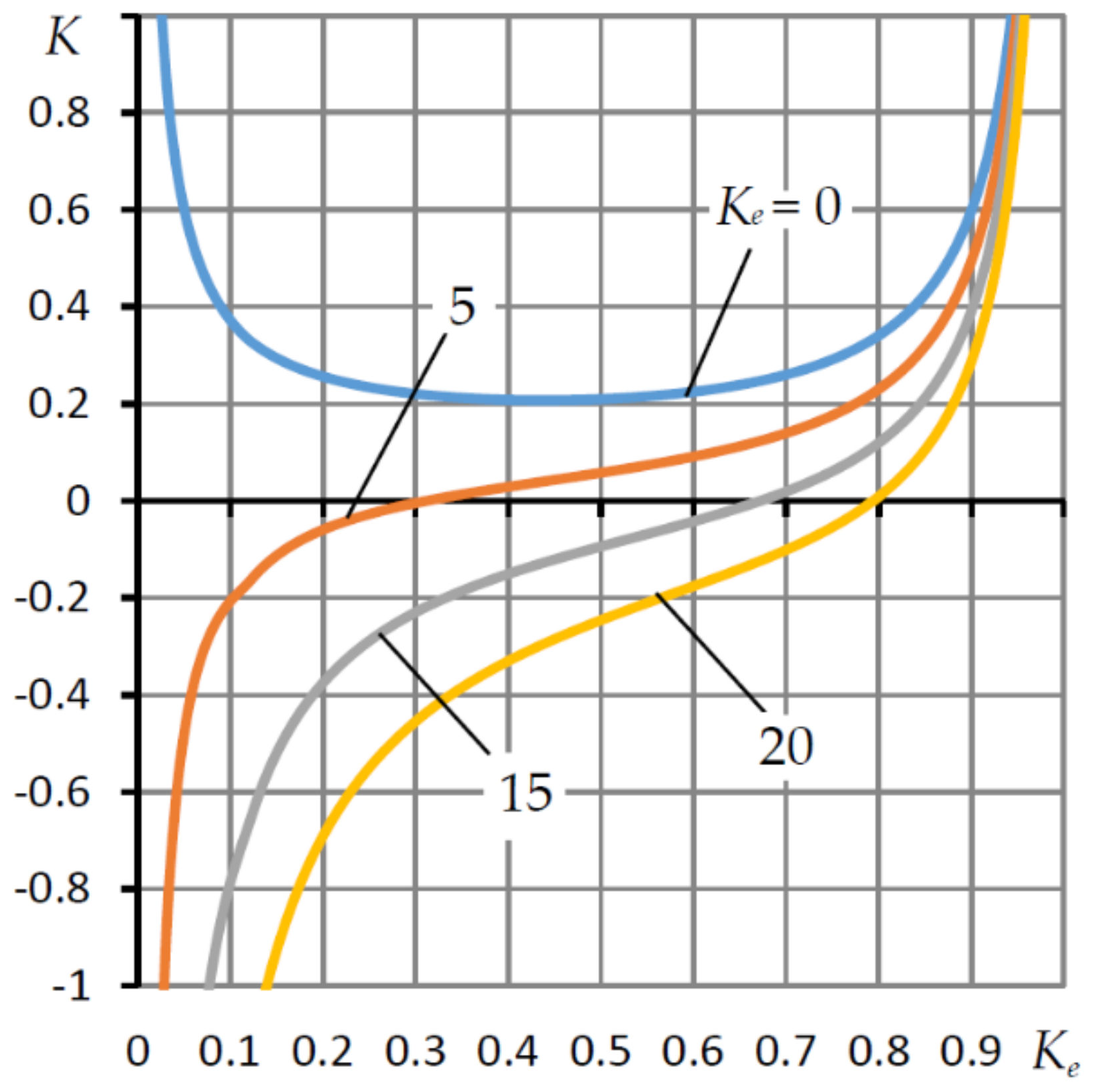
Figure 5 shows the dependences of the compliance K on the adjustment factor χ for different values of the membrane elasticity coefficient K_e for L = 1.5, λ₁ = L₁/L = 0.2, λ₃ = L₃/L = 0.15, P_s = 5 and the recommended value of the weighting factor for the SECT adjustment ς = 0.15 [18,21]. For an absolutely rigid membrane (K_e = 0), the K(K_e) dependence has a unimodal character, with a minimum compliance at χ ≈ 0.45. With an increase in the coefficient of elasticity K_e, the dependences become monotonic. In this case, the smaller χ, the less compliance. It can be seen that the compliance decreases to zero and can reach negative values (K < 0). This phenomenon is explained by the fact that the smaller χ at a small fixed ς, the greater the pressure drop acting on the working surfaces of the annular part, 4, of the sleeve, 3, and, consequently, the higher the activity of the membrane regulator. With an increase in χ, the pressure drop decreases and, along with it, the activity of the regulator decreases, which entails an increase in compliance. Thus, in the presence of membrane elasticity (K_e > 0), a decrease in the adjustment coefficient χ promotes a decrease in compliance. However, if χ is too small, a supersonic air flow through simple diaphragms may occur, which reduces the environmental friendliness of the bearing and contributes to its unstable operation. Therefore, the best values can be considered as χ = 0.4–0.5, at which the characteristic K(K_e) is stable and any compliance can be provided, including negative compliance.

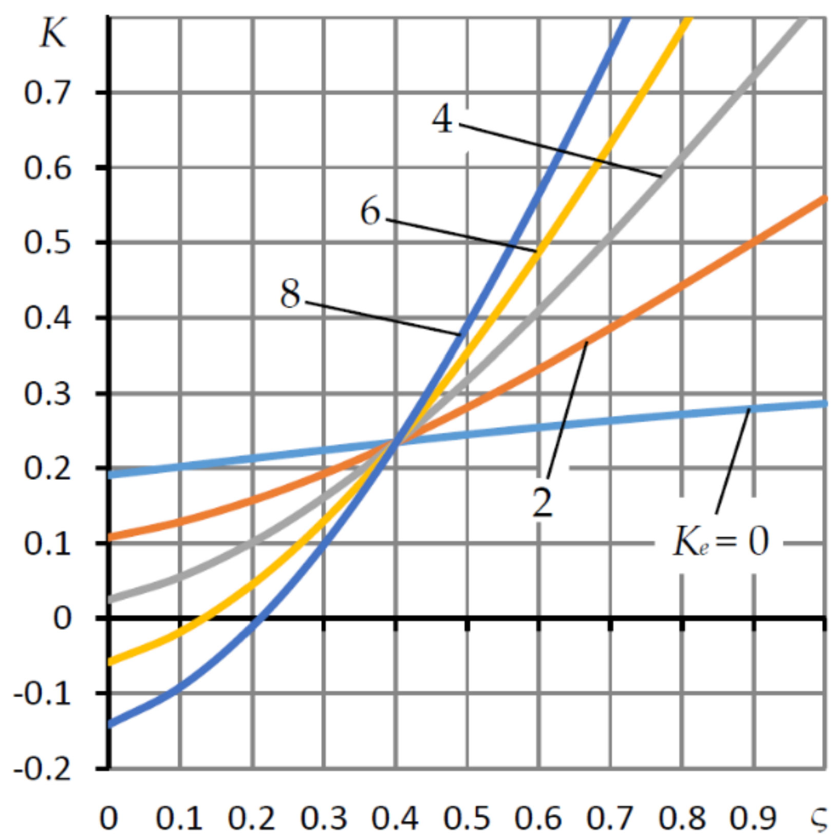
The influence of the weighting factor ς of the SECT resistances is shown in Figure 6. With a rigid suspension and ς = 0, we obtain a single-choke bearing with simple diaphragms, and at ς = 1, a single-choke bearing with annular diaphragms. Such bearings have positive compliance, and in the latter case, as can be seen from the graph, the compliance is 1.5 times higher.

With increasing K_e, the slope of the compliance dependence K(ς) increases. This is explained by the fact that the eccentricity ε receives an additional component ε_p to the eccentricity ε_t, which is formed under the action of the force aerostatic reaction W_p during deformation of the elastic suspension, thereby contributing to a decrease in compliance in the region of small ς and its increase in the region of large ς. In this case, the larger K_e, the steeper the K(ς) curve.

It is seen that for all curves, there is a common point of intersection, which corresponds to ς = ς_c on curves in which the compliance K does not depend on K_e. For those shown in thr Figure 6 data, ς_c ≈ 0.41. From formula (30), it follows that this regime takes place at W_t = W_p, when the aerostatic reactions on the surfaces of the ring, 4, are equal to each other and, therefore, the deformation of the elastic suspension is absent for any K_e. It follows from (41) that ς_c is determined by the solution of the equation

$$A_{wp}{A}_2=A_{wt}{A}_3.$$

It follows from the graphs that a decrease in compliance is possible only under the condition 0 ≤ ς < ς_c. Moreover, the smaller ς, the less the bearing compliance. At the same time, as the study of the dynamics of other types of aerostatic bearings using SECT shows, a decrease in compliance is almost always accompanied by a deterioration in their dynamics up to loss of stability [26,27]. Therefore, to ensure acceptable dynamics, it is recommended to calculate and design low compliance bearings for ς ∈ [0.1, 0.2].

4. Stationary Model of Bearing Operation with Arbitrary Eccentricities

When calculating the load capacity of a bearing with an elastic membrane, it is convenient to vary the eccentricity ${\mathsf{\epsilon }}_t\in \left[0,1\right]$ with a certain small step. To determine the functions P_k(ϕ), P_p(ϕ), it will be necessary to solve the system of nonlinear equations determined by the last two equations (32) of the balance of lubricant flow rate through the resistance of the SECT

$$\left\{\begin{array}{l}{A}_h{H}_t^2\left(P_k^2-1\right)=A_k \mathrm{Brn}\left(P_p,P_k\right),\\ A_h{H}_t^3\left(P_k^2-1\right)=A_p \mathrm{Brn}\left(P_s,P_p\right).\end{array}\right.$$

(42)

We split the segment $\mathsf{\phi }\in [0,\mathsf{\pi }]$ into an even number m of parts and, for a given ε_t, we will solve the system of equations (42) for ${\mathsf{\phi }}_j=\frac{\mathsf{\pi }j}{m},j=0,1,\dots ,m.$ Let us simplify the problem by reducing the system of equations to a single equation with respect to the unknown pressure P_p(ϕ_j). To do this, we express from the last equation $P_k=\sqrt{1+\frac{A_p \mathrm{Brn}\left(P_s,P_p\right)}{A_h{H}_t^3}}$ and substitute it into the first Equation (42). In this case, only one unknown pressure P_p(ϕ_j) will remain. The problem was solved by bracketing using the bisection method on a segment. In the process of solving, the corresponding pressure P_k(ϕ_j) is simultaneously calculated.

After determining the pressures P_k,j = P_k(ϕ_j), P_p,j = P_p(ϕ_j), (j = 0,1,…, m), the reactions W_c, W_t and W_p were found by numerical integration using the Simpson formula [30]

$$W_t=\frac{4L_1}{9m}{\displaystyle \sum _{j=0}^m{g}_j\frac{P_{k,j}^3-1}{P_{k,j}^2-1}},W_c=\frac{2L_2}{3m}{\displaystyle \sum _{j=0}^m{g}_j{P}_{k,j}},W_p=\frac{2R_1{L}_3}{3m}{\displaystyle \sum _{j=0}^m{g}_j{P}_{p,j}},$$

where $g_j=s_j{c}_j,$ $c_j=\cos \left(\frac{\mathsf{\pi }j}{m}\right),$ s_j are the coefficients of the Simpson formula [30].

Further, the load-bearing capacity W = W_t + W_c, the deformation ε_p of the membrane according to the second formula (32) and the eccentricity ε according to the third formula (32) were determined. Calculations have shown that an accuracy sufficient for practice is achieved by dividing the integration interval into m = 32 parts. When solving system (42), the pressures were determined with an accuracy of 10⁻¹². Such accuracy was required to find the load capacity for extremely large values of the eccentricity ε_p.

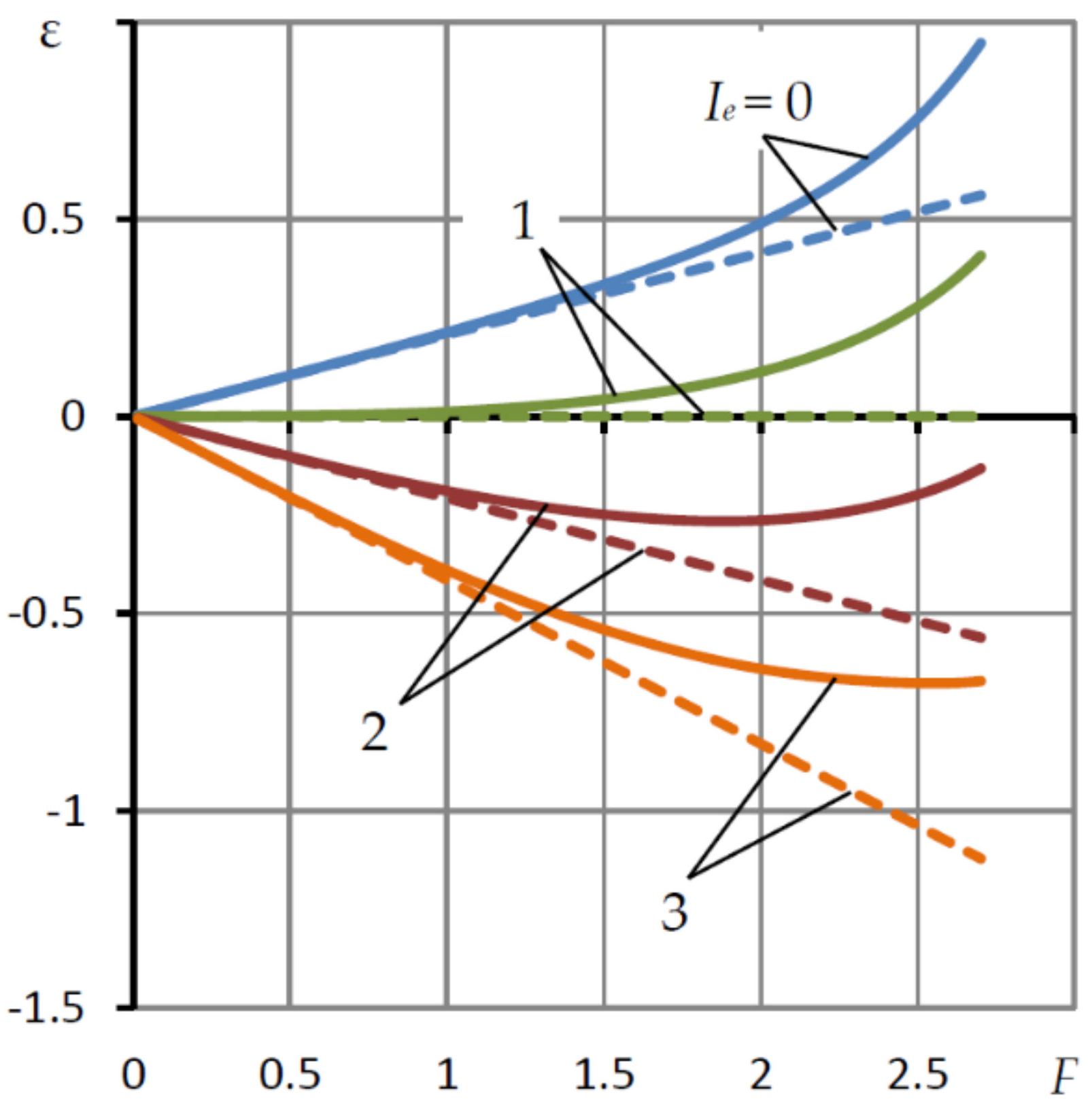
In Figure 7, solid lines show the dependences of the eccentricity ε on the external load F = W at various values of the elasticity coefficient K_e = I_e K_e0, where K_e0 is calculated by formula (41). Dashed lines represent linear dependences of the form $\mathsf{\epsilon }=K\times W,$ where K is the static compliance of the bearing, calculated by the Formula (40). The parameters remain fixed with the values that were used when plotting the graph in Figure 5. Lines I_e = 0 correspond to a bearing with a rigid membrane, that is, a conventional two-row bearing with longitudinal microgrooves [29]. With I_e = 1, we obtain a bearing with zero compliance (K_e = K_e0, K = 0) in the vicinity of the central equilibrium arrangement of the moving elements. Lines I_e > 1 correspond to a bearing with negative compliance in this vicinity. The maximum load capacity of the bearing with the specified parameters corresponds to W_max ≈ 2.8.

It can be seen that the solid and dashed dependences practically do not differ at 0 ≤ F ≤ 0.5 and differ slightly from each other at 0.5 ≤ F ≤ 1. This means that the load characteristics of the bearing with longitudinal microgrooves and a membrane regulator remain practically linear in the range up to 35% of permissible bearing loads. This circumstance is important for bearings of negative compliance, which are designed to be used both as supporting elements of metal-cutting machines and as automatic compensators for small deformations of their technological system, which, due to their smallness, obey Hooke’s law and, therefore, are linearly related to the cutting force. The addition of two linear functions opposite in sign will make it possible to almost completely eliminate the negative influence of the deformation of the machine tool technological system on the processing quality.

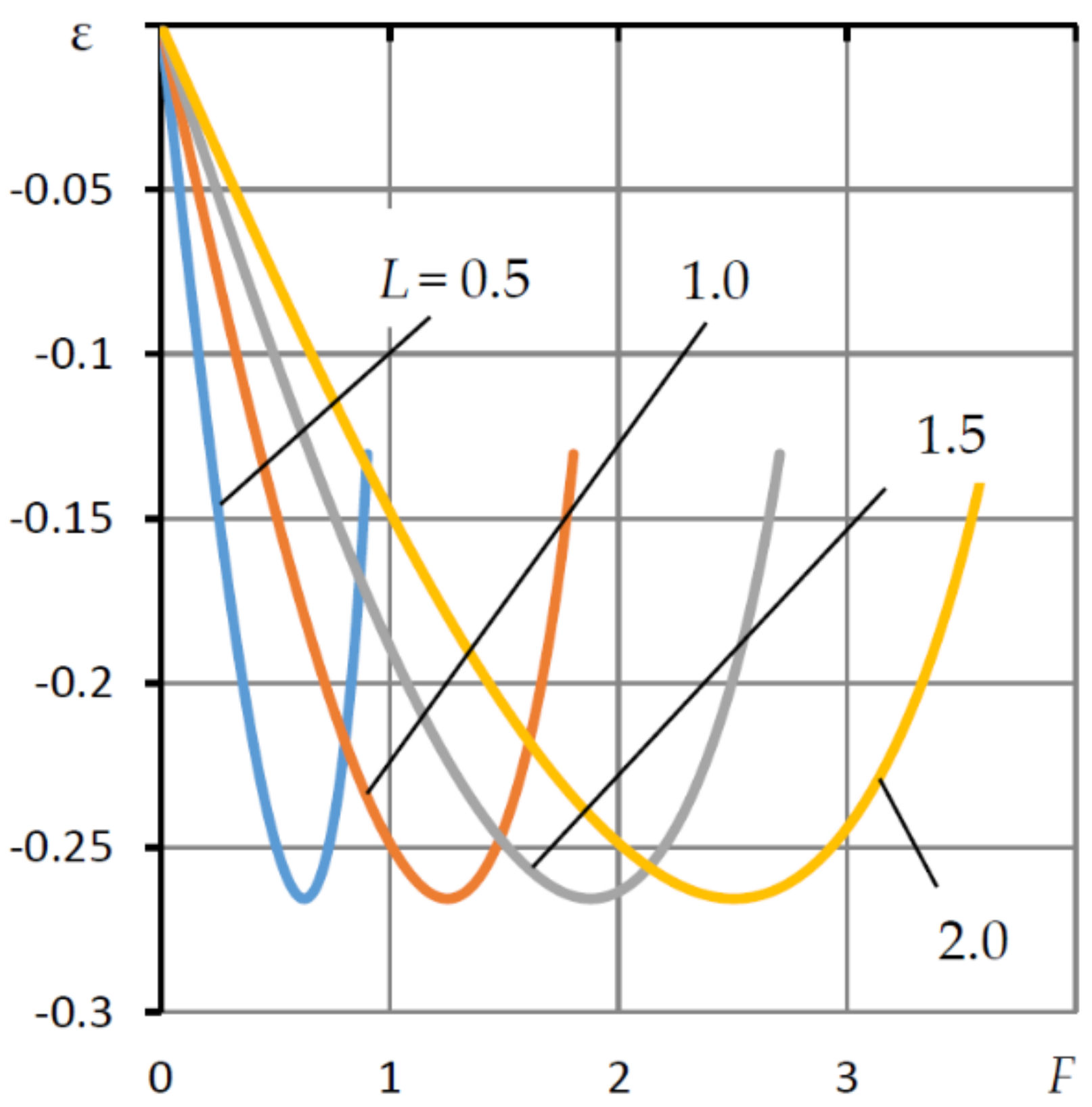
Figure 8 shows the load curves ε(F) for different values L of the bearing length at K_e = 2K_e0.

A bearing with such parameters in the area of low and moderate loads has a negative compliance (K < 0). Analysis of the data showed that the negative compliance mode remains in the range up to 66% of the maximum allowable bearing load. These dependences characterize the main advantage of aerostatic radial bearings with longitudinal microgrooves, which, in contrast to conventional bearings with smooth running surfaces, have the ability to provide significantly higher load-bearing capacity due to the almost complete elimination of circumferential leakage of compressed air in the inter-row zone [29]. For L > 1, the presence of this improvement provides an increase in the load capacity of the bearing by a factor of 1.5 or more.

The expansion of the load range is also facilitated by a decrease in the adjustment factor χ of the SECT. However, in comparison with the effect of the presence of microgrooves, this effect is insignificant. The final decision on the optimality of the parameters that affect the static compliance and load capacity can be given only by comparing these characteristics with the dynamic quality criteria, which allow us to establish the modes of the fastest response and guaranteed stability margin in order to minimize the oscillation of the transient characteristics in the operating range of loads.

5. Non-Stationary Model of the Bearing at Small Deviations from the Central Equilibrium Position of the Moving Elements

It is known that loading is a factor that has a positive effect on the dynamic characteristics of aerostatic bearings [31]. Therefore, to assess the quality of the dynamics of a structure, it is sufficient to study its dynamic properties at small oscillations in the vicinity of the central position of the moving elements.

The pressure function P(Z,φ,τ) in the bearing gap in the absence of circumferential lubricant flows satisfies the dimensionless unsteady Reynolds equation [32]

$$\frac{\partial }{\partial Z}\left(H_i^{3}P\frac{\partial P}{\partial Z}\right)=\mathsf{\sigma }\frac{\partial \left(P{H}_i\right)}{\partial \mathsf{\tau }},$$

(43)

where τ is dimensionless time; $\mathsf{\sigma }=\frac{12\mathsf{\mu }{r}_0^2}{h_0^2{p}_a{t}_0}$ is the so-called compression number [31], t₀ is the current time scale and H_i is any of the gaps

$$H_t(\mathsf{\phi },\mathsf{\tau })=1-\Delta {\mathsf{\epsilon }}_t(\mathsf{\tau })\cos \mathsf{\phi },$$

(44)

$$H(\mathsf{\phi },\mathsf{\tau })=1-\Delta \mathsf{\epsilon }(\mathsf{\tau })\cos \mathsf{\phi }$$

(45)

at low loads ΔF(τ).

On pressurization lines

$$P_k(\mathsf{\phi },\mathsf{\tau })=P_{k0}+\Delta P_k(\mathsf{\tau })\cos \mathsf{\phi },$$

(46)

$$P_p(\mathsf{\phi },\mathsf{\tau })=P_{p0}+\Delta P_p(\mathsf{\tau })\cos \mathsf{\phi }.$$

(47)

By analogy with this, we represent the pressure distributed in the lubricant gap in the form

$$P(Z,\mathsf{\phi },\mathsf{\tau })=P_0(Z)+\Delta P(Z,\mathsf{\tau })\cos \mathsf{\phi }.$$

(48)

Substituting (44)–(48) into (43), performing linearization and the subsequent Laplace transform [33], we obtained the problem for the required transform $\overline{\Delta P}$ in the inter-row and outer zones

$$\left\{\begin{array}{l}\frac{d^2\left(P_0\overline{\Delta P}\right)}{d{Z}^2}-\mathsf{\sigma }s\left(\overline{\Delta P}-P_0{\overline{\Delta \mathsf{\epsilon }}}_i\right)=0,\\ \frac{d\overline{\Delta P}}{dZ}(0,s)=0,\hspace{0.33em}\overline{\Delta P}(L_2,s)={\overline{\Delta P}}_k,\overline{\Delta P}(L,s)=0.\end{array}\right.$$

(49)

Here, s is the variable of the Laplace transform, ${\overline{\Delta P}}_k(s),\overline{\Delta P}(s)\overline{,\Delta {\mathsf{\epsilon }}_i}(s)$ are the Laplace transformants of the deviations of the pressures P, Pk and of the eccentricities from their equilibrium state and position.

For the outer zone, problem (49) has no analytical solution; therefore, we solve it by the numerical finite-difference sweep method [34]. For this, we represent its solution in the form of a linear combination

$$\overline{\Delta P}=U_p(Z,s){\overline{\Delta P}}_k+U_{\mathsf{\epsilon }}(Z,s){\overline{\Delta \mathsf{\epsilon }}}_t.$$

(50)

Substituting (50) into (49) and performing the separation of transformants, we obtain two boundary value problems for the functions U, which can be represented in the following general form

$$\left\{\begin{array}{l}\frac{d^2}{d{Z}^2}\left(P_{0}U\right)-\mathsf{\sigma }sU+\mathsf{\alpha }{P}_0=0,\\ U(0)=(1-\mathsf{\alpha }),U(L_1)=0,\end{array}\right.$$

(51)

where α = 0 corresponds to U_p, α = 1 corresponds to U_e.

To find a solution to problem (51), we divide the interval of integration [0, L₁] into an even number n of equal parts and replace the differential equations with their algebraic analogs

$$\frac{P_0^{i+1}{U}_{i+1}-2P_0^i{U}_i+P_0^{i-1}{U}_{i-1}}{{\mathsf{\nu }}^2}-\mathsf{\sigma }s{U}_i+\mathsf{\alpha }{P}_0^i=0,$$

(52)

where ν = L₁/n is the grid step, i = 1, 2, …, n–1 is the number of its node and $P_0^i=P_0(Z_i),Z_i=i\mathsf{\nu }.$

The solution to problem (51) was found by the sweep method in the form

$$U_{i-1}=X_i{U}_i+Y_i,$$

(53)

where X_j, Y_j are sweep coefficients.

Substituting (53) into (52), we found recurrent formulas for the sweep coefficients

$$X_{i+1}=\frac{P_0^{i+1}}{2P_0^i-P_0^{i-1}{X}_i+{\mathsf{\sigma }\mathsf{\nu }}^{2}s},Y_{i+1}=\frac{P_0^{i-1}{Y}_i+{\mathsf{\sigma }\mathsf{\nu }}^2{P}_0^{i}s}{2P_0^i-P_0^{i-1}{X}_i+{\mathsf{\sigma }\mathsf{\nu }}^{2}s}.$$

(54)

Comparing (54) with (53) for i = 1, we found the initial sweep coefficients for the direct sweep

$$X_1=0,Y_1=1-\mathsf{\alpha }.$$

Performing a sweep for α = 0 and α = 1 using the Simpson numerical quadrature formula, we determined the coefficients

$$A_{wtp}=\frac{\mathsf{\nu }}{3}{\displaystyle \sum _{i=0}^n{c}_i}{U}_{p,i},A_{wte}=\frac{\mathsf{\nu }}{3}{\displaystyle \sum _{i=0}^n{c}_i}{U}_{e,i},$$

where c_i are the coefficients of the Simpson quadrature formula [30].

Load-bearing capacity transformants in the outer zone are

$${\overline{\Delta W}}_t=A_{wtp}{\overline{\Delta P}}_k+A_{wte}{\overline{\Delta \mathsf{\epsilon }}}_t.$$

(55)

The transformant of the flow rate in the bearing gap on the pressurization line in the outer zone at Z = 0 is determined by the expression

$${\overline{\Delta Q}}_{ht}=-2\frac{d\left(P_0\overline{\Delta P}\right)}{dZ}+3\frac{d{P}_0^2}{dZ}{\overline{\Delta \mathsf{\epsilon }}}_t.$$

(56)

Substituting the numerical formula of the first derivative of the second order accuracy [34] at the point Z = 0, we found

$${\overline{\Delta Q}}_{ht}=C_{qtp}{\overline{\Delta \mathrm{P}}}_k+C_{qte}{\overline{\Delta \mathsf{\epsilon }}}_t,$$

(57)

where $C_{qtp}=\frac{P_0^2{U}_{p,2}-4P_0^1{U}_{p,2}+3P_0^0{U}_{p,2}}{\mathsf{\nu }},C_{qte}=-3Q_{h0}.$

For the inter-row zone, problem (49) admits an analytical solution

$$\overline{\Delta P}=\frac{\mathrm{ch}\left(\mathsf{\lambda }Z\right)}{\mathrm{ch}\left(\mathsf{\lambda }{L}_2\right)}{\overline{\Delta P}}_k+P_{k0}\left[1-\frac{\mathrm{ch}\left(\mathsf{\lambda }Z\right)}{\mathrm{ch}\left(\mathsf{\lambda }{L}_2\right)}\right]\overline{\Delta \mathsf{\epsilon }},$$

(58)

where ${\mathsf{\lambda }}^2=\frac{\mathsf{\sigma }s}{P_{k0}}.$

After integrating (58), we found

$${\overline{\Delta W}}_c=C_{wcp}{\overline{\Delta P}}_k+C_{wce}\overline{\Delta \mathsf{\epsilon }},$$

(59)

where $C_{wcp}=\frac{\mathrm{th}\left(\mathsf{\lambda }{L}_2\right)}{\mathsf{\lambda }},C_{wce}=P_{k0}\left(L_2-C_{wcp}\right).$

The transformant of the flow rate in the bearing gap on the pressurization line in the inter-row zone at Z = L₂ is equal to

$${\overline{\Delta Q}}_{hc}=2P_{k0}\frac{d\overline{\Delta P}}{dZ}=C_{qcp}{\overline{\Delta P}}_k{C}_{qce}\overline{\Delta \mathsf{\epsilon }},$$

(60)

where $C_{qcp}=2\mathsf{\lambda }{P}_{k0}\mathrm{th}\left(\mathsf{\lambda }{L}_2\right),c_{qce}=-P_{k0}{C}_{qcp}.$

Expressions for the transformants of the flow rate through annular diaphragms and through simple diaphragms are, respectively

$${\overline{\Delta Q}}_k=A_{qkk}{\overline{\Delta P}}_k+A_{qkp}{\overline{\Delta P}}_p-A_{qke}{\overline{\Delta \mathsf{\epsilon }}}_t,$$

(61)

$${\overline{\Delta Q}}_p=A_{qpp}{\overline{\Delta P}}_p.$$

(62)

The compressibility of the lubricant in the inter-throttle chambers of the dimensionless volume V_p and the microgrooves of the dimensionless volume V_k was taken into account using the flow rate transformants

$${\overline{\Delta Q}}_{vp}=A_{vp}{\overline{\Delta P}}_p,$$

(63)

$${\overline{\Delta Q}}_{vk}=A_{vk}{\overline{\Delta P}}_k,$$

(64)

where $A_{vp}=2\mathsf{\sigma }L{V}_p,A_{vk}=2\mathsf{\sigma }L{V}_k.$

Finally, the force of inertia of the shaft mass was taken into account using the formula

$${\overline{\Delta F}}_i=Mas\times s^2\overline{\Delta \mathsf{\epsilon }},$$

(65)

where Mas is the dimensionless shaft mass.

The system of equations describing the balance of forces, displacements, and mass flow rates has the form

$$\left\{\begin{array}{l}{\overline{\Delta W}}_t+{\overline{\Delta W}}_c+{\overline{\Delta F}}_i=\overline{\Delta F},\\ {\overline{\Delta \mathsf{\epsilon }}}_t+K_e\left({\overline{\Delta W}}_p-{\overline{\Delta W}}_t\right)=0,\\ \overline{\Delta \mathsf{\epsilon }}-{\overline{\Delta \mathsf{\epsilon }}}_t-{\overline{\Delta \mathsf{\epsilon }}}_p=0,\\ {\overline{\Delta Q}}_p-{\overline{\Delta Q}}_{vp}-{\overline{\Delta Q}}_k=0,\\ {\overline{\Delta Q}}_k-{\overline{\Delta Q}}_{vk}-{\overline{\Delta Q}}_{ht}-{\overline{\Delta Q}}_{hc}=0.\end{array}\right.$$

(66)

Substituting (55)–(65) in (66), we obtained a system of linear equations with a Laplace image of the disturbing input external force $\overline{\Delta F}(s)$ and images of the output functions $\overline{\Delta \mathsf{\epsilon }}(s),{\overline{\Delta \mathsf{\epsilon }}}_t(s),{\overline{\Delta \mathsf{\epsilon }}}_p(s),{\overline{\Delta P}}_k(s),{\overline{\Delta P}}_p(s).$ Dividing equations (66) by $\overline{\Delta F}$, we obtained the corresponding system of equations for dynamic transfer functions

$$K(s)=\frac{\overline{\Delta \mathsf{\epsilon }}}{\overline{\Delta F}},K_{et}(s)=\frac{{\overline{\Delta \mathsf{\epsilon }}}_t}{\overline{\Delta F}},K_{ep}(s)=\frac{{\overline{\Delta \mathsf{\epsilon }}}_p}{\overline{\Delta F}},K_{pk}(s)=\frac{{\overline{\Delta P}}_k}{\overline{\Delta F}},K_{pp}(s)=\frac{{\overline{\Delta P}}_p}{\overline{\Delta F}}.$$

The first of them is the transfer function of interest to us, K(s), of the dynamic compliance of the bearing, and K(0) is its static compliance.

System (66) has the following matrix form

$$\left[\begin{array}{ccccc}{B}_{11}& B_{12}& B_{13}& B_{14}& 0\\ 0& B_{22}& B_{23}& B_{24}& B_{25}\\ 1& -1& -1& 0& 0\\ B_{41}& B_{42}& 0& B_{44}& B_{45}\\ 0& B_{52}& 0& B_{54}& B_{55}\end{array}\right]\left[\begin{array}{c}K\\ K_{et}\\ K_{ep}\\ K_{pk}\\ K_{pp}\end{array}\right]=\left[\begin{array}{c}1\\ 0\\ 0\\ 0\\ 0\end{array}\right],$$

(67)

where

$$\begin{array}{l}{B}_{11}=A_{wce}+Mas\times s^2,B_{12}=A_{wte},B_{14}=A_{wtp}+A_{wcp},\\ B_{22}=-K_e{A}_{wte},B_{24}=-K_e{A}_{wtp},B_{25}=K_e{A}_{wpp},\\ B_{41}=-A_{qce},B_{42}=-\left(A_{qke}+A_{qte}\right),\\ B_{44}=A_{qkk}-A_{qtp}-A_{qcp}-A_{vk},B_{45}=A_{qkp},\\ B_{52}=A_{qke},B_{54}=-A_{qkk},B_{55}=A_{qpp}-A_{qkp}-A_{vp}.\end{array}$$

(68)

6. Bearing Dynamic Characteristics

The mathematical model of the dynamics of small oscillations, represented by the system of Equation (67), is a system with distributed parameters since it was obtained by numerically solving a boundary value problem for a differential equation. The transfer function (TF) of the compliance of such a system is generally a transcendental function. We will approximately represent it by an equivalent rational function in the form of the ratio of the polynomials of the Laplace variable s. The rational interpolation method is described in detail in [27,35]. In accordance with it, the TF was represented in the form

$$K(s)=\frac{\overline{\Delta H}}{\overline{\Delta F}}=\frac{b_0+b_{1}s+b_2{s}^2+\dots +b_m{s}^m}{1+a_{1}s+a_2{s}^2+\dots +a_n{s}^n},$$

(69)

where n > 0, m > 0, n > m.

The denominator of the ratio (30) is a characteristic polynomial (CP), the use of which in the study of the quality of the bearing dynamics allows us to determine the stability margin and assess the speed of the system by the roots of the CP [33].

The difference in the orders of the polynomials d was determined for a_n ≠ 0 and b_m ≠ 0 by finding the infinite limit

$$s^{d}K(s)\to \frac{b_m}{a_n}\ne 0.$$

(70)

It was found that d = 2.

To assess the quality of the dynamics of linear systems, root criteria are often used [33]:

–

the degree of stability $\mathsf{\eta }=\mathrm{Max}\hspace{0.33em}\mathrm{Re}\left\{s_i\right\}$, where s_i are the zeros of the characteristic polynomial of the dynamical system, which is the denominator polynomial of the TF (69)

–

damping of oscillations for a period $\mathsf{\xi }=100[1-\mathrm{Exp}(-\left|2\mathsf{\pi }\mathsf{\beta }/\mathsf{\eta }\right|]\%,$ where β is the imaginary part of the root of the characteristic equation with the largest real part.

The degree of stability η characterizes the speed of the system, that is, the speed of damping of its free oscillations.

The criterion ξ of oscillations damping over a period can be applied to the assessment of the system’s stability margin. The smaller ξ, the more oscillation the transient response will have, and the system will have a smaller stability margin. It is believed that a dynamic system is well damped if ξ ≥ 90% [33].

When determining the criteria for dynamic quality, an iterative algorithm was used, the essence of which is to find the smallest degree of CP n, at which, after finding the criteria, the conditions for the convergence of the iterative process are satisfied

$$\left|{\mathsf{\eta }}_i-{\mathsf{\eta }}_{i-1}\right|<{\mathsf{\epsilon }}_{\mathsf{\eta }},\hspace{1em}\hspace{1em}\left|{\mathsf{\xi }}_i-{\mathsf{\xi }}_{i-1}\right|<{\mathsf{\epsilon }}_{\mathsf{\xi }},$$

(71)

where i is the iteration number and ${\mathsf{\epsilon }}_{\mathsf{\eta }},{\mathsf{\epsilon }}_{\mathsf{\xi }}$ is the accuracy of determining the criteria. Calculations have shown that the accuracy ${\mathsf{\epsilon }}_{\mathsf{\eta }}={10}^{-4},{\mathsf{\epsilon }}_{\mathsf{\xi }}=0.1$ is achieved at the degree of CP n = 4 ÷ 10, depending on the set of values of the input parameters.

Figure 9, Figure 10, Figure 11 and Figure 12 show the dependences for the criteria η, ξ of the bearing dynamic quality for the following fixed values of the parameters: L = 1.5, λ₁ = L₁/L = 0.2, λ₃ = L₃/L = 0.15, R₁ = 1.1, χ = 0.45, ς = 0.15, P_s = 5, Mas = 1 and the dimensionless volume of microgrooves V_k = 0.03. The latter value is based on the results of studying the static characteristics of a conventional aerostatic radial bearing with longitudinal microgrooves in the inter-row zone [29]. This value gives an estimate of the volume of microgrooves at which there are practically no circumferential leakages of compressed air. On this basis, when studying both static and dynamic characteristics, in spatial coordinates, only the axial flow of the lubricant can be taken into account. It is on this position that mathematical models of the statics and dynamics of the bearing under study are based.

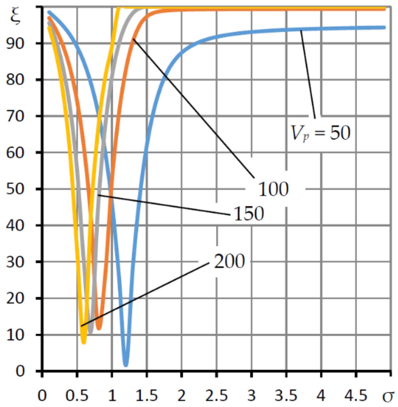
Figure 9 shows the dependence of the degree of stability η on the compression number σ, for various values of the dimensionless volume of the inter-throttling cavities V_p, which only affect the dynamic quality of the bearing. The presented graphs confirm the main property of aerostatic bearings with SECT, which consists in the fact that in the space of these parameters the criterion of speed η has a single extremum, which is the boundary between the oscillatory and aperiodic transient characteristics of the output functions arising from an external force action.

The graphs in Figure 9 are plotted for the membrane elasticity coefficient K_e = 2K_e0, at which the bearing has negative static compliance (K < 0), which is the same in absolute value as the compliance of a conventional bearing with a rigid membrane. It is seen that for small σ the bearing is always unstable. Since the value of σ is inversely proportional to the square of the thickness of the bearing gap h₀², this means that for a stable bearing there is a limitation on the size of the gap, which is determined by the stability boundary (η = 0). It can be seen from the graphs that this boundary also depends on the value of the volume V_p. For small volumes, the stability boundary is shifted to the right, that is, for small volumes V_p, stability is ensured with smaller gaps. With an increase in V_p, the boundary shifts to the left, therefore, when designing a stable bearing, if necessary, the gap can be increased.

Noteworthy is the η (σ) curve corresponding to V_p = 200, which has two extrema. As the analysis of dependencies corresponding to large values of the volume V_p has shown, the dominant effect on the bearing speed is exerted not by one, which is typical for small and moderate V_p, but by two roots of the characteristic equation. Their interaction gives the noted effect.

It can also be seen that the curves η (σ) have an extreme character, reaching their maximum at the point σ = σ_opt, which delivers the bearing the maximum response speed as a dynamic system, providing the fastest damping of transient processes caused by external force on the shaft, 2. On the graph in Figure 9, this corresponds to σ_opt ≈ 1.5. If we compare the curves in Figure 9 and Figure 10, the last of which shows the dependence of the damping criterion on σ for the period ξ, it can be concluded that at σ < σ_opt, the transient characteristics are oscillatory (ξ < 100%), which indicates an insufficient bearing stability margin. However, at σ > σ_opt, and sufficiently large volumes V_p, the transient characteristics acquire aperiodic character (ξ = 100%). This indicates a high margin of stability. Thus, the parameters σ and V_p are important factors for ensuring not only stability, but also the quality of the transient characteristics of the bearing of low compliance, including negative ones. Noteworthy is the fact that the dependences η(V_p) are also extreme. This follows from the fact that, with increasing V_p, the peaks of the η (σ) dependences first increase and then decrease. This means that there is an optimal volume V_p = V_p,opt. The analysis of the graphs showed that with an increase in V_p, the oscillation of the transient characteristics decreases (ξ increases). At V_p = V_p,opt, the transient characteristics become aperiodic (ξ = 100%). At V_p > V_p,opt, the aperiodic character of the characteristics does not change, however, the bearing speed begins to decrease, which is expressed in a decrease in the value of the criterion η. At the same time, the calculation of bearing parameters based on the maximum performance indicators η, which takes place at σ = σ_opt, V_p = V_p,opt, is not the best. It is preferable to give up some speed, however, to provide a guaranteed stability margin (ξ = 100%), choosing σ> σ_opt, V_p > V_p,opt near the extremum η. For the graphs in Figure 9 and Figure 10, such values can be σ = 2–2.5, V_p = 200.

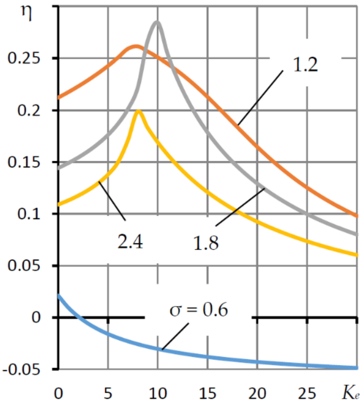
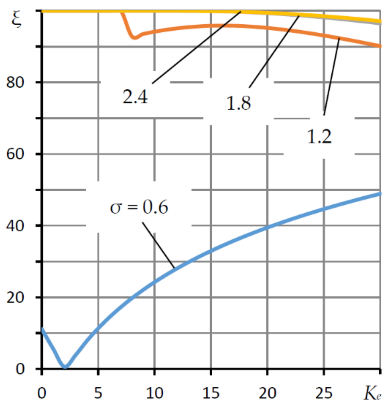
Figure 11 and Figure 12 show the dependences of the criteria η, ξ on the coefficient of elasticity K_e for different values of σ. For small σ = 0.6, the bearing is stable only for small K_e, which corresponds to a conventional bearing. At higher σ, the η(K_e) dependences acquire an extreme character, reaching a maximum. Comparison of these curves with the dependences of static compliance K(K_e) (Figure 2) shows that the maximum response rate falls on the zero-compliance mode. A further increase in K_e leads to a decrease in the bearing speed, but it remains stable (η > 0).

As can be seen from the graph in Figure 12, a bearing with zero and negative compliance has a large stability margin (ξ = 100%). Only if the membrane compliance is too high, the stability margin decreases slightly (ξ = 97%). Nevertheless, it remains sufficient to consider the bearing as a well-damped dynamic system.

When studying the dynamics of a bearing with a lubricant output flow’s limitation, the effect of the volume of microgrooves on the dynamic characteristics of the structure was studied. It was found that within the limits of the volumes of the microgrooves, which ensure the neutralization of the negative influence of circumferential flows (V_k ≤ 0.03), they do not have a noticeable effect on the bearing dynamics.

7. Conclusions

The paper considers a two-row symmetric aerostatic radial bearing with an external combined throttling throttle system, longitudinal microgrooves in the inter-row area and an air lubricant outlet flow rate regulator. The aim of the work is to substantiate the assumption that the use of output limiters can significantly reduce the bearing compliance down to zero and negative values. Since the use of flow controllers usually entails a deterioration in the dynamics of aerostatic bearings up to the loss of stability, a well-proven system of external combined throttling is used in the design, where simple diaphragms are used as the main resistance, and annular diaphragms are used as additional damping resistances. An important factor in ensuring stability and improving the quality of dynamics are the volumes of flow-through inter-throttle chambers.

To carry out the research, mathematical modeling, calculation and theoretical study of stationary operating modes of the bearing were carried out. The study of compliance for small eccentricities of moving elements in the vicinity of the central equilibrium position of the shaft, as well as the load capacity for arbitrary eccentricities was carried out. Formulas for determining static compliance and load-bearing capacity are obtained. Iterative finite-difference methods for determining the dynamic characteristics of a structure are proposed. The calculation of dynamic quality criteria was carried out on the basis of the method of rational interpolation of the bearing transfer function, as a system with distributed parameters, developed by the authors.

It was found that the volumes of the microgrooves do not have a noticeable effect on the bearing dynamics. It is shown that, in this design, the external throttling system is an effective means of maintaining the stability of the structure operating in the modes of low, zero and negative compliance.

Thus, the considered two-row aerostatic radial bearing with a system of external combined throttling, longitudinal microgrooves in the inter-row area and a regulator of the flow rate of the lubricant output flow can find practical application as a supporting structure of metal-cutting machines in the presence of negative compliance. At the same time it can be applied as an automatic compensator of elastic deformation of technological systems in order to reduce time and improve the accuracy of metalworking.

When designing a bearing, in order to obtain the minimum compliance and ensure optimal dynamic criteria, it is recommended to select the values of the adjustment factors 0.4 < χ < 0.5 and 0.1 < ς < 0.2. Such a choice allows to provide any low as well as negative compliance. To eliminate the negative effect of circumferential air leakage, at least 12 microgrooves must be made in the inter-row zone. In this case, the total volume of microgrooves should be two orders of magnitude less than the volume of the bearing air layer. The depth and width of the microgrooves should be 3–5 times greater than the air gap h₀ with the central location of the movable elements. The bearing has the maximum degree of stability at the optimal values of the compression number σ and the dimensionless volume of the inter-throttle chambers V_p, which follows from the presented graphs. The choice of close to the optimal value of σ allows calculating the size of the central gap h₀, at which the bearing will have the optimal values of the criterion of speed and stability η and the stability margin ξ. From the value of the dimensionless volume V_p, at which the best dynamics of the structure is ensured, it is possible to calculate the optimal dimensional volume of the inter-throttle chambers.