New Approaches to the General Linearization Problem of Jacobi Polynomials Based on Moments and Connection Formulas

Abstract

This article deals with the general linearization problem of Jacobi polynomials. We provide two approaches for finding closed analytical forms of the linearization coefficients of these polynomials. The first approach is built on establishing a new formula in which the moments of the shifted Jacobi polynomials are expressed in terms of other shifted Jacobi polynomials. The derived moments formula involves a hypergeometric function of the type $4F_3\left(1\right)$, which cannot be summed in general, but for special choices of the involved parameters, it can be summed. The reduced moments formulas lead to establishing new linearization formulas of certain parameters of Jacobi polynomials. Another approach for obtaining other linearization formulas of some Jacobi polynomials depends on making use of the connection formulas between two different Jacobi polynomials. In the two suggested approaches, we utilize some standard reduction formulas for certain hypergeometric functions of the unit argument such as Watson’s and Chu-Vandermonde identities. Furthermore, some symbolic algebraic computations such as the algorithms of Zeilberger, Petkovsek and van Hoeij may be utilized for the same purpose. As an application of some of the derived linearization formulas, we propose a numerical algorithm to solve the non-linear Riccati differential equation based on the application of the spectral tau method.

1. Introduction

Special functions are crucial in several disciplines such as mathematical physics and numerical analysis. A large number of researchers are interested in investigating different special functions from numerical and practical points of view; see, for example, [1,2,3].

Jacobi polynomials are of basic importance in mathematical analysis from both theoretical and practical points of view. There are six important particular classes of Jacobi polynomials. In fact, ultraspherical, Legendre, and Chebyshev polynomials of the first- and second- kinds are symmetric Jacobi polynomials, while the two classes of Chebyshev polynomials of third- and fourth- kinds are non-symmetric Jacobi polynomials (see, for example, [4,5,6]). The linearization and connection problems of different orthogonal polynomials are of fundamental importance. They play a role in the computation of physical and chemical properties of quantum-mechanical systems [7]. The standard linearization formula is applied in the calculation of the position and momentum information entropies of quantum systems (see Dehesa et al. [8]). Furthermore, they are useful in treating some kinds of differential equations. For example, Abd-Elhameed [9] has employed some linearization formulas to solve a non-linear Riccati differential equation. Recently, Abd-Elhameed in [10] employed the linearization formula of the shifted Chebyshev polynomials of the sixth-kind along with some other formulas to develop a spectral solution to the one-dimensional non-linear Burgers’ equation. Due to the importance of the linearization formulas, intensive studies regarding these problems have been performed. Linearization and connection problems for a variety of classical continuous and discrete orthogonal polynomials have been established by many methods (see, for instance, [11,12,13,14,15,16,17,18,19,20]).

If we assume three families of polynomials ${\left\{{\varphi }_i\left(x\right)\right\}}_{i\ge 0}$ ${\left\{{\psi }_j\left(x\right)\right\}}_{j\ge 0}$ and ${\left\{{\theta }_k\left(x\right)\right\}}_{k\ge 0}$, then to solve the general linearization problem

$${\displaystyle {\varphi }_i\left(x\right){\psi }_j\left(x\right)=\sum _{k=0}^{i+j}{A}_{k,i,j}{\theta }_k\left(x\right),}$$

we have to find the linearization coefficients $A_{k,i,j}$.

It is worth mentioning here that among the important problems that are related to the linearization problems are the problems concerned with summing the finite products of several special functions. In this direction, the authors of [21], developed some results for the sums of finite products of the second, third, and fourth kinds Chebyshev polynomials. In [22], the authors studied the connection problem for sums of finite products of Chebyshev polynomials of the third and fourth kinds. Expressions for sums of finite products of Legendre and Laguerre polynomials can be found in [23]. In [24], the authors established representations by several orthogonal polynomials for sums of finite products of Chebyshev polynomials of the first kind and Lucas polynomials. Fourier series expansions for functions related to sums of finite products of Chebyshev polynomials of the first kind, and those of Lucas polynomials are derived in [25]. In [26], the authors represented by orthogonal polynomials the sums of finite products of Fubini polynomials. Some new formulas that express the sums of finite products of balancing polynomials can be found in [27]. In the series of papers [28,29,30,31], the authors developed specific linearization formulas of Jacobi polynomials of certain parameters. The linearization coefficients were often expressed in terms of certain terminating hypergeometric functions of unit argument that can be reduced for some particular cases. In [28], the authors derived new linearization formulas of Chebyshev polynomials of the third and fourth kinds. The authors in [32,33] established some formulas of the squares of certain Jacobi polynomials. In addition, in [30], the author derived a product formula of two certain Jacobi polynomials in terms of the squares of ultraspherical polynomials. The coefficients are expressed in terms of a certain terminating ${}_6{F}_5\left(1\right)$. This product formula led to some simplified linearization formulas for certain choices of the involved parameters. In [34], the authors established some specific and general linearization formulas of some classes of Jacobi polynomials based on the reduction of certain hypergeometric functions of unit arguments. For some other articles concerned with linearization problem, one can refer to [35,36,37,38,39]. The principal aim of the current paper is to derive new expressions for the linearization coefficients $B_{p,i,j}$ in the problem

$${\displaystyle R_i^{(\alpha ,\beta )}\left(x\right)R_j^{(\lambda ,\mu )}\left(x\right)=\sum _{p=0}^{i+j}{B}_{p,i,j}{R}_{i+j-p}^{(\gamma ,\delta )}\left(x\right),}$$

(1)

where $R_i^{(\alpha ,\beta )}\left(x\right)$ is the normalized Jacobi polynomial defined in [15] for certain choices of the involved parameters.

We point out here that the main difference between our study in the current paper and the study in the recent paper [34] is that the authors in [34] investigated the linearization formula

$${\displaystyle R_i^{(\alpha ,\beta )}\left(x\right)R_j^{(\lambda ,\mu )}\left(x\right)=\sum _{p=0}^{i+j}{B}_{p,i,j}{R}_{i+j-p}^{(\alpha +\lambda ,\beta +\mu )}\left(x\right).}$$

(2)

It is clear that the linearization formula in (2) is a special case of the linearization Formula (1).

The linearization coefficients of problem (2) were found in terms of a product of two terminating hypergeometric functions of the type ${}_3{F}_2\left(1\right)$ (see [17]). In [34], the authors found closed forms for one or two of the appearing ${}_3{F}_2\left(1\right)$ for some specific choices of the involved parameters, and therefore, some new reduced linearization formulas were developed. In the current paper, we follow two different approaches to develop some linearization formulas in the form of (1). In fact, we follow the following two approaches:

• An approach based on deriving a new formula of the moments of the shifted normalized Jacobi polynomials in terms of their original shifted Jacobi polynomials but with different parameters;
• An approach based on making use of the connection formulas between two different normalized Jacobi polynomials.

We comment here that the main advantages of our two presented methods to establish the linearization formulas in this paper compared with some of the previously published papers can be listed as follows:

• In the articles [28,31,34], the linearization formulas were established by reducing some exiting ones in the literature with the aid of some celebrated reduction formulas or via some symbolic algorithms; however, in the current article, we establish two new approaches for deriving some linearization formulas, and after that reduce these linearization formulas by symbolic computation.
• The articles [9,29,30] deal with some special linearization formulas. In fact, the approaches followed were based on expressing products of hypergeometric functions in terms of a single generalized hypergeometric function using some suitable transformation formulas; however, the current article deals with some general linearization formulas.
• We do believe that the approach based on the moments formulas can be followed to establish linearization formulas of different orthogonal polynomials and not restricted to Jacobi polynomials.

The rest of the paper is as follows. Section 2 presents some properties of Jacobi polynomials and their shifted ones. Section 3 is interested in establishing a new unified formula for the moments of the four kinds of Chebyshev polynomials. Furthermore, in this section, a general moments formula of the shifted normalized Jacobi polynomials of general parameters is given explicitly in terms of a certain terminating ${}_4{F}_3\left(1\right)$. Section 4 is devoted to presenting new linearization formulas based on employing the moments formulas derived in Section 3. Another approach based on making use of the connection formulas between two different Jacobi polynomials is followed in Section 5. To show the importance and applicability of the presented formulas, we propose a numerical algorithm in Section 6 to solve the non-linear Riccati differential equation based on the application of the spectral tau method. Finally, the conclusion is given in Section 7.

2. Some Elementary Properties of the Classical Jacobi Polynomials and Their Shifted Ones

In this section, we display some properties of the classical Jacobi polynomials and their shifted ones, which are useful in the following. The sequence of orthogonal polynomials $P_j^{(\gamma ,\delta )}\left(x\right),x\in [-1,1],j\ge 0$, and $\gamma >-1,\delta >-1,$ (see Olver et al. [40], Andrews et al. [41] and Rainville [42]), may be constructed by means of the following Rodrigues’ formula:

$${\displaystyle P_j^{(\gamma ,\delta )}\left(x\right)=\frac{{(-1)}^j}{2^{j}j!}{(1-x)}^{-\gamma }{(1+x)}^{-\delta }{D}^j\left[{(1-x)}^{\gamma +j}{(1+x)}^{\delta +j}\right],}$$

where $D\equiv \frac{d}{dx}$.

They also may be represented by means of the following hypergeometric form:

$${\displaystyle P_j^{(\gamma ,\delta )}\left(x\right)=\frac{{(\gamma +1)}_j}{j!}{}_2{F}_1\left.\left(\begin{array}{c}-j,j+\gamma +\delta +1\\ \gamma +1\end{array}\right|\frac{1-x}{2}\right).}$$

It is useful to use the normalized Jacobi polynomials, which were introduced in [15] and used in [43]. They are given by the following formula:

$$R_j^{(\gamma ,\delta )}\left(x\right)={}_2{F}_1\left.\left(\begin{array}{c}-j,j+\gamma +\delta +1\\ \gamma +1\end{array}\right|\frac{1-x}{2}\right).$$

(3)

The definition in (3) has the advantage that

$$R_j^{(\gamma ,\delta )}\left(1\right)=1,j=0,1,2,\dots .$$

All relations and formulas of $P_j^{(\gamma ,\delta )}\left(x\right)$ can be easily transformed to give their counterparts for $R_j^{(\gamma ,\delta )}\left(x\right)$. The polynomials $R_j^{(\gamma ,\delta )}\left(x\right)$ satisfy the following orthogonality relation:

$${\int }_{-1}^1{(1-x)}^{\gamma }{(1+x)}^{\delta }{R}_j^{(\gamma ,\delta )}\left(x\right)R_k^{(\gamma ,\delta )}\left(x\right)dx=\left\{\begin{array}{cc}0,\hfill & k\ne j,\hfill \\ h_j^{\gamma ,\delta },\hfill & k=j,\hfill \end{array}\right.$$

(4)

where

$${\displaystyle h_j^{\gamma ,\delta }=\frac{2^{\gamma +\delta +1}j!\Gamma (j+\delta +1){\left(\Gamma (\gamma +1)\right)}^2}{(2j+\gamma +\delta +1)\Gamma (j+\gamma +\delta +1)\Gamma (j+\gamma +1)}.}$$

(5)

It is worth mentioning that the six special families of polynomials of the normalized Jacobi polynomials $R_j^{(\gamma ,\delta )}\left(x\right)$ are given by the following relations:

$$\begin{array}{cccc}\hfill & T_j\left(x\right)=R_j^{(-\frac{1}{2},-\frac{1}{2})}\left(x\right),\hfill & \hfill & U_j\left(x\right)=(j+1)R_j^{(\frac{1}{2},\frac{1}{2})}\left(x\right),\hfill \\ \hfill & V_j\left(x\right)=R_j^{(-\frac{1}{2},\frac{1}{2})}\left(x\right),\hfill & \hfill & W_j\left(x\right)=(2j+1)R_j^{(\frac{1}{2},-\frac{1}{2})}\left(x\right),\hfill \\ \hfill & C_j^{\left(\alpha \right)}\left(x\right)=R_j^{(\alpha -\frac{1}{2},\alpha -\frac{1}{2})}\left(x\right),\hfill & \hfill & L_j\left(x\right)=R_j^{(0,0)}\left(x\right),\hfill \end{array}$$

where $T_j\left(x\right),U_j\left(x\right),V_j\left(x\right),W_j\left(x\right)$ represent, respectively, the first, second, third, and fourth kinds Chebyshev polynomials, while $C_j^{\left(\alpha \right)}\left(x\right)$ and $L_j\left(x\right)$ denote, respectively, the ultraspherical and Legendre polynomials.

Regarding the four kinds of Chebyshev polynomials, they have the following trigonometric representations (see, [44]):

$$\begin{array}{cccc}\hfill & T_j\left(x\right)=cos\left(j\theta \right),\hfill & \hfill & {\displaystyle U_j\left(x\right)=\frac{sin\left((j+1)\theta \right)}{sin\theta },}\hfill \\ \hfill & {\displaystyle V_j\left(x\right)=\frac{cos\left(\left(j+\frac{1}{2}\right)\theta \right)}{cos\left(\frac{\theta }{2}\right)},}\hfill & \hfill & {\displaystyle W_j\left(x\right)=\frac{sin\left(\left(j+\frac{1}{2}\right)\theta \right)}{sin\left(\frac{\theta }{2}\right)},}\hfill \end{array}$$

where $\theta ={cos}^{-1}\left(x\right)$.

It can be noted that the polynomials $W_j\left(x\right)$ are linked with the polynomials $V_j\left(x\right)$ by the relation:

$$W_j\left(x\right)={(-1)}^j{V}_j(-x),$$

and therefore any relation of $V_j\left(x\right)$ has a corresponding one of $W_j\left(x\right)$.

In what follows, we will denote by ${\varphi }_j\left(x\right)$ any Chebyshev polynomial of degree j of the well-known four kinds, and let ${\varphi }_j^{*}\left(x\right)$ denote the shifted Chebyshev polynomial on $[0,1]$, defined as

$${\varphi }_j^{*}\left(x\right)={\varphi }_j(2x-1).$$

One of the important properties of Chebyshev polynomials is that they can be constructed by a unified recurrence relation but with different initials. In fact, the polynomials ${\varphi }_j\left(x\right)$ satisfies the following recurrence relation:

$${\varphi }_j\left(x\right)=2x{\varphi }_{j-1}\left(x\right)-{\varphi }_{j-2}\left(x\right),j\ge 2,$$

(6)

but with the following different initial values:

$$T_0\left(x\right)=1,T_1\left(x\right)=x,U_0\left(x\right)=1,U_1\left(x\right)=2x,$$

$$V_0\left(x\right)=1,V_1\left(x\right)=2x-1,W_0\left(x\right)=1,W_1\left(x\right)=2x+1.$$

Furthermore, note that the polynomials ${\varphi }_{-j}\left(x\right),j\ge 0$ can be defined in terms of ${\varphi }_j\left(x\right)$. In fact, we have the following explicit relations

$$T_{-j}\left(x\right)=T_j\left(x\right),U_{-j}\left(x\right)=-U_{j-2}\left(x\right),$$

$$V_{-j}\left(x\right)=V_{j-1}\left(x\right),W_{-j}\left(x\right)=-W_{j-1}\left(x\right).$$

The shifted normalized Jacobi polynomials ${\tilde{R}}_j^{(\gamma ,\delta )}\left(x\right)$ on $[0,1]$ are defined by:

$${\tilde{R}}_j^{(\gamma ,\delta )}\left(x\right)=R_j^{(\gamma ,\delta )}(2x-1).$$

All relations of the normalized Jacobi polynomials $R_j^{(\gamma ,\delta )}\left(x\right)$ can be transformed to give their counterparts of their shifted ones. The orthogonality relation of ${\tilde{R}}_j^{(\gamma ,\delta )}\left(x\right)$ is given by

$${\int }_0^1{(1-x)}^{\gamma }{x}^{\delta }{\tilde{R}}_j^{(\gamma ,\delta )}\left(x\right){\tilde{R}}_k^{(\gamma ,\delta )}\left(x\right)dx=\left\{\begin{array}{cc}0,\hfill & k\ne j,\hfill \\ {\tilde{h}}_j^{\gamma ,\delta },\hfill & k=j,\hfill \end{array}\right.$$

(7)

where

$${\tilde{h}}_j^{\gamma ,\delta }=\frac{k!\Gamma {(\gamma +1)}^2\Gamma (k+\delta +1)}{(2k+\gamma +\delta +1)\Gamma (k+\gamma +1)\Gamma (k+\gamma +\delta +1)}.$$

(8)

In addition, among the most important properties of the shifted normalized Jacobi polynomials ${\tilde{R}}_j^{(\gamma ,\delta )}\left(x\right)$ are their power form and inversion Formulas ([41]). The power from representation is

$${\displaystyle {\tilde{R}}_j^{(\gamma ,\delta )}\left(x\right)=\sum _{r=0}^j\frac{{(-1)}^{r}j!\Gamma (\gamma +1){(\delta +1)}_j{(\gamma +\delta +1)}_{2j-r}}{r!(j-r)!\Gamma (j+\gamma +1){(\gamma +\delta +1)}_j{(\delta +1)}_{j-r}}{x}^{j-r},}$$

(9)

while the inversion formula is

$${\displaystyle x^j=\sum _{r=0}^j\frac{\left(\genfrac{}{}{0pt}{}{j}{r}\right){(\gamma +1)}_{j-r}{(j-r+\delta +1)}_r}{{(2j-2r+\gamma +\delta +2)}_r{(j-r+\gamma +\delta +1)}_{j-r}}{\tilde{R}}_{j-r}^{(\gamma ,\delta )}\left(x\right).}$$

(10)

Furthermore, the Rodrigues’ formula of ${\tilde{R}}_j^{(\gamma ,\delta )}\left(x\right)$ is given by

$${\tilde{R}}_j^{(\gamma ,\delta )}\left(x\right)=\frac{{(-1)}^j\Gamma (\gamma +1)}{\Gamma (j+\gamma +1)}{(1-x)}^{-\gamma }{x}^{-\delta }{D}^j\left[{(1-x)}^{\gamma +j}{x}^{\delta +j}\right].$$

(11)

For more properties of Jacobi polynomials in general and their special polynomials in particular, one can be referred to the useful books of Andrews et al. [41] and Mason and Handscomb [44].

3. New Moments Formulas of the Shifted Normalized Jacobi Polynomials

In this section, we develop a unified formula for computing the moments of any one of the four kinds of the shifted Chebyshev polynomials in terms of their original shifted polynomials. In addition, we establish a new formula that expresses the moments of the shifted normalized Jacobi polynomials of any degree in terms of their original shifted polynomials but with other parameters. We show that the moments coefficients involve a hypergeometric function of the type ${}_4{F}_3\left(1\right)$, which can be summed in closed analytical formulas for special choices of the involved parameters. In this regard, we state and prove the following two main theorems.

Theorem 1.

Let ${\varphi }_n^{*}\left(x\right)$ be any kind of the four kinds of shifted Chebyshev polynomials. For every non-negative integers r and n, one has

$${\displaystyle x^r{\varphi }_n^{*}\left(x\right)=\frac{1}{2^{2r}}\sum _{\ell =0}^{2r}\left(\genfrac{}{}{0pt}{}{2r}{\ell }\right){\varphi }_{n+r-\ell }^{*}\left(x\right).}$$

(12)

Proof. 

We will proceed by induction on r. For $r=1$, if x is replaced by $(2x-1)$ in the recurrence relation (6), then it is easy to see that

$${\displaystyle x{\varphi }_n^{*}\left(x\right)=\frac{1}{4}\left\{{\varphi }_{n+1}^{*}\left(x\right)+2{\varphi }_n^{*}\left(x\right)+{\varphi }_{n-1}^{*}\left(x\right)\right\},}$$

(13)

and therefore, the result is true for $r=1.$ Now assume the validity of relation (12); hence, to complete the proof of Theorem 1, we have to prove the following formula:

$${\displaystyle x^{r+1}{\varphi }_n^{*}\left(x\right)=\frac{1}{2^{2r+2}}\sum _{\ell =0}^{2r+2}\left(\genfrac{}{}{0pt}{}{2r+2}{\ell }\right){\varphi }_{n+r+1-\ell }^{*}\left(x\right).}$$

If we make use of the valid relation (12) along with relation (13), then we get

$$\begin{array}{cc}\hfill x^{r+1}{\varphi }_n^{*}\left(x\right)=& {\displaystyle \frac{1}{2^{2r}}\sum _{\ell =0}^{2r}\left(\genfrac{}{}{0pt}{}{2r}{\ell }\right)x{\varphi }_{n+r-\ell }^{*}\left(x\right)}\hfill \\ \hfill =& {\displaystyle \frac{1}{2^{2r+2}}\sum _{\ell =0}^{2r}\left(\genfrac{}{}{0pt}{}{2r}{\ell }\right)\left\{{\varphi }_{n+r-\ell +1}^{*}\left(x\right)+2{\varphi }_{n+r-\ell }^{*}\left(x\right)+{\varphi }_{n+r-\ell -1}^{*}\left(x\right)\right\}}\hfill \\ \hfill =& {\displaystyle \frac{1}{2^{2r+2}}\left({\displaystyle \sum _{\ell =0}^{2r}\left(\genfrac{}{}{0pt}{}{2r}{\ell }\right){\varphi }_{n+r-\ell +1}^{*}\left(x\right)+2\sum _{\ell =1}^{2r+1}\left(\genfrac{}{}{0pt}{}{2r}{\ell -1}\right){\varphi }_{n+r-\ell +1}^{*}\left(x\right)+\sum _{\ell =2}^{2r+2}\left(\genfrac{}{}{0pt}{}{2r}{\ell -2}\right){\varphi }_{n+r-\ell +1}^{*}\left(x\right)}\right)}\hfill \\ \hfill =& {\displaystyle \frac{1}{2^{2r+2}}(\sum _{\ell =2}^{2r}\left\{\left(\genfrac{}{}{0pt}{}{2r}{\ell }\right)+2\left(\genfrac{}{}{0pt}{}{2r}{\ell -1}\right)+\left(\genfrac{}{}{0pt}{}{2r}{\ell -2}\right)\right\}{\varphi }_{n+r-\ell +1}^{*}\left(x\right)+(2r+2){\varphi }_{n+r}^{*}\left(x\right)}\hfill \\ \hfill & +(2r+2){\varphi }_{n-r}^{*}\left(x\right)+{\varphi }_{n+r+1}^{*}\left(x\right)+{\varphi }_{n-r-1}^{*}\left(x\right)).\hfill \end{array}$$

With the aid of the simple combinatorial identity:

$$\left(\genfrac{}{}{0pt}{}{2r}{\ell }\right)+2\left(\genfrac{}{}{0pt}{}{2r}{\ell -1}\right)+\left(\genfrac{}{}{0pt}{}{2r}{\ell -2}\right)=\left(\genfrac{}{}{0pt}{}{2r+2}{\ell }\right),\ell \ge 2,$$

it is easy to see that

$${\displaystyle x^{r+1}{\varphi }_n^{*}\left(x\right)=\frac{1}{2^{2r+2}}\sum _{\ell =0}^{2r+2}\left(\genfrac{}{}{0pt}{}{2r+2}{\ell }\right){\varphi }_{n+r+1-\ell }^{*}\left(x\right).}$$

Theorem 1 is now proved. □

Now, we shall state and prove a new important theorem in which the moments of the shifted normalized Jacobi polynomials ${\tilde{R}}_i^{(\alpha ,\beta )}\left(x\right)$ are expressed in terms of ${\tilde{R}}_i^{(\gamma ,\delta )}\left(x\right)$.

Theorem 2.

For all non-negative integers r and i, one has the following moments relation:

$$\begin{array}{cc}\hfill x^r{\tilde{R}}_i^{(\alpha ,\beta )}\left(x\right)=& \frac{(i+r)!\Gamma (\alpha +1)\Gamma (2i+\alpha +\beta +1)\Gamma (i+r+\delta +1)}{\Gamma (\gamma +1)\Gamma (i+\alpha +1)\Gamma (i+\alpha +\beta +1)}\hfill \\ \hfill & {\displaystyle \times \sum _{m=0}^{i+r}\frac{(\gamma +\delta +2i-2m+2r+1)\Gamma (i-m+r+\gamma +1)\Gamma (i-m+r+\gamma +\delta +1)}{m!(i-m+r)!\Gamma (i-m+r+\delta +1)\Gamma (2i-m+2r+\gamma +\delta +2)}}\hfill \\ \hfill & \times {}_4{F}_3\left.\left(\begin{array}{c}-m,-i,-\beta -i,-\gamma -\delta -2i+m-2r-1\\ -i-r,-\alpha -\beta -2i,-\delta -i-r\end{array}\right|1\right){\tilde{R}}_{i+r-m}^{(\gamma ,\delta )}\left(x\right).\hfill \end{array}$$

(14)

Proof. 

First, since $x^r{\tilde{R}}_i^{(\alpha ,\beta )}\left(x\right)$ is a polynomial of degree $(i+r)$, we can assume the formula

$${\displaystyle x^r{\tilde{R}}_i^{(\alpha ,\beta )}\left(x\right)=\sum _{m=0}^{i+r}{A}_{m,i,r}{\tilde{R}}_{i+r-m}^{(\gamma ,\delta )}\left(x\right),}$$

where $A_{m,i,r}$ are the moments coefficients to be determined. The orthogonality relation of ${\tilde{R}}_i^{(\gamma ,\delta )}\left(x\right)$ over $[0,1]$ enables one to express $A_{m,i,r}$ in the following integral form:

$${\displaystyle A_{m,i,r}=\frac{1}{h_{i-m+r}^{\gamma ,\delta }}\underset{0}{\overset{1}{\int }}{(1-x)}^{\gamma }{x}^{\delta }{\tilde{R}}_{i+r-m}^{(\gamma ,\delta )}\left(x\right)\left(x^r{\tilde{R}}_i^{(\alpha ,\beta )}\left(x\right)\right)dx,}$$

and with the aid of Rodrigues’ formula of the shifted normalized Jacobi polynomials (11), the last integral form turns into

$$A_{m,i,r}=\frac{{(-1)}^{i-m+r}\Gamma (\gamma +1)}{h_{i-m+r}^{\gamma ,\delta }\Gamma (i-m+r+\gamma +1)}\underset{0}{\overset{1}{\int }}{D}^{i-m+r}\left\{{(1-x)}^{\gamma +i-m+r}{x}^{\delta +i-m+r}\right\}\left(x^r{\tilde{R}}_i^{(\alpha ,\beta )}\left(x\right)\right)dx,$$

(15)

where $h_k^{\gamma ,\delta }$ is given by (5).

If we integrate the right-hand side of (15) by parts $(i+r-m)$ times, then we get

$$\begin{array}{cc}\hfill A_{m,i,r}=& \frac{(\gamma +\delta +2i-2m+2r+1)\Gamma (i-m+r+\gamma +\delta +1)}{\Gamma (\gamma +1)(i-m+r)!\Gamma (i-m+r+\delta +1)}\hfill \\ & \times \underset{0}{\overset{1}{\int }}{(1-x)}^{\gamma +i-m+r}{x}^{\delta +i-m+r}{D}^{i-m+r}\left(x^r{\tilde{R}}_i^{(\alpha ,\beta )}\left(x\right)\right)dx.\hfill \end{array}$$

The power form representation of ${\tilde{R}}_i^{(\alpha ,\beta )}\left(x\right)$ in (9), together with the simple identity

$$D^s{x}^{\ell }={(\ell -s+1)}_s{x}^{\ell -s},$$

leads to the following formula for $A_{m,i,r}$

$$\begin{array}{cc}\hfill A_{m,i,r}=& \frac{i!\Gamma (\alpha +1)(\gamma +\delta +2i-2m+2r+1)\Gamma (i-m+r+\gamma +\delta +1){(\beta +1)}_i}{(i-m+r)!\Gamma (\gamma +1)\Gamma (i+\alpha +1)\Gamma (i-m+r+\delta +1){(\alpha +\beta +1)}_i}\hfill \\ & {\displaystyle \times \sum _{\ell =0}^i\frac{{(-1)}^{\ell }{(-\ell +m+1)}_{i-m+r}{(\alpha +\beta +1)}_{2i-\ell }}{\ell !(i-\ell )!{(\beta +1)}_{i-\ell }}\underset{0}{\overset{1}{\int }}{(1-x)}^{\gamma +i-m+r}{x}^{\delta +i+r-\ell }dx.}\hfill \end{array}$$

It is easy to show the validity of the following identity:

$$\begin{array}{cc}\hfill \underset{0}{\overset{1}{\int }}{(1-x)}^{\gamma +i-m+r}{x}^{\delta +i-m+r-\ell }dx=& B(\gamma +i-m+r+1,\delta +i-\ell +r+1)\hfill \\ \hfill =& {\displaystyle \frac{\Gamma (\gamma +i-m+r+1)\Gamma (\delta +i-\ell +r+1)}{\Gamma \left(\gamma +\delta +2i-\ell -m+2r+2\right)},}\hfill \end{array}$$

and therefore, the coefficients $A_{m,i,r}$ are given by

$$\begin{array}{cc}\hfill A_{m,i,r}=& \frac{i!\Gamma (\alpha +1){(\beta +1)}_i(\gamma +\delta +2i-2m+2r+1)\Gamma (i-m+r+\gamma +\delta +1)}{(i-m+r)!\Gamma (\gamma +1)\Gamma (i+\alpha +1)\Gamma (i-m+r+\delta +1){(\alpha +\beta +1)}_i}\hfill \\ \hfill & {\displaystyle \times \sum _{\ell =0}^m\frac{{(-1)}^{\ell }{(-\ell +m+1)}_{i-m+r}{(\alpha +\beta +1)}_{2i-\ell }\Gamma (i-\ell +r+\delta +1)\Gamma (i-m+r+\gamma +1)}{\ell !(i-\ell )!{(\beta +1)}_{i-\ell }\Gamma (2i-\ell -m+2r+\gamma +\delta +2)}.}\hfill \end{array}$$

(16)

The sum that appears in the right-hand side of (16) can be written in the following hypergeometric representation

$$\begin{array}{cc}& {\displaystyle \sum _{\ell =0}^m\frac{{(-1)}^{\ell }{(-\ell +m+1)}_{i-m+r}{(\alpha +\beta +1)}_{2i-\ell }\Gamma (i-\ell +r+\delta +1)\Gamma (i-m+r+\gamma +1)}{\ell !(i-\ell )!{(\beta +1)}_{i-\ell }\Gamma (2i-\ell -m+2r+\gamma +\delta +2)}=}\hfill \\ & \frac{(i+r)!\Gamma (\beta +1)\Gamma (2i+\alpha +\beta +1)\Gamma (i+r+\delta +1)\Gamma (i-m+r+\gamma +1)}{i!m!\Gamma (\alpha +\beta +1)\Gamma (i+\beta +1)\Gamma (2i-m+2r+\gamma +\delta +2)}\hfill \\ & \times {}_4{F}_3\left.\left(\begin{array}{c}-m,-i,-\beta -i,-\gamma -\delta -2i+m-2r-1\\ -i-r,-\alpha -\beta -2i,-\delta -i-r\end{array}\right|1\right),\hfill \end{array}$$

and this leads to the desired moments relation (14). □

Corollary 1.

For all non-negative integers r and i, the following moments relation of the normalized Jacobi polynomials is obtained:

$$\begin{array}{cc}\hfill x^r{\tilde{R}}_i^{(\alpha ,\beta )}\left(x\right)=& \frac{(i+r)!\Gamma (\alpha +1)\Gamma (2i+\alpha +\beta +1)\Gamma (i+r+\delta +1)}{\Gamma (\gamma +1)\Gamma (i+\alpha +1)\Gamma (i+\alpha +\beta +1)}\hfill \\ \hfill & {\displaystyle \times \sum _{m=0}^{i+r}\frac{(\gamma +\delta +2i-2m+2r+1)\Gamma (i-m+r+\gamma +1)\Gamma (i-m+r+\gamma +\delta +1)}{m!(i-m+r)!\Gamma (i-m+r+\delta +1)\Gamma (2i-m+2r+\gamma +\delta +2)}}\hfill \\ \hfill & \times {}_4{F}_3\left.\left(\begin{array}{c}-m,-i,-\beta -i,-\gamma -\delta -2i+m-2r-1\\ -i-r,-\alpha -\beta -2i,-\delta -i-r\end{array}\right|1\right){\tilde{R}}_{i+r-m}^{(\alpha ,\beta )}\left(x\right).\hfill \end{array}$$

(17)

Proof. 

If we set $\gamma =\alpha ,\delta =\beta$ in Formula (14), then Formula (17) can be obtained. □

Remark 1.

For some particular choices of $\alpha ,\beta ,\gamma ,\delta$, the hypergeometric series that appears in (14) can be summed, and hence some moments relations can be obtained in reduced forms. In the following, we give some of these cases.

Corollary 2.

For all non-negative integers i and r, one has

$${\displaystyle x^r{T}_i^{*}\left(x\right)=\frac{(2r+1)!}{2^{2r+1}}\sum _{m=0}^{2r+1}\frac{1}{m!(-m+2r+1)!}{V}_{i+r-m}^{*}\left(x\right).}$$

(18)

Proof. 

The substitution by $\alpha =\beta =\gamma =-\frac{1}{2}$, and $\delta =\frac{1}{2}$, into relation (14) yields

$$\begin{array}{cc}\hfill x^r{T}_i^{*}\left(x\right)=& {\displaystyle \frac{(2i+2r+1)!}{2^{2r+1}}\sum _{m=0}^{i+r}\frac{1}{m!(2i-m+2r+1)!}}\hfill \\ \hfill & \times {}_4{F}_3\left.\left(\begin{array}{c}-m,-i,\frac{1}{2}-i,-2i+m-2r-1\\ 1-2i,-i-r-\frac{1}{2},-i-r\end{array}\right|1\right)V_{i+r-m}^{*}\left(x\right).\hfill \end{array}$$

(19)

We note that the terminating ${}_4{F}_3\left(1\right)$ that appears in (19) involves the two non-negative integers i and m in the numerator parameters. In order to reduce it, we set

$$S_{m,i,r}={}_4{F}_3\left.\left(\begin{array}{c}-m,-i,\frac{1}{2}-i,-2i+m-2r-1\\ 1-2i,-i-r-\frac{1}{2},-i-r\end{array}\right|1\right),$$

and we consider the following two cases:

(i) If $m\le i$, and then the ue Zeilberger’s algorithm [45], it can be shown that $S_{m,i,r}$ satisfies the following recurrence relation

$$\begin{array}{c}(1+m)(-1+m-2r)S_{m,i,r}+\left(1+i(2+4m-4r)-2m(1+m-2r)+6r\right)S_{m+1,i,r}\hfill \\ {\displaystyle +(-2+2i-m)(2i-m+2r)S_{m+2,i,r}=0,S_{0,i,r}=1,S_{1,i,r}=\frac{2r+1}{2r+3},}\hfill \end{array}$$

which can be solved exactly to give

$$S_{m,i,r}={}_4{F}_3\left.\left(\begin{array}{c}-m,-i,\frac{1}{2}-i,-2i+m-2r-1\\ 1-2i,-i-r-\frac{1}{2},-i-r\end{array}\right|1\right)=\frac{(2r+1)!(2i-m+2r+1)!}{(2i+2r+1)!(2r-m+1)!}.$$

(20)

(ii) If $m>i$, then it can be shown that $S_{m,i,r}$ satisfies the following recurrence relation:

$$\begin{array}{cc}& (-4+2i-m)(-3+2i-m)(-1+4i-2m+2r)(-2+2i-m+2r)(-1+2i-m+2r)S_{m,i-2,r}\hfill \\ & -4(-1+i+r)(-1+2i+2r)(-3+4i-2m+2r)\hfill \\ & \times \left(2-6i+4i^2+3m-4im+m^2-r+4ir-2mr+2r^2\right)S_{m,i-1,r}\hfill \\ & +4(-1+i+r)(i+r)(-1+2i+2r)(1+2i+2r)(-5+4i-2m+2r)S_{m,i,r}=0,\hfill \\ & S_{m,0,r}=1,S_{m,1,r}=\frac{m^2-2mr-3m+2r^2+5r+3}{(r+1)(2r+3)}.\hfill \end{array}$$

which can be exactly solved to give

$$S_{m,i,r}=\frac{(2r+1)!\left(\frac{m!}{(m-2i)!}+\frac{(2i-m+2r+1)!}{(2r-m+1)!}\right)}{(2i+2r+1)!}.$$

Now, if we take into consideration the reduction of $S_{m,i,r}$ for the two cases (i) and (ii), then we can write the following two formulas

$${\displaystyle x^r{T}_i^{*}\left(x\right)=\sum _{\ell =0}^{r+i}{B}_{\ell ,r,i}{V}_{\ell }^{*}\left(x\right),r\ge i,}$$

and

$${\displaystyle x^r{T}_i^{*}\left(x\right)=\sum _{\ell =0}^{r+i}{\overline{B}}_{\ell ,r,i}{V}_{\ell }^{*}\left(x\right),r<i,}$$

where the coefficients $B_{\ell ,r,i}$ and ${\overline{B}}_{\ell ,r,i}$ are given by

$$\begin{array}{cc}\hfill & B_{\ell ,r,i}=\frac{(2r+1)!}{2^{2r+1}}\hfill \\ \hfill & \times \left\{\begin{array}{cc}{\displaystyle \frac{1}{(i-\ell +r)!(\ell +r-i+1)!}+\frac{1}{(-i-\ell +r)!(\ell +r+i+1)!},}\hfill & 0\le \ell \le r-i,\hfill \\ {\displaystyle \frac{1}{(i-\ell +r)!(1-i+\ell +r)!},}\hfill & r-i+1\le \ell \le r+i,\hfill \end{array}\right.\hfill \end{array}$$

(21)

and

$${\displaystyle {\overline{B}}_{\ell ,r,i}=\frac{(2r+1)!}{2^{2r+1}(i-\ell +r)!(1-i+\ell +r)!},0\le \ell \le r+i.}$$

(22)

For the case corresponding to $r\ge i$. Based on (21), relation (19) turns into

$$\begin{array}{cc}\hfill x^r{T}_i^{*}\left(x\right)=& \frac{(2r+1)!}{2^{2r+1}}\sum _{\ell =0}^{r-i}\left(\frac{1}{(i-\ell +r)!(1-i+\ell +r)!}+\frac{1}{(-i-\ell +r)!(1+i+\ell +r)!}\right)V_{\ell }^{*}\left(x\right)\hfill \\ \hfill +& \frac{(2r+1)!}{2^{2r+1}}\sum _{\ell =r-i+1}^{r+i}\frac{1}{(i-\ell +r)!(1-i+\ell +r)!}{V}_{\ell }^{*}\left(x\right)\hfill \\ \hfill =& \frac{(2r+1)!}{2^{2r+1}}\left(\sum _{\ell =0}^{i+r}\frac{1}{(i-\ell +r)!(1-i+\ell +r)!}{V}_{\ell }^{*}\left(x\right)+\sum _{\ell =0}^{r-i}\frac{1}{(-i-\ell +r)!(1+i+\ell +r)!}{V}_{\ell }^{*}\left(x\right)\right)\hfill \\ \hfill =& \frac{(2r+1)!}{2^{2r+1}}\left(\sum _{m=0}^{i+r}\frac{1}{m!(2r-m+1)!}{V}_{i+r-m}^{*}\left(x\right)+\sum _{m=i+r+1}^{2r+1}\frac{1}{m!(2r-m+1)!}{V}_{m-i-r-1}^{*}\left(x\right)\right).\hfill \end{array}$$

Based on the well-known identity:

$$V_p\left(x\right)=V_{-p-1}\left(x\right),p\ge 0,$$

we can write

$$\begin{array}{cc}\hfill x^r{T}_i^{*}\left(x\right)=& \frac{(2r+1)!}{2^{2r+1}}\left(\sum _{m=0}^{i+r}\frac{1}{m!(2r-m+1)!}{V}_{i+r-m}^{*}\left(x\right)+\sum _{m=i+r+1}^{2r+1}\frac{1}{m!(2r-m+1)!}{V}_{i+r+m}^{*}\left(x\right)\right).\hfill \\ \hfill =& {\displaystyle \frac{(2r+1)!}{2^{2r+1}}\sum _{m=0}^{2r+1}\frac{1}{m!(-m+2r+1)!}{V}_{i+r-m}^{*}\left(x\right).}\hfill \end{array}$$

In addition, for the case that corresponds to $i>r$, we can see that

$${\displaystyle x^r{T}_i^{*}\left(x\right)=\frac{(2r+1)!}{2^{2r+1}}\sum _{m=0}^{2r+1}\frac{1}{m!(-m+2r+1)!}{V}_{i+r-m}^{*}\left(x\right).}$$

Therefore, the unified moments relation (18) is proved for all i and r. □

Corollary 3.

For all non-negative integers i and r, one has

$${\displaystyle x^r{T}_i^{*}\left(x\right)=\frac{(2r+1)!}{2^{2r}}\sum _{m=0}^{2r+2}\frac{(-m+r+1)}{m!(-m+2r+2)!}{U}_{i+r-m}^{*}\left(x\right).}$$

(23)

Corollary 4.

For all non-negative integers i and r, one has

$${\displaystyle x^r{V}_i^{*}\left(x\right)=\frac{\left(2r\right)!}{2^{2r}}\sum _{m=0}^{2r+1}\frac{2r-2m+1}{m!(-m+2r+1)!}{U}_{i+r-m}^{*}\left(x\right).}$$

(24)

Proof. 

Proofs of Corollaries 3 and 4 are similar to the proof of Corollary 2. □

Remark 2.

When employing Zeilberger’s algorithm for the reduction of certain hypergeometric functions of the unit argument, a recurrence relation is obtained. The exact solution of this recurrence relation can be found by a suitable computer algebra algorithm. Petkovsek’s and van Hoeij algorithms may be useful for obtaining the desired solutions (see, [45,46]).

4. A New Approach for Solving Jacobi Linearization Problem via Moments Formulas

This section is confined to developing new linearization formulas of the normalized Jacobi polynomials of different parameters based on utilizing the new moments formulas derived in Section 3.

Theorem 3.

Let i and j be any two non-negative integers, and let ${\varphi }_k\left(x\right)$ be any polynomial of the four kinds of Chebyshev polynomials. The following linearization formula is valid

$$\begin{array}{cc}\hfill R_i^{(\alpha ,\beta )}\left(x\right){\varphi }_j\left(x\right)=& \frac{\left(2i\right)!\Gamma (\alpha +1)\Gamma (2i+\alpha +\beta +1)}{2^{2i}\Gamma (i+\alpha +1)\Gamma (i+\alpha +\beta +1)}\hfill \\ \hfill & {\displaystyle \times \sum _{p=0}^{2i}\frac{1}{p!(2i-p)!}{}_3{F}_2\left.\left(\begin{array}{c}-p,p-2i,-\beta -i\\ \frac{1}{2}-i,-\alpha -\beta -2i\end{array}\right|1\right){\varphi }_{i+j-p}\left(x\right).}\hfill \end{array}$$

(25)

Proof. 

The power form representation of ${\tilde{R}}_i^{(\alpha ,\beta )}\left(x\right)$ (9) together with the result of Theorem 1 yield

$$\begin{array}{c}\hfill {\displaystyle {\tilde{R}}_i^{(\alpha ,\beta )}\left(x\right){\varphi }_j^{*}\left(x\right)=\frac{i!\Gamma (\alpha +1){(\beta +1)}_i}{\Gamma (i+\alpha +1){(\alpha +\beta +1)}_i}\sum _{r=0}^i\frac{{(-1)}^r{4}^{r-i}{(\alpha +\beta +1)}_{2i-r}}{r!(i-r)!{(\beta +1)}_{i-r}}\sum _{s=0}^{2i-2r}\left(\genfrac{}{}{0pt}{}{2i-2r}{s}\right){\varphi }_{j+i-r-s}^{*}\left(x\right).}\end{array}$$

Expanding the right-hand side of the last relation and performing some algebraic calculations lead to the following relation:

$$\begin{array}{c}\hfill {\displaystyle {\tilde{R}}_i^{(\alpha ,\beta )}\left(x\right){\varphi }_j^{*}\left(x\right)=\frac{i!\Gamma (\alpha +1){(\beta +1)}_i}{\Gamma (i+\alpha +1){(\alpha +\beta +1)}_i}\sum _{p=0}^{2i}\sum _{r=0}^p\frac{{(-1)}^r{4}^{r-i}\left(\genfrac{}{}{0pt}{}{2i-2r}{p-r}\right){(\alpha +\beta +1)}_{2i-r}}{r!(i-r)!{(\beta +1)}_{i-r}}{\varphi }_{j+i-p}^{*}\left(x\right),}\end{array}$$

but it can be shown that

$$\begin{array}{cc}\hfill {\displaystyle \sum _{r=0}^p\frac{{(-1)}^r{4}^{r-i}\left(\genfrac{}{}{0pt}{}{2i-2r}{p-r}\right){(\alpha +\beta +1)}_{2i-r}}{r!(i-r)!{(\beta +1)}_{i-r}}=}& \frac{\left(2i\right)!\Gamma (\beta +1)\Gamma (2i+\alpha +\beta +1)}{2^{2i}p!(2i-p)!\Gamma (\alpha +\beta +1)\Gamma (i+\beta +1)}\hfill \\ & \times {}_3{F}_2\left.\left(\begin{array}{c}-p,p-2i,-\beta -i\\ \frac{1}{2}-i,-\alpha -\beta -2i\end{array}\right|1\right),\hfill \end{array}$$

and therefore, the following linearization formula is obtained:

$$\begin{array}{cc}\hfill {\tilde{R}}_i^{(\alpha ,\beta )}\left(x\right){\varphi }_j^{*}\left(x\right)=& \frac{\left(2i\right)!\Gamma (\alpha +1)\Gamma (2i+\alpha +\beta +1)}{2^{2i}\Gamma (i+\alpha +1)\Gamma (i+\alpha +\beta +1)}\hfill \\ & {\displaystyle \times \sum _{p=0}^{2i}\frac{1}{p!(2i-p)!}{}_3{F}_2\left.\left(\begin{array}{c}-p,p-2i,-\beta -i\\ \frac{1}{2}-i,-\alpha -\beta -2i\end{array}\right|1\right){\varphi }_{i+j-p}^{*}\left(x\right).}\hfill \end{array}$$

In the last formula, if x is replaced by $\frac{1+x}{2}$, then the linearization Formula (25) is obtained. □

Corollary 5.

For all non-negative integers i and j, the following linearization formula holds

$$C_i^{\left(\alpha \right)}\left(x\right){\varphi }_j\left(x\right)=\frac{i!2^{2\alpha -1}\Gamma \left(\alpha +\frac{1}{2}\right)}{\sqrt{\pi }\Gamma \left(\alpha \right)\Gamma (i+2\alpha )}\sum _{p=0}^i\frac{\Gamma (p+\alpha )\Gamma (i-p+\alpha )}{p!(i-p)!}{\varphi }_{j+i-2p}\left(x\right).$$

(26)

Proof. 

If we set $\beta =\alpha$ in (25), and each of them is replaced by $\left(\alpha -\frac{1}{2}\right)$, then we get

$$\begin{array}{cc}\hfill C_i^{\left(\alpha \right)}\left(x\right){\varphi }_j\left(x\right)=& {\displaystyle \frac{2^{2\alpha -1}(2i-1)!\Gamma \left(\alpha +\frac{1}{2}\right)\Gamma (i+\alpha )}{\sqrt{\pi }\Gamma (i+2\alpha )}\sum _{p=0}^{2i}\frac{1}{p!(2i-p)!}}\hfill \\ \hfill & \times {}_3{F}_2\left.\left(\begin{array}{c}-p,p-2i,-\alpha -i+\frac{1}{2}\\ \frac{1}{2}-i,-2\alpha -2i+1\end{array}\right|1\right){\varphi }_{j+i-p}\left(x\right).\hfill \end{array}$$

(27)

The ${}_3{F}_2\left(1\right)$ in (27) can be summed with the aid of Watson’s identity to give

$${}_3{F}_2\left.\left(\begin{array}{c}-p,p-2i,-\alpha -i+\frac{1}{2}\\ \frac{1}{2}-i,-2\alpha -2i+1\end{array}\right|1\right)=\left\{\begin{array}{cc}{\displaystyle \frac{\Gamma \left(\frac{p+1}{2}\right){\left(\alpha \right)}_{\frac{p}{2}}}{\sqrt{\pi }{\left(i-\frac{p}{2}+\frac{1}{2}\right)}_{\frac{p}{2}}{\left(i-\frac{p}{2}+\alpha \right)}_{\frac{p}{2}}},}\hfill & p\mathrm{even},\hfill \\ 0,\hfill & p\mathrm{odd},\hfill \end{array}\right.$$

and accordingly, relation (26) can be obtained. □

Corollary 6.

For all non-negative integers i and j, the following linearization formulas hold

$$\begin{array}{cc}\hfill L_i\left(x\right){\varphi }_j\left(x\right)=& {\displaystyle \frac{1}{\pi }\sum _{p=0}^i\frac{\Gamma (p+\frac{1}{2})\Gamma (i-p+\frac{1}{2})}{p!(i-p)!}{\varphi }_{j+i-2p}\left(x\right),}\hfill \end{array}$$

(28)

$$\begin{array}{cc}\hfill U_i\left(x\right){\varphi }_j\left(x\right)=& {\displaystyle \sum _{p=0}^i{\varphi }_{j+i-2p}\left(x\right),}\hfill \end{array}$$

(29)

$$\begin{array}{cc}\hfill T_i\left(x\right){\varphi }_j\left(x\right)=& \frac{1}{2}\left({\varphi }_{j+i}\left(x\right)+{\varphi }_{j-i}\left(x\right)\right).\hfill \end{array}$$

(30)

Proof. 

The above three formulas can be easily obtained if we substitute by $\alpha =\frac{1}{2},1,0$, respectively, in Formula (26). □

Corollary 7.

For all non-negative integers i and j, the following linearization formula holds

$$J_i^{(\alpha ,-\frac{1}{2})}\left(x\right){\varphi }_j\left(x\right)=\frac{\left(2i\right)!\Gamma (\alpha +1)\Gamma \left(2i+\alpha +\frac{1}{2}\right)}{2^{2i}\Gamma \left(i+\alpha +\frac{1}{2}\right)\Gamma (i+\alpha +1)}\sum _{p=0}^{2i}\frac{{\left(-p-\alpha +\frac{1}{2}\right)}_p}{p!(2i-p)!{\left(-2i-\alpha +\frac{1}{2}\right)}_p}{\varphi }_{j+i-p}\left(x\right).$$

(31)

Proof. 

Setting $\beta =-\frac{1}{2}$ in (25) yields

$$\begin{array}{c}\hfill {\tilde{R}}_i^{(\alpha ,-\frac{1}{2})}\left(x\right){\varphi }_j\left(x\right)=\frac{\left(2i\right)!\Gamma (\alpha +1)\Gamma \left(2i+\alpha +\frac{1}{2}\right)}{2^{2i}\Gamma \left(i+\alpha +\frac{1}{2}\right)\Gamma (i+\alpha +1)}\sum _{p=0}^{2i}\frac{{}_2{F}_1\left.\left(\begin{array}{c}-p,p-2i\\ -2i-\alpha +\frac{1}{2}\end{array}\right|1\right)}{p!(2i-p)!}{\varphi }_{j+i-p}\left(x\right).\end{array}$$

The last ${}_2{F}_1\left(1\right)$ can be summed with the aid of Chu-Vandermonde identity, and consequently, Formula (31) can be obtained. □

Corollary 8.

For all non-negative integers i and j, the following linearization formula holds

$$\begin{array}{cc}\hfill & J_i^{(\alpha ,\alpha +1)}\left(x\right){\varphi }_j\left(x\right)=\frac{\left(2i\right)!\Gamma (\alpha +1)\Gamma (2i+2\alpha +2)}{\sqrt{\pi }{2}^{2i}\Gamma (i+\alpha +1)\Gamma (i+2\alpha +2)}\hfill \\ \hfill & \times \sum _{p=0}^i\frac{\Gamma \left(p+\frac{1}{2}\right){\left(\alpha +\frac{3}{2}\right)}_p}{\left(2p\right)!(2i-2p)!{\left(i-p+\frac{1}{2}\right)}_p{\left(i-p+\alpha +\frac{3}{2}\right)}_p}\left\{{\varphi }_{i+j-2p}\left(x\right)-\frac{2(i-p)}{2\alpha +2i-2p+1}{\varphi }_{i+j-2p-1}\left(x\right)\right\}.\hfill \end{array}$$

(32)

Proof. 

Substitution by $\beta =\alpha +1$ into the linearization Formula (25) yields

$$\begin{array}{cc}\hfill {\tilde{R}}_i^{(\alpha ,\alpha +1)}\left(x\right){\varphi }_j\left(x\right)=& \frac{\left(2i\right)!\Gamma (\alpha +1)\Gamma (2i+2\alpha +2)}{2^{2i}\Gamma (i+\alpha +1)\Gamma (i+2\alpha +2)}\hfill \\ & {\displaystyle \times \sum _{p=0}^{2i}\frac{1}{p!(2i-p)!}{}_3{F}_2\left.\left(\begin{array}{c}-p,p-2i,-\alpha -i-1\\ \frac{1}{2}-i,-2\alpha -2i-1\end{array}\right|1\right){\varphi }_{j+i-p}\left(x\right).}\hfill \end{array}$$

Regarding the ${}_3{F}_2\left(1\right)$ that appears in the last formula, and to the best of our knowledge, no standard formula exists in the literature to sum it. Therefore, we resort to Zeilberger’s algorithm for summing it, so we set

$$A_{p,i}={}_3{F}_2\left.\left(\begin{array}{c}-p,p-2i,-\alpha -i-1\\ \frac{1}{2}-i,-2\alpha -2i-1\end{array}\right|1\right),$$

it can be shown that $A_{p,i}$ satisfies the following recurrence relation of order two:

$$\begin{array}{cc}& (2i-p-1)(2\alpha +2i-p)G_{p+2,i}+2(i-p-1)G_{p+1,i}-(p+1)(2\alpha +p+2)G_{p,i}=0,\hfill \end{array}$$

with the initial values:

$$G_{0,i}=1,G_{1,i}=\frac{-1}{2i+2\alpha +1},$$

whose exact solution is given by

$$A_{p,i}={}_3{F}_2\left.\left(\begin{array}{c}-p,p-2i,-\alpha -i-1\\ \frac{1}{2}-i,-2\alpha -2i-1\end{array}\right|1\right)=\left\{\begin{array}{cc}{\displaystyle \frac{\Gamma \left(\frac{p+1}{2}\right){\left(\alpha +\frac{3}{2}\right)}_{\frac{p}{2}}}{\sqrt{\pi }{\left(i-\frac{p}{2}+\frac{1}{2}\right)}_{\frac{p}{2}}{\left(i-\frac{p}{2}+\alpha +\frac{3}{2}\right)}_{\frac{p}{2}}},}\hfill & p\mathrm{even},\hfill \\ {\displaystyle \frac{-\Gamma \left(\frac{p}{2}+1\right)\Gamma \left(i-\frac{p}{2}+1\right){\left(\alpha +\frac{3}{2}\right)}_{\frac{p-1}{2}}}{\sqrt{\pi }\Gamma \left(i+\frac{1}{2}\right){\left(i-\frac{p}{2}+\alpha +1\right)}_{\frac{p+1}{2}}},}\hfill & p\mathrm{odd}.\hfill \end{array}\right.$$

Making use of the above reduction and performing some calculations yield the following linearization formula

$$\begin{array}{cc}& {\tilde{R}}_i^{(\alpha ,\alpha +1)}\left(x\right){\varphi }_j^{*}\left(x\right)=\frac{\left(2i\right)!\Gamma (\alpha +1)\Gamma \left(2\right(i+\alpha +1\left)\right)}{\sqrt{\pi }{2}^{2i}\Gamma (i+\alpha +1)\Gamma (i+2\alpha +2)}\hfill \\ & \times \sum _{p=0}^i\frac{\Gamma \left(p+\frac{1}{2}\right){\left(\alpha +\frac{3}{2}\right)}_p}{\left(2p\right)!(2i-2p)!{\left(i-p+\frac{1}{2}\right)}_p{\left(i-p+\alpha +\frac{3}{2}\right)}_p}\left\{{\varphi }_{i+j-2p}^{*}\left(x\right)-\frac{2(i-p)}{2\alpha +2i-2p+1}{\varphi }_{i+j-2p-1}^{*}\left(x\right)\right\}.\hfill \end{array}$$

In the last formula, if x is replaced by $\frac{1+x}{2}$, then Formula (32) is obtained.

The proof of Corollary 8 is now complete. □

Now, and based on the general formula of the moments of the shifted normalized Jacobi polynomials, we will state and prove a theorem in which a general linearization formula of Jacobi polynomials is given.

Theorem 4.

For all non-negative integers i and j, the following linearization formula holds

$$\begin{array}{cc}\hfill R_i^{(\alpha ,\beta )}\left(x\right)R_j^{(\lambda ,\mu )}\left(x\right)=& \frac{i!\Gamma (\alpha +1)\Gamma (\lambda +1)\Gamma (2j+\lambda +\mu +1){(\beta +1)}_i}{\Gamma (\gamma +1)\times \Gamma (i+\alpha +1)\Gamma (j+\lambda +1)\Gamma (j+\lambda +\mu +1){(\alpha +\beta +1)}_i}\hfill \\ \hfill & {\displaystyle \times \sum _{p=0}^{i+j}\frac{(\gamma +\delta +2i+2j-2p+1)\Gamma (i+j-p+\gamma +1)\Gamma (i+j-p+\gamma +\delta +1)}{(i+j-p)!\Gamma (i+j-p+\delta +1)}}\hfill \\ \hfill & {\displaystyle \times \sum _{m=0}^p\frac{{(-1)}^{p+m}(i+j+m-p)!\Gamma (i+j+m-p+\delta +1){(\alpha +\beta +1)}_{2i+m-p}}{m!(p-m)!(i+m-p)!{(\beta +1)}_{i+m-p}\Gamma (2i+2j+m-2p+\gamma +\delta +2)}}\hfill \\ \hfill & \times {}_4{F}_3\left.\left(\begin{array}{c}-j,-m,-\gamma -\delta -2i-2j-m+2p-1,-j-\mu \\ -i-j-m+p,-\delta -i-j-m+p,-2j-\lambda -\mu \end{array}\right|1\right)R_{i+j-p}^{(\gamma ,\delta )}\left(x\right).\hfill \end{array}$$

(33)

Proof. 

Starting with the power form representation of the shifted normalized Jacobi polynomials (9) enables one to write

$${\tilde{R}}_i^{(\alpha ,\beta )}\left(x\right){\tilde{R}}_j^{(\lambda ,\mu )}\left(x\right)=\sum _{r=0}^i{A}_{r,i}{x}^{i-r}{\tilde{R}}_j^{(\lambda ,\mu )}\left(x\right),$$

(34)

where

$$A_{r,i}=\frac{{(-1)}^{r}i!\Gamma (\alpha +1){(\beta +1)}_i{(\alpha +\beta +1)}_{2i-r}}{r!(i-r)!\Gamma (i+\alpha +1){(\alpha +\beta +1)}_i{(\beta +1)}_{i-r}}.$$

Theorem 2 enables one to convert (34) into the following formula

$${\tilde{R}}_i^{(\alpha ,\beta )}\left(x\right){\tilde{R}}_j^{(\lambda ,\mu )}\left(x\right)=\sum _{r=0}^i\sum _{m=0}^{j+i-r}{A}_{r,i}{B}_{m,i,r,j}{\tilde{R}}_{j+i-r-m}^{(\gamma ,\delta )}\left(x\right),$$

(35)

and

$$\begin{array}{cc}\hfill B_{m,i,r,j}=& \frac{(i+j-r)!\Gamma (\lambda +1)\Gamma (2j+\lambda +\mu +1)(\gamma +\delta +2i+2j-2m-2r+1)}{m!(i+j-m-r)!\Gamma (\gamma +1)\Gamma (j+\lambda +1)}\hfill \\ \hfill & \times \frac{\Gamma (i+j-r+\delta +1)\Gamma (i+j-m-r+\gamma +1)\Gamma (i+j-m-r+\gamma +\delta +1)}{\Gamma (j+\lambda +\mu +1)\Gamma (i+j-m-r+\delta +1)\Gamma (2i+2j-m-2r+\gamma +\delta +2)}\hfill \\ \hfill & \times {}_4{F}_3\left.\left(\begin{array}{c}-j,-m,-\gamma -\delta -2i-2j+m+2r-1,-j-\mu \\ -i-j+r,-\delta -i-j+r,-2j-\lambda -\mu \end{array}\right|1\right).\hfill \end{array}$$

(36)

Performing some lengthy manipulations on the right-hand side of (35) enables one to rewrite Equation (35) as

$${\tilde{R}}_i^{(\alpha ,\beta )}\left(x\right){\tilde{R}}_j^{(\lambda ,\mu )}\left(x\right)=\sum _{p=0}^{j+i}\left(\sum _{m=0}^p{A}_{m,i}{B}_{p-m,i,m,j}\right){\tilde{R}}_{j+i-p}^{(\gamma ,\delta )}\left(x\right).$$

The last relation leads to Formula (33), replacing x by $\frac{1+x}{2}$. □

The following corollary gives the general linearization formula of ultraspherical polynomials of different parameters. This relation of course generalizes the well-known formula of Dougall [41].

Corollary 9.

For all non-negative integers i and j, the following linearization formula holds

$$\begin{array}{cc}\hfill C_i^{\left(\alpha \right)}\left(x\right)C_j^{\left(\lambda \right)}\left(x\right)& {\displaystyle =\frac{4^{j+\lambda }i!\Gamma \left(\alpha +\frac{1}{2}\right)\Gamma \left(\lambda +\frac{1}{2}\right)\Gamma (j+\lambda )}{\sqrt{\pi }\Gamma \left(\gamma +\frac{1}{2}\right)\Gamma (i+2\alpha )\Gamma (j+2\lambda )}\sum _{p=0}^{i+j}\frac{(\gamma +i+j-p)\Gamma (i+j-p+2\gamma )}{(i+j-p)!}}\hfill \\ \hfill & {\displaystyle \times \sum _{m=0}^p\frac{{(-1)}^{p-m}(i+j+m-p)!\Gamma (2i+m-p+2\alpha )\Gamma \left(i+j+m-p+\gamma +\frac{1}{2}\right)}{m!(p-m)!(i+m-p)!\Gamma \left(i+m-p+\alpha +\frac{1}{2}\right)\Gamma (2i+2j+m-2p+2\gamma +1)}}\hfill \\ \hfill & \times {}_4{F}_3\left.\left(\begin{array}{c}-j,-m,-2\gamma -2i-2j-m+2p,-j-\lambda +\frac{1}{2}\\ -i-j-m+p,-\gamma -i-j-m+p+\frac{1}{2},-2j-2\lambda +1\end{array}\right|1\right)C_{i+j-p}^{\left(\gamma \right)}\left(x\right).\hfill \end{array}$$

(37)

Now, we shall give some new linearization formulas based on the general formula in Theorem 4.

Theorem 5.

For all non-negative integers i and j, the following linearization formula holds:

$$\begin{array}{cc}\hfill R_i^{(\alpha ,\beta )}\left(x\right)T_j\left(x\right)=& \frac{(2i+1)!\Gamma (1+\alpha )\Gamma (1+2i+\alpha +\beta )}{2^{2i}\Gamma (1+i+\alpha )\Gamma (1+i+\alpha +\beta )}\hfill \\ \hfill & \times \sum _{p=0}^{2i+2}\frac{i-p+1}{p!(2i-p+2)!}{}_3{F}_2\left.\left(\begin{array}{c}-p,-2i+p-2,-\beta -i\\ -i-\frac{1}{2},-\alpha -\beta -2i\end{array}\right|1\right)U_{i+j-p}\left(x\right).\hfill \end{array}$$

(38)

Proof. 

The result of Theorem 5 is a special result of Theorem 4 for the case that corresponds to the values: $\lambda =\mu =-\frac{1}{2},\gamma =\delta =\frac{1}{2}$. □

Corollary 10.

For all non-negative integers i and j, the following linearization formula holds:

$$\begin{array}{cc}\hfill C_i^{\left(\alpha \right)}\left(x\right)T_j\left(x\right)=& \frac{2^{2\alpha -2}i!\Gamma \left(\frac{1}{2}+\alpha \right)}{\sqrt{\pi }\Gamma (i+2\alpha )}\sum _{p=0}^{i+1}\frac{(1+i-2p)\Gamma (i-p+\alpha ){(\alpha -1)}_p}{p!(i-p+1)!}{U}_{j+i-2p}\left(x\right).\hfill \end{array}$$

(39)

Proof. 

Setting $\beta =\alpha$ in (38) and replacing each with $\left(\alpha -\frac{1}{2}\right)$ yields the following relation:

$$\begin{array}{cc}\hfill C_i^{\left(\alpha \right)}\left(x\right)T_j\left(x\right)=& {\displaystyle \frac{2^{2\alpha -1}(2i+1)!\Gamma \left(\alpha +\frac{1}{2}\right)\Gamma (i+\alpha )}{\sqrt{\pi }\Gamma (i+2\alpha )}\sum _{p=0}^{2i+2}\frac{(i-p+1)}{p!(2i-p+2)!}}\hfill \\ & \times {}_3{F}_2\left.\left(\begin{array}{c}-p,-2i+p-2,-\alpha -i+\frac{1}{2}\\ -i-\frac{1}{2},-2\alpha -2i+1\end{array}\right|1\right)U_{j+i-p}\left(x\right).\hfill \end{array}$$

It can be shown with the aid of Watson’s identity that

$${}_3{F}_2\left.\left(\begin{array}{c}-p,-2i+p-2,-\alpha -i+\frac{1}{2}\\ -i-\frac{1}{2},-2\alpha -2i+1\end{array}\right|1\right)=\left\{\begin{array}{cc}{\displaystyle \frac{\Gamma \left(\frac{p+1}{2}\right){(\alpha -1)}_{\frac{p}{2}}\Gamma \left(i-\frac{p}{2}+\alpha \right)}{\sqrt{\pi }\Gamma (i+\alpha ){\left(i-\frac{p}{2}+\frac{3}{2}\right)}_{\frac{p}{2}}},}\hfill & p\mathrm{even},\hfill \\ 0,\hfill & p\mathrm{odd},\hfill \end{array}\right.$$

and hence Formula (39) can be obtained. □

Corollary 11.

For all non-negative integers i and j, the following linearization formulas hold:

$$\begin{array}{cc}\hfill L_i\left(x\right)T_j\left(x\right)=& {\displaystyle \frac{1}{4\pi }\sum _{p=0}^{i+1}\frac{(-i+2p-1)\Gamma \left(p-\frac{1}{2}\right)\Gamma \left(i-p+\frac{1}{2}\right)}{p!(i-p+1)!}{U}_{i+j-2p}\left(x\right),}\hfill \end{array}$$

(40)

$$\begin{array}{cc}\hfill U_i\left(x\right)T_j\left(x\right)=& \frac{1}{2}\left(U_{j+i}\left(x\right)-U_{j-i-2}\left(x\right)\right),\hfill \end{array}$$

(41)

$$\begin{array}{cc}\hfill T_i\left(x\right)T_j\left(x\right)=& \frac{1}{4}\left(U_{j+i}\left(x\right)+U_{j-i}\left(x\right)\right)-\frac{1}{4}\left(U_{j+i-2}\left(x\right)+U_{j-i-2}\left(x\right)\right).\hfill \end{array}$$

(42)

Proof. 

Formulas (40), (41), and (42) can be obtained as direct special cases of Formula (39) by setting $\alpha =\frac{1}{2},1,0$, respectively. □

Theorem 6.

For all non-negative integers i and j, the following linearization formula holds:

$$\begin{array}{cc}\hfill R_i^{(\alpha ,\beta )}\left(x\right)V_j\left(x\right)=& \frac{\left(2i\right)!\Gamma (\alpha +1)\Gamma (2i+\alpha +\beta +1)}{2^{2i}\Gamma (i+\alpha +1)\Gamma (i+\alpha +\beta +1)}\hfill \\ \hfill & {\displaystyle \times \sum _{p=0}^{2i+1}\frac{2i-2p+1}{p!(2i-p+1)!}{}_3{F}_2\left.\left(\begin{array}{c}-p,-2i+p-1,-\beta -i\\ \frac{1}{2}-i,-\alpha -\beta -2i\end{array}\right|1\right)U_{i+j-p}\left(x\right).}\hfill \end{array}$$

(43)

Proof. 

The result of Theorem 6 is a special result of Theorem 4 for the case that corresponds to the values $\lambda =-\frac{1}{2},\mu =\gamma =\delta =\frac{1}{2}$. □

Corollary 12.

For all non-negative integers i and j, the following linearization formula holds

$$\begin{array}{cc}\hfill C_i^{\left(\alpha \right)}\left(x\right)V_j\left(x\right)=& \frac{2^{2\alpha -1}i!\Gamma \left(\alpha +\frac{1}{2}\right)}{\sqrt{\pi }\Gamma \left(\alpha \right)\Gamma (i+2\alpha )}\sum _{p=0}^i\frac{\Gamma (p+\alpha )\Gamma (i-p+\alpha )}{p!(i-p)!}\hfill \\ \hfill & \times \left(U_{j+i-2p}\left(x\right)+U_{j+i-2p-1}\left(x\right)\right).\hfill \end{array}$$

(44)

Proof. 

From (43), we get the following relation:

$$\begin{array}{cc}\hfill C_i^{\left(\alpha \right)}\left(x\right)V_j\left(x\right)=& {\displaystyle \frac{2^{2\alpha -1}\left(2i\right)!\Gamma \left(\alpha +\frac{1}{2}\right)\Gamma (i+\alpha )}{\sqrt{\pi }\Gamma (i+2\alpha )}}\hfill \\ \hfill & {\displaystyle \times \sum _{p=0}^{i+j}\frac{2i-2p+1}{p!(2i-p+1)!}{}_3{F}_2\left.\left(\begin{array}{c}-p,-2i+p-1,-\alpha -i+\frac{1}{2}\\ \frac{1}{2}-i,-2\alpha -2i+1\end{array}\right|1\right)U_{i+j-p}\left(x\right).}\hfill \end{array}$$

(45)

It can be shown with the aid of Zeilberger’s algorithm that

$$\begin{array}{cc}& {}_3{F}_2\left.\left(\begin{array}{c}-p,-2i+p-1,-\alpha -i+\frac{1}{2}\\ \frac{1}{2}-i,-2\alpha -2i+1\end{array}\right|1\right)=\frac{2}{\sqrt{\pi }(2i-2p+1)\Gamma \left(i+\frac{1}{2}\right)\Gamma (i+\alpha )}\hfill \\ & \times \left\{\begin{array}{cc}\Gamma \left(\frac{p+1}{2}\right)\Gamma \left(i-\frac{p}{2}+\frac{3}{2}\right)\Gamma \left(i-\frac{p}{2}+\alpha \right){\left(\alpha \right)}_{\frac{p}{2}},\hfill & p\mathrm{even},\hfill \\ {\displaystyle \frac{-\Gamma \left(\frac{p}{2}+1\right)\Gamma \left(i-\frac{p}{2}+1\right)\Gamma \left(\frac{p-1}{2}+\alpha \right)\Gamma \left(i-\frac{p}{2}+\alpha +\frac{1}{2}\right)}{\Gamma \left(\alpha \right)},}\hfill & p\mathrm{odd}.\hfill \end{array}\right.\hfill \end{array}$$

Finally, some calculations lead to (44). □

Corollary 13.

For all non-negative integers i and j, the following linearization formulas hold:

$$\begin{array}{cc}\hfill L_i\left(x\right)V_j\left(x\right)=& \frac{1}{\pi }\sum _{p=0}^i\frac{\Gamma \left(\frac{1}{2}+i-p\right)\Gamma \left(\frac{1}{2}+p\right)}{p!(i-p)!}\left(U_{j+i-2p}\left(x\right)-U_{j+i-2p-1}\left(x\right)\right),\hfill \end{array}$$

(46)

$$\begin{array}{cc}\hfill U_i\left(x\right)V_j\left(x\right)=& \sum _{p=0}^i\left(U_{j+i-2p}\left(x\right)-U_{j+i-2p-1}\left(x\right)\right),\hfill \end{array}$$

(47)

$$\begin{array}{cc}\hfill T_i\left(x\right)V_j\left(x\right)=& \frac{1}{2}\left(U_{j-i}\left(x\right)-U_{j-i-1}\left(x\right)+U_{j+i}\left(x\right)-U_{j+i-1}\left(x\right)\right).\hfill \end{array}$$

(48)

Proof. 

Formulas (46), (47), and (48) can be obtained as direct special cases of the Formula (44) by setting $\alpha =\frac{1}{2},1,0$, respectively. □

Theorem 7.

For all non-negative integers i and j, the following linearization formula holds:

$$\begin{array}{cc}\hfill R_i^{(\alpha ,\beta )}\left(x\right)T_j\left(x\right)=& \frac{i!\Gamma (\alpha +1)\Gamma \left(i+\frac{3}{2}\right)\Gamma (2i+\alpha +\beta +1)}{\sqrt{\pi }\Gamma (i+\alpha +1)\Gamma (i+\alpha +\beta +1)}\hfill \\ & \times \sum _{p=0}^{2i+1}\frac{1}{p!(2i-p+1)!}{}_3{F}_2\left.\left(\begin{array}{c}-p,-1-2i+p,-i-\beta \\ -\frac{1}{2}-i,-2i-\alpha -\beta \end{array}\right|1\right)V_{i+j-p}\left(x\right).\hfill \end{array}$$

Proof. 

The result of Theorem 7 is a special result of Theorem 4 for the case that corresponds to the values $\lambda =\mu =\gamma =-\frac{1}{2},\delta =\frac{1}{2}$. □

Corollary 14.

For all non-negative integers i and j, the following linearization formula holds

$$\begin{array}{cc}\hfill C_i^{\left(\alpha \right)}\left(x\right)T_j\left(x\right)=\frac{2^{2\alpha -2}(2i+1)!\Gamma \left(\alpha +\frac{1}{2}\right)}{\pi \Gamma \left(\alpha \right)\Gamma \left(i+\frac{3}{2}\right)\Gamma (i+2\alpha )}\sum _{p=0}^i& \frac{\Gamma \left(p+\frac{1}{2}\right)\Gamma (i-p+\alpha )\Gamma (\alpha +p)\Gamma \left(\frac{3}{2}+i-p\right)}{\left(2p\right)!(2i-2p+1)!}\hfill \\ \hfill & \times \left(V_{j+i-2p}\left(x\right)+V_{j+i-2p-1}\left(x\right)\right).\hfill \end{array}$$

(49)

Proof. 

Directly from Theorem 7. □

Corollary 15.

For all non-negative integers i and j, the following linearization formulas hold:

$$\begin{array}{cc}\hfill L_i\left(x\right)T_j\left(x\right)=& \frac{1}{2\pi }\sum _{p=0}^i\frac{\Gamma \left(\frac{1}{2}+i-p\right)\Gamma \left(\frac{1}{2}+p\right)}{p!(i-p)!}\left(V_{j+i-2p}\left(x\right)-V_{j+i-2p-1}\left(x\right)\right),\hfill \end{array}$$

(50)

$$\begin{array}{cc}\hfill U_i\left(x\right)T_j\left(x\right)=& \frac{1}{2}\sum _{p=0}^{2i+1}{V}_{j-i+p-1}\left(x\right),\hfill \end{array}$$

(51)

$$\begin{array}{cc}\hfill T_i\left(x\right)T_j\left(x\right)=& \frac{1}{4}\left(V_{j-i}\left(x\right)+V_{j-i-1}\left(x\right)+V_{j+i}\left(x\right)+V_{j+i-1}\left(x\right)\right).\hfill \end{array}$$

(52)

Proof. 

Direct from Corollary 14, taking into consideration the three well-known special classes of $C_i^{\left(\alpha \right)}\left(x\right).$ □

Remark 3.

Many linearization formulas developed in this section can be translated into their trigonometric representations. For example, the linearization Formulas (47) and (51) are, respectively, identical to the following trigonometric identities:

$$\begin{array}{cc}\hfill & \sum _{p=0}^i\left\{sin(j+i-2p+1)\theta -sin(j+i-2p)\theta \right\}=\frac{sin\left((i+1)\theta \right)cos\left(\left(j+\frac{1}{2}\right)\theta \right)}{cos\left(\frac{\theta }{2}\right)},\hfill \\ \hfill & \sum _{p=0}^{2i+1}cos\left(j-i+p-\frac{1}{2}\right)\theta =\frac{2sin\left((i+1)\theta \right)cos\left(\frac{\theta }{2}\right)cos\left(j\theta \right)}{sin\theta }.\hfill \end{array}$$

5. Some New Linearization Formulas of Chebyshev Polynomials Using the Connection Coefficients Approach

In this section, we give other new linearization formulas of the products of Chebyshev polynomials based on some connection formulas. First, the following theorem and corollary serve in deriving the desired linearization formulas.

Theorem 8.

For every non-negative integer j, the following connection formula holds

$$\begin{array}{cc}\hfill R_j^{(\alpha ,\beta )}\left(x\right)=& \frac{j!\Gamma (\alpha +1)\Gamma (j+\delta +1)\Gamma (2j+\alpha +\beta +1)}{\Gamma (\gamma +1)\Gamma (j+\alpha +1)\Gamma (j+\alpha +\beta +1)}\hfill \\ \hfill & {\displaystyle \times \sum _{p=0}^j\frac{(\gamma +\delta +2j-2p+1)\Gamma (j-p+\gamma +1)\Gamma (j-p+\gamma +\delta +1)}{p!(j-p)!\Gamma (j-p+\delta +1)\Gamma (2j-p+\gamma +\delta +2)}}\hfill \\ \hfill & \times {}_3{F}_2\left.\left(\begin{array}{c}-p,-\beta -j,-\gamma -\delta -2j+p-1\\ -\alpha -\beta -2j,-\delta -j\end{array}\right|1\right)R_{j-p}^{(\gamma ,\delta )}\left(x\right).\hfill \end{array}$$

(53)

Corollary 16.

For every non-negative integer j, the following connection formula holds

$$\begin{array}{cc}\hfill C_j^{\left(\lambda \right)}\left(x\right)=& \frac{j!4^{\lambda -\mu }\Gamma \left(\lambda +\frac{1}{2}\right)\Gamma (j+\lambda )}{\Gamma \left(\mu +\frac{1}{2}\right)\Gamma (j+2\lambda )}\hfill \\ \hfill & {\displaystyle \times \sum _{p=0}^{⌊\frac{j}{2}⌋}\frac{(j+\mu -2p)\Gamma (j-2p+2\mu ){(\lambda -\mu )}_p}{p!(j-2p)!\Gamma (j-p+\mu +1){(j-p+\lambda )}_p}{C}_{j-2p}^{\left(\mu \right)}\left(x\right).}\hfill \end{array}$$

(54)

Proof. 

For the proof of Theorem 8 and Corollary 16, one can refer to [41]. □

Theorem 9.

For all non-negative integers i and j, and $j\ge i$, the following linearization formula holds:

$${\displaystyle T_i\left(x\right)U_j\left(x\right)=\sum _{r=0}^{j+i}{F}_{r,j,i}{R}_{j+i-r}^{(\gamma ,\delta )}\left(x\right)+\sum _{r=0}^{j-i}{G}_{r,j,i}{R}_{j-i-r}^{(\gamma ,\delta )}\left(x\right),}$$

(55)

where

$$\begin{array}{cc}\hfill F_{r,i,j}=& \frac{2^{2i+2j-1}(i+j)!\Gamma (i+j+\delta +1)(\gamma +\delta +2(i+j)-2r+1)}{\Gamma (\gamma +1)r!(i+j-r)!}\hfill \\ & \times \frac{\Gamma (i+j-r+\gamma +1)\Gamma (i+j-r+\gamma +\delta +1)}{\Gamma (i+j-r+\delta +1)\Gamma \left(2\right(i+j)-r+\gamma +\delta +2)}\hfill \\ & \times {}_3{F}_2\left.\left(\begin{array}{c}-r,-i-j-\frac{1}{2},-\gamma -\delta -2i-2j+r-1\\ -2i-2j-1,-\delta -i-j\end{array}\right|1\right),\hfill \end{array}$$

and

$$\begin{array}{cc}\hfill G_{r,i,j}=& \frac{2^{-2i+2j-1}(j-i)!\Gamma (-i+j+\delta +1)(\gamma +\delta -2i+2j-2r+1)}{r!\Gamma (\gamma +1)(-i+j-r)!}\hfill \\ & \times \frac{\Gamma (-i+j-r+\gamma +1)\Gamma (-i+j-r+\gamma +\delta +1)}{\Gamma (-i+j-r+\delta +1)\Gamma (-2i+2j-r+\gamma +\delta +2)}\hfill \\ & \times {}_3{F}_2\left.\left(\begin{array}{c}-r,i-j-\frac{1}{2},-\gamma -\delta +2i-2j+r-1\\ 2i-2j-1,-\delta +i-j\end{array}\right|1\right).\hfill \end{array}$$

Proof. 

Relation (55) can be followed with the aid of linearization Formula (29) along with Theorem 8. □

Theorem 10.

For all non-negative integers i and j, and $j\ge i$, the following linearization formula holds:

$$\begin{array}{cc}\hfill & T_i\left(x\right)U_j\left(x\right)=\frac{\sqrt{\pi }}{2^{2\mu }\Gamma \left(\mu +\frac{1}{2}\right)}\times \hfill \\ \hfill & \left({\displaystyle \sum _{r=0}^{⌊\frac{j+i}{2}⌋}\frac{{(-1)}^r(i+j-r)!{(\mu -r)}_r(i+j+\mu -2r)\Gamma (i+j-2r+2\mu )}{r!(i+j-2r)!\Gamma (i+j-r+\mu +1)}{C}_{j+i-2r}^{\left(\mu \right)}\left(x\right)}\right.\hfill \\ \hfill & +\left.{\displaystyle \sum _{r=0}^{⌊\frac{j-i}{2}⌋}\frac{{(-1)}^r(-i+j-r)!{(\mu -r)}_r(-i+j+\mu -2r)\Gamma (-i+j-2r+2\mu )}{r!(-i+j-2r)!\Gamma (-i+j-r+\mu +1)}{C}_{j-i-2r}^{\left(\mu \right)}\left(x\right)}\right).\hfill \end{array}$$

(56)

Proof. 

Relation (56) can be followed with the aid of linearization Formula (29) along with Corollary 16. □

Corollary 17.

For all non-negative integers i and j with $j\ge i$, the following linearization formula holds

$${\displaystyle T_i\left(x\right)U_j\left(x\right)={\theta }_{i,j}+2\sum _{k=0}^{⌊\frac{j-i}{2}⌋}{T}_{j-i-2k}\left(x\right)+\sum _{k=0}^{i-1}{T}_{j+i-2k}\left(x\right),}$$

and

$${\theta }_{i,j}=\left\{\begin{array}{cc}-1,\hfill & (i+j)\mathrm{even},\hfill \\ 0,\hfill & (i+j)\mathrm{odd}.\hfill \end{array}\right.$$

Proof. 

The last formula can be obtained as a direct special case of the linearization Formula (56) for the special case corresponding to $\mu =0$. □

Remark 4.

Some other linearization formulas can be derived using Formula (29) together with the two connection Formulas (53) and (54).

Theorem 11.

For all non-negative integers i and j with $j\ge i$, one has

$$T_i\left(x\right)T_j\left(x\right)=\sum _{p=0}^{j+i}{\xi }_{p,i,j}{R}_{j+i-p}^{(\alpha ,\beta )}\left(x\right)+\sum _{p=0}^{j-i}{\eta }_{p,i,j}{R}_{j-i-p}^{(\alpha ,\beta )}\left(x\right),$$

(57)

where

$$\begin{array}{cc}\hfill {\xi }_{p,i,j}=& \frac{4^{-1+i+j}(i+j)!(1+2i+2j-2p+\alpha +\beta )\Gamma (1+i+j-p+\alpha )\Gamma (1+i+j+\beta )}{p!(i+j-p)!\Gamma (1+\alpha )\Gamma (1+i+j-p+\beta )}\hfill \\ \hfill & {\displaystyle \times \frac{\Gamma (1+i+j-p+\alpha +\beta )}{\Gamma (2+2i+2j-p+\alpha +\beta )}{}_3{F}_2\left.\left(\begin{array}{c}-p,\frac{1}{2}-i-j,-1-2i-2j+p-\alpha -\beta \\ 1-2i-2j,-i-j-\beta \end{array}\right|1\right),}\hfill \end{array}$$

(58)

and

$$\begin{array}{c}\hfill {\eta }_{p,i,j}=\frac{4^{-1-i+j}(1-2i+2j-2p+\alpha +\beta )(j-i)!\Gamma (1-i+j-p+\alpha )\Gamma (1-i+j+\beta )}{p!(j-i-p)!\Gamma (\alpha +1)\Gamma (1-i+j-p+\beta )}\\ \hfill {\displaystyle \times \frac{\Gamma (1-i+j-p+\alpha +\beta )}{\Gamma (2-2i+2j-p+\alpha +\beta )}{}_3{F}_2\left.\left(\begin{array}{c}-p,\frac{1}{2}+i-j,-1+2i-2j+p-\alpha -\beta \\ 1+2i-2j,i-j-\beta \end{array}\right|1\right).}\end{array}$$

(59)

Proof. 

In view of the well-known linearization formula

$${\displaystyle T_i\left(x\right)T_j\left(x\right)=\frac{1}{2}\left(T_{j-i}\left(x\right)+T_{j+i}\left(x\right)\right),}$$

together with the connection formula in (53), the linearization Formula (57) can be obtained. □

Remark 5.

The two hypergeometric functions appearing in the coefficients (58) and (59) can be summed by Watson’s identity, and hence a reduced linearization formula of Chebyshev polynomials of the first kind in terms of ultraspherical polynomials can be deduced. The following corollary exhibits this result.

Corollary 18.

For all non-negative integers i and j with $j\ge i$, one has

$$\begin{array}{cc}\hfill & T_i\left(x\right)T_j\left(x\right)=\hfill \\ \hfill & \frac{2^{-1-2\alpha }(i+j)\sqrt{\pi }\Gamma (1+\alpha )}{\Gamma \left(\frac{1}{2}+\alpha \right)}\sum _{p=0}^{\frac{j+i}{2}}\frac{{(-1)}^p(i+j-2p+\alpha ){(1+i+j-2p)}_{-1+2\alpha }}{p!\Gamma (1-p+\alpha ){(i+j-p)}_{1+\alpha }}{C}_{j+i-2p}^{\left(\alpha \right)}\left(x\right)\hfill \\ \hfill +& \frac{2^{-1-2\alpha }(i-j)\sqrt{\pi }\Gamma (1+\alpha )}{\Gamma \left(\frac{1}{2}+\alpha \right)}\sum _{p=0}^{\frac{j-i}{2}}\frac{{(-1)}^p(i-j+2p-\alpha ){(1-i+j-2p)}_{-1+2\alpha }}{p!\Gamma (1-p+\alpha ){(-i+j-p)}_{1+\alpha }}{C}_{j-i-2p}^{\left(\alpha \right)}\left(x\right).\hfill \end{array}$$

(60)

Proof. 

If we set $\beta =\alpha$ in (57) and each is replaced by $(\alpha -\frac{1}{2})$, then the following formula is obtained

$$\begin{array}{cc}\hfill T_i\left(x\right)T_j\left(x\right)=& \frac{2^{-1+2i+2j}(i+j)!\Gamma \left(\frac{1}{2}+i+j+\alpha \right)}{\Gamma \left(\frac{1}{2}+\alpha \right)}\sum _{p=0}^{j+i}\frac{(i+j-p+\alpha )\Gamma (i+j-p+2\alpha )}{p!(i+j-p)!\Gamma (1+2i+2j-p+2\alpha )}\hfill \\ \hfill & \times {}_3{F}_2\left.\left(\begin{array}{c}-p,\frac{1}{2}-i-j,-2i-2j+p-2\alpha \\ 1-2i-2j,\frac{1}{2}-i-j-\alpha \end{array}\right|1\right)C_{j+i-p}^{\left(\alpha \right)}\left(x\right)\hfill \\ \hfill & +\frac{2^{-1-2i+2j}(j-i)!\Gamma \left(\frac{1}{2}-i+j+\alpha \right)}{\Gamma \left(\frac{1}{2}+\alpha \right)}\sum _{p=0}^{j-i}\frac{(-i+j-p+\alpha )\Gamma (-i+j-p+2\alpha )}{p!(-i+j-p)!\Gamma (1-2i+2j-p+2\alpha )}\hfill \\ \hfill & \times {}_3{F}_2\left.\left(\begin{array}{c}-p,\frac{1}{2}+i-j,2i-2j+p-2\alpha \\ 1+2i-2j,\frac{1}{2}+i-j-\alpha \end{array}\right|1\right)C_{j-i-p}^{\left(\alpha \right)}\left(x\right).\hfill \end{array}$$

(61)

Based on Watson’s formula, it can be shown that

$$\begin{array}{cc}& {}_3{F}_2\left.\left(\begin{array}{c}-p,\frac{1}{2}-i-j,-2i-2j+p-2\alpha \\ 1-2i-2j,\frac{1}{2}-i-j-\alpha \end{array}\right|1\right)=\hfill \\ & \left\{\begin{array}{cc}{\displaystyle \frac{{(-1)}^{\frac{p}{2}}\left(i+j-\frac{p}{2}-1\right)!\Gamma \left(\frac{1+p}{2}\right){\left(1-\frac{p}{2}+\alpha \right)}_{\frac{p}{2}}}{\sqrt{\pi }(i+j-1)!{\left(\frac{1}{2}+i+j-\frac{p}{2}+\alpha \right)}_{\frac{p}{2}}},}\hfill & p\mathrm{even},\hfill \\ 0,\hfill & p\mathrm{odd},\hfill \end{array}\right.\hfill \end{array}$$

and

$$\begin{array}{cc}& {}_3{F}_2\left.\left(\begin{array}{c}-p,\frac{1}{2}-i+j,2i-2j+p-2\alpha \\ 1+2i-2j,\frac{1}{2}i-j-\alpha \end{array}\right|1\right)=\hfill \\ & \left\{\begin{array}{cc}{\displaystyle \frac{{(-1)}^{\frac{p}{2}}\left(-i+j-\frac{p}{2}-1\right)!\Gamma \left(\frac{1+p}{2}\right){\left(1-\frac{p}{2}+\alpha \right)}_{\frac{p}{2}}}{\sqrt{\pi }(-i+j-1)!{\left(\frac{1}{2}-i+j-\frac{p}{2}+\alpha \right)}_{\frac{p}{2}}},}\hfill & p\mathrm{even},\hfill \\ 0,\hfill & p\mathrm{odd},\hfill \end{array}\right.\hfill \end{array}$$

and therefore, Formula (60) can be obtained. □

Corollary 19.

For all non-negative integers i and j with $j\ge i$, the following two linearization formulas are valid

$$\begin{array}{cc}\hfill T_i\left(x\right)T_j\left(x\right)=& \frac{(i+j)\pi }{16}\sum _{p=0}^{\frac{j+i}{2}}\frac{{(-1)}^p(1+2i+2j-4p)(i+j-p-1)!}{\Gamma \left(\frac{3}{2}-p\right)\Gamma \left(\frac{3}{2}+i+j-p\right)p!}{L}_{j+i-2p}\left(x\right)\hfill \\ \hfill & {\displaystyle +\frac{(i-j)\pi }{16}\sum _{p=0}^{\frac{j-i}{2}}\frac{{(-1)}^p(-1+2i-2j+4p)(-i+j-p-1)!}{\Gamma \left(\frac{3}{2}-p\right)\Gamma \left(\frac{3}{2}-i+j-p\right)p!}{L}_{j-i-2p}\left(x\right),}\hfill \end{array}$$

(62)

and

$$T_i\left(x\right)T_j\left(x\right)=\frac{1}{4}\left(U_{j+i}\left(x\right)-U_{j+i-2}\left(x\right)+U_{j-i}\left(x\right)-U_{j-i-2}\left(x\right)\right).$$

(63)

Proof. 

Setting $\alpha =\frac{1}{2},1$, respectively, in Formula (60) yields the two special linearization Formulas (62) and (63). □

6. Numerical Application on the Non-Linear Riccati Equation

In this section, and aiming to illustrate the importance and applicability of the linearization formulas presented in this paper, we shall present a numerical application to a certain non-linear differential equation. More precisely, we will apply the tau spectral method to solve the non-linear Riccai differential equation using some linearization formulas that are established in this paper.

6.1. Tau Algorithm for the Non-Linear Riccati Differential Equation

Here, we are interested in proposing a spectral tau solution for the following non-linear Riccati differential equation:

$${\xi }^{\prime }\left(x\right)=b_1+b_2\xi \left(x\right)+b_3{\left(\xi \left(x\right)\right)}^2,x\in [0,1],$$

(64)

subject to the initial condition:

$$\xi \left(0\right)={\xi }_0,$$

(65)

where $b_1,b_2$ and $b_3$ are known real constants.

We suggest the following approximate solution to $\xi \left(x\right)$

$${\displaystyle \xi \left(x\right)\approx {\xi }_N\left(x\right)=\sum _{k=0}^N{a}_k{\tilde{C}}_k^{\left(\alpha \right)}\left(x\right);{\tilde{C}}_k^{\left(\alpha \right)}\left(x\right)=C_k^{\left(\alpha \right)}(2x-1).}$$

In order to proceed in our proposed tau method for solving (64)–(65), the following two lemmas that are concerned with the shifted ultraspherical polynomials are required.

Lemma 1.

For every $k\ge 1$, the following derivative formula holds [47]:

$${\displaystyle D{\tilde{C}}_k^{\left(\alpha \right)}\left(x\right)=\sum _{\ell =0}^{k-1}{d}_{\ell ,k,\alpha }{\tilde{C}}_{\ell }^{\left(\alpha \right)}\left(x\right),}$$

(66)

where

$$d_{\ell ,k,\alpha }=\frac{4{\theta }_{\ell ,k}(\ell +\alpha ){(1+\ell )}_{2\alpha -1}}{{(1+k)}_{2\alpha -1}},$$

(67)

and

$${\theta }_{\ell ,k}=\left\{\begin{array}{cc}1,\hfill & (\ell +k)odd,\hfill \\ 0,\hfill & (\ell +k)even.\hfill \end{array}\right.$$

Lemma 2.

For all non-negative integers i and j, the following linearization formula holds

$${\displaystyle {\tilde{C}}_i^{\left(\alpha \right)}\left(x\right){\tilde{C}}_j^{\left(\alpha \right)}\left(x\right)=\sum _{p=0}^{i+j}\sum _{m=0}^p{L}_{p,i,j,\alpha ,m}{\tilde{C}}_{i+j-p}^{(\alpha +\frac{1}{2})}\left(x\right),}$$

(68)

where the coefficients $L_{p,i,j,\alpha ,m}$ are given by

$$\begin{array}{cc}\hfill L_{p,i,j,\alpha ,m}=& \frac{{(-1)}^{-m+p}{2}^{2(j+\alpha )}\left(\frac{1}{2}+i+j-p+\alpha \right)i!(i+j+m-p)!{\left(\Gamma \left(\frac{1}{2}+\alpha \right)\right)}^2\Gamma (j+\alpha )}{\sqrt{\pi }m!(i+j-p)!(i+m-p)!(-m+p)!\Gamma (i+2\alpha )\Gamma (j+2\alpha )}\hfill \\ \hfill & \times \frac{\Gamma (1+i+j+m-p+\alpha )\Gamma (1+i+j-p+2\alpha )\Gamma (2i+m-p+2\alpha )}{\Gamma (1+\alpha )\Gamma \left(\frac{1}{2}+i+m-p+\alpha \right)\Gamma (2+2i+2j+m-2p+2\alpha )}\hfill \\ \hfill & \times {}_4{F}_3\left.\left(\begin{array}{c}-j,-m,-1-2i-2j-m+2p-2\alpha ,\frac{1}{2}-j-\alpha \\ -i-j-m+p,1-2j-2\alpha ,-i-j-m+p-\alpha \end{array}\right|1\right).\hfill \end{array}$$

(69)

Proof. 

From Corollary 9, if x is replaced by $(2x-1)$, and if we set $\lambda =\alpha$ and $\gamma =\alpha +\frac{1}{2}$, then Formula (68) can be obtained. □

Now, our strategy to solve (64) governed by (65) is to apply the spectral tau method. Therefore, first, we have to compute the residual of Equation (64). Based on the two expressions in (66) and (68), the residual $R\left(x\right)$ can be written in the following form:

$$\begin{array}{cc}\hfill R\left(x\right)=& {\xi }_N^{{}^{\prime }}\left(x\right)-b_3{\left({\xi }_N\left(x\right)\right)}^2-b_2{\xi }_N\left(x\right)-b_1\hfill \\ \hfill =& {\displaystyle \sum _{k=1}^N\sum _{\ell =0}^{k-1}{a}_k{d}_{\ell ,k,\alpha }{\tilde{C}}_{\ell }^{\left(\alpha \right)}\left(x\right)-b_3\sum _{i=0}^N\sum _{j=0}^N\sum _{p=0}^{i+j}\sum _{m=0}^p{a}_i{a}_j{L}_{p,i,j,\alpha ,m}{\tilde{C}}_{i+j-p}^{(\alpha +\frac{1}{2})}\left(x\right)-b_2\sum _{k=0}^N{a}_k{\tilde{C}}_k^{\left(\alpha \right)}\left(x\right)-b_1,}\hfill \end{array}$$

(70)

where $d_{\ell ,k,\alpha }$ and $L_{p,i,j,\alpha ,m}$ are as given, respectively, in (67) and (69).

Now, by replacing x by $(2x-1)$ in Formula (39), the following linearization formula can be obtained

$${\displaystyle {\tilde{C}}_m^{\left(\alpha \right)}\left(x\right)T_s^{*}\left(x\right)=\sum _{r=0}^{m+1}{\chi }_{r,m,s,\alpha }{U}_{m+s-2r}^{*}\left(x\right),}$$

(71)

where

$${\chi }_{r,m,s,\alpha }=\frac{4^{-1+\alpha }(1+m-2r)m!\Gamma \left(\frac{1}{2}+\alpha \right)\Gamma (m-r+\alpha )\Gamma (-1+r+\alpha )}{\sqrt{\pi }(1+m-r)!r!\Gamma (-1+\alpha )\Gamma (m+2\alpha )}.$$

Now, Formula (71), along with (70), enables one to get the following formula:

$$\begin{array}{cc}\hfill R\left(x\right)T_s^{*}\left(x\right)=& {\displaystyle \sum _{k=1}^N\sum _{\ell =0}^{k-1}\sum _{r=0}^{\ell +1}{a}_k{d}_{\ell ,k,\alpha }{\chi }_{r,m,s,\alpha }{U}_{\ell +s-2r}^{*}\left(x\right)}\hfill \\ \hfill -& {\displaystyle b_3\sum _{i=0}^N\sum _{j=0}^N\sum _{p=0}^{i+j}\sum _{m=0}^p\sum _{r=0}^{i+j-p+1}{a}_i{a}_j{L}_{p,i,j,\alpha ,m}{\chi }_{r,i+j-p,s,\alpha +\frac{1}{2}}{U}_{i+j+s-p-2r}^{*}\left(x\right)}\hfill \\ \hfill -& {\displaystyle b_2\sum _{k=0}^N\sum _{r=0}^{k+1}{a}_k{\chi }_{r,k,s,\alpha }{U}_{k+s-2r}^{*}\left(x\right)-b_1{T}_s^{*}\left(x\right),s\ge 0.}\hfill \end{array}$$

(72)

If we make use of the connection formula: ([44]):

$$T_s^{*}\left(x\right)=\frac{1}{2}\left(U_s^{*}\left(x\right)-U_{s-2}^{*}\left(x\right)\right),s\ge 0,$$

then Equation (72) can be written alternatively as

$$\begin{array}{cc}\hfill R\left(x\right){\tilde{T}}_s\left(x\right)=& {\displaystyle \sum _{k=1}^N\sum _{\ell =0}^{k-1}\sum _{r=0}^{\ell +1}{a}_k{d}_{\ell ,k,\alpha }{\chi }_{r,m,s,\alpha }{U}_{\ell +s-2r}^{*}\left(x\right)}\hfill \\ \hfill -& {\displaystyle b_3\sum _{i=0}^N\sum _{j=0}^N\sum _{p=0}^{i+j}\sum _{m=0}^p\sum _{r=0}^{i+j-p+1}{a}_i{a}_j{L}_{p,i,j,\alpha ,m}{\chi }_{r,i+j-p,s,\alpha +\frac{1}{2}}{U}_{i+j+s-p-2r}^{*}\left(x\right)}\hfill \\ \hfill -& {\displaystyle b_2\sum _{k=0}^N\sum _{r=0}^{k+1}{a}_k{\chi }_{r,k,s,\alpha }{U}_{k+s-2r}^{*}\left(x\right)-\frac{b_1}{2}(U_s^{*}\left(x\right)-U_{s-2}^{*}\left(x\right)).}\hfill \end{array}$$

Based on the application of the spectral tau method, we can assume that

$${\displaystyle {\int }_0^{1}R\left(x\right)T_s^{*}\left(x\right)w\left(x\right)dx=0,s=0,1,\cdots ,N-1;w\left(x\right)=\sqrt{x-x^2},}$$

and accordingly, the orthogonality relation of $U_n^{*}\left(x\right)$ yields the following non-linear system of equations:

$$\begin{array}{cc}\hfill & {\displaystyle \sum _{k=1}^N\sum _{\ell =0}^{k-1}\sum _{r=0}^{\ell +1}{a}_k{d}_{\ell ,k,\alpha }{\chi }_{r,m,s,\alpha }{\delta }_{\ell +s-2r,0}-b_3\sum _{i=0}^N\sum _{j=0}^N\sum _{p=0}^{i+j}\sum _{m=0}^p\sum _{r=0}^{i+j-p+1}{a}_i{a}_j{L}_{p,i,j,\alpha ,m}{\chi }_{r,i+j-p,s,\alpha +\frac{1}{2}}{\delta }_{i+j+s-p-2r,0}}\hfill \\ \hfill -b_2& {\displaystyle \sum _{k=0}^N\sum _{r=0}^{k+1}{a}_k{\chi }_{r,k,s,\alpha }{\delta }_{k+s-2r,0}-\frac{b_1}{2}({\delta }_{s,0}-{\delta }_{s-2,0})=0,s=0,1,\cdots ,N-1,}\hfill \end{array}$$

(73)

where ${\delta }_{k,j}$ denotes the well-known Kronecker delta function.

Furthermore, the initial condition (65) yields

$${\displaystyle \sum _{k=0}^N{(-1)}^k{a}_k={\xi }_0.}$$

(74)

Equation (73), together with Equation (74), yields a non-linear system of equations of dimension N. This system can be solved numerically through a suitable technique such as Newton’s iterative technique, and hence the numerical solution ${\xi }_N\left(x\right)$ can be obtained.

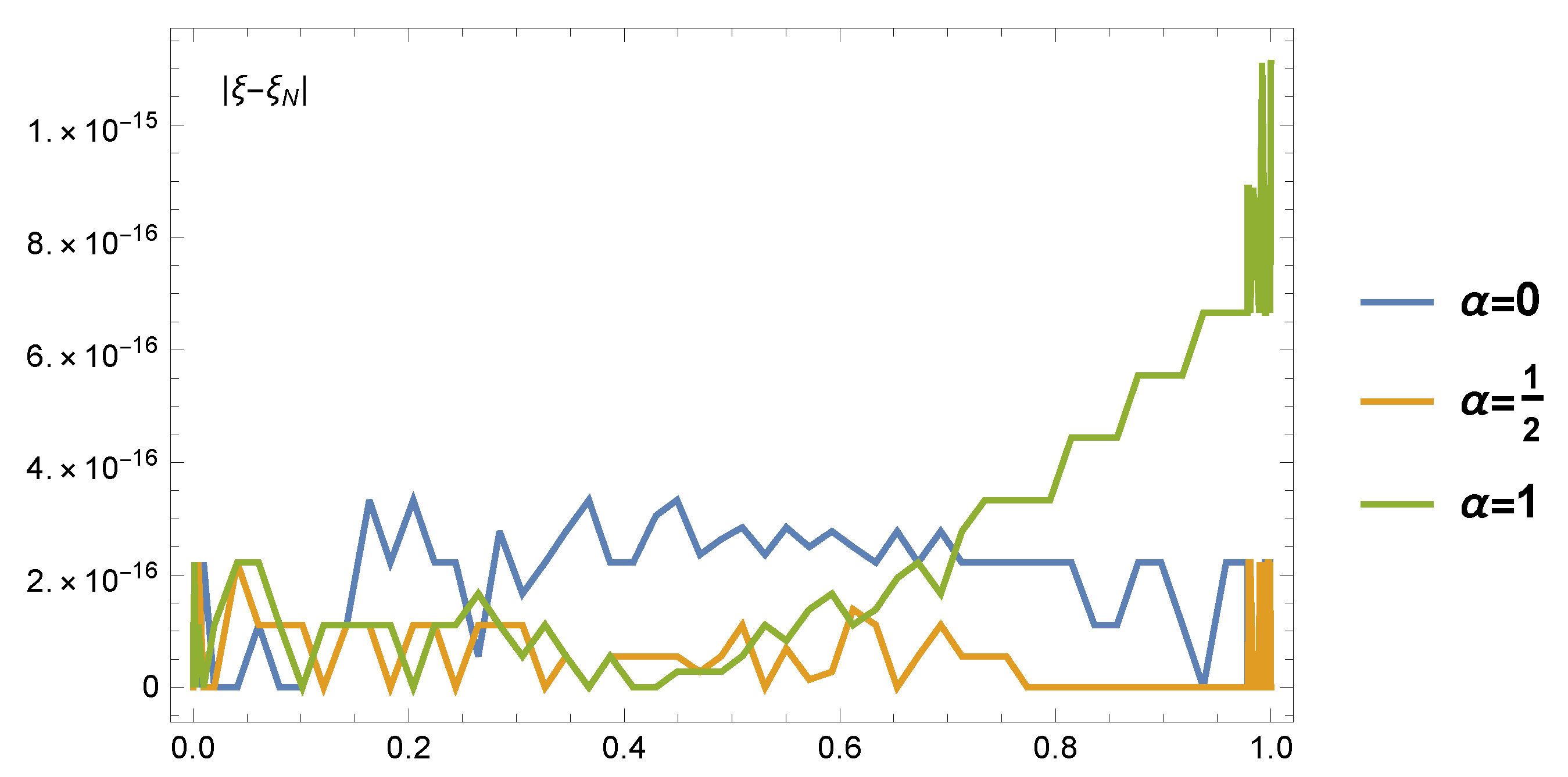
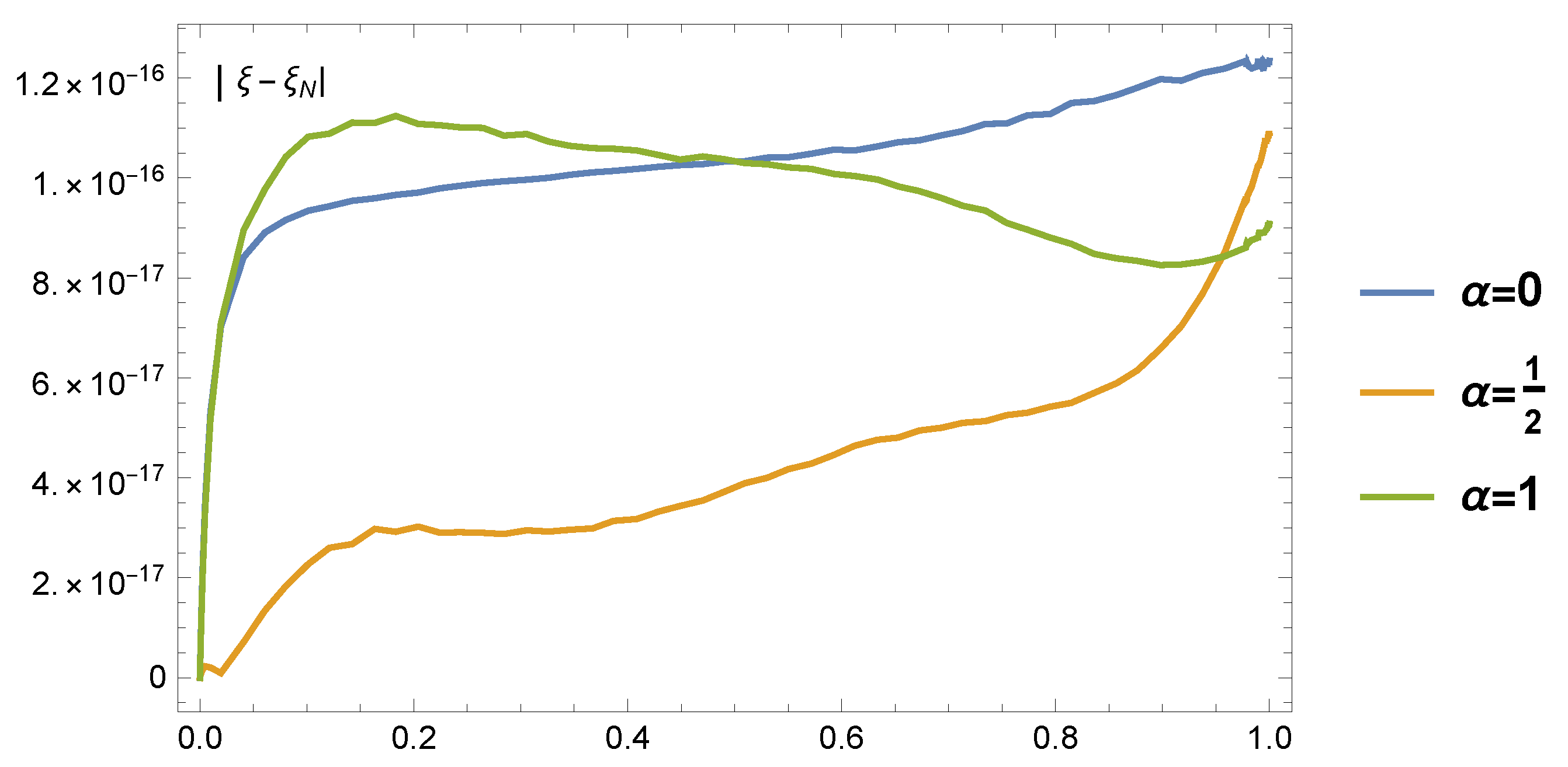
6.2. Numerical Tests

Now, we give two numerical examples accompanied by some comparisons to show the effectiveness and applicability of the proposed ultraspherical tau method ($UTM$).

Example 1.

Consider the non-linear Riccati differential Equation ([9,48,49,50,51]):

$${\xi }^{\prime }\left(x\right)=1+2\xi \left(x\right)-\xi {\left(x\right)}^2,x\in [0,1],\xi \left(0\right)=0,$$

(75)

with the following exact solution:

$$\xi \left(x\right)=\sqrt{2}tanh\left(\sqrt{2}x-{tanh}^{-1}\left(\frac{1}{\sqrt{2}}\right)\right)+1.$$

In

Table 1. Maximum absolute error E for Example 1 ($\alpha =\frac{1}{2})$.

N	6	8	10	12	14	16
E	2.358 × ${10}^{-6}$	3.264 × ${10}^{-7}$	6.382 × ${10}^{-10}$	5.943 × ${10}^{-13}$	2.975 × ${10}^{-15}$	6.241 × ${10}^{-16}$

, the maximum absolute error E is listed for various values of N and for $\alpha =\frac{1}{2}$. Furthermore,

Table 2. Comparison between different methods for Example 1.

x	OHAM [48]	MHPM [49]	VIM [50]	IRKHSM [51]	The Method in [9]	$\mathit{UTM}(\mathit{N}=$$16,\mathit{\alpha }=\frac{1}{2})$
0	0	0	0	0	0	0
0.1	3.20 $\times {10}^{-5}$	1.00 $\times {10}^{-6}$	1.98 $\times {10}^{-8}$	3.58 $\times {10}^{-5}$	1.52 $\times {10}^{-15}$	1.27 $\times {10}^{-17}$
0.2	2.90 $\times {10}^{-4}$	1.20 $\times {10}^{-5}$	1.03 $\times {10}^{-6}$	7.58 $\times {10}^{-5}$	1.27 $\times {10}^{-15}$	2.23 $\times {10}^{-17}$
0.3	1.10 $\times {10}^{-3}$	1.00 $\times {10}^{-6}$	8.85 $\times {10}^{-6}$	1.20 $\times {10}^{-4}$	2.57 $\times {10}^{-15}$	1.34 $\times {10}^{-16}$
0.4	2.50 $\times {10}^{-3}$	3.03 $\times {10}^{-4}$	3.33 $\times {10}^{-5}$	1.66 $\times {10}^{-4}$	3.27 $\times {10}^{-15}$	2.31 $\times {10}^{-16}$
0.5	4.40 $\times {10}^{-3}$	1.55 $\times {10}^{-3}$	7.26 $\times {10}^{-5}$	2.12 $\times {10}^{-4}$	3.57 $\times {10}^{-15}$	3.68 $\times {10}^{-16}$
0.6	5.50 $\times {10}^{-3}$	4.69 $\times {10}^{-3}$	9.98 $\times {10}^{-5}$	2.52 $\times {10}^{-4}$	4.15 $\times {10}^{-15}$	4.32 $\times {10}^{-16}$
0.7	5.50 $\times {10}^{-3}$	1.05 $\times {10}^{-2}$	8.84 $\times {10}^{-5}$	2.87 $\times {10}^{-4}$	4.21 $\times {10}^{-15}$	4.95 $\times {10}^{-16}$
0.8	3.80 $\times {10}^{-3}$	1.88 $\times {10}^{-2}$	1.54 $\times {10}^{-5}$	3.40 $\times {10}^{-4}$	4.31 $\times {10}^{-15}$	5.62 $\times {10}^{-16}$
0.9	3.20 $\times {10}^{-3}$	2.80 $\times {10}^{-2}$	4.99 $\times {10}^{-4}$	4.90 $\times {10}^{-4}$	4.35 $\times {10}^{-15}$	5.94 $\times {10}^{-16}$
1.0	3.40 $\times {10}^{-3}$	3.43 $\times {10}^{-2}$	3.47 $\times {10}^{-3}$	9.22 $\times {10}^{-4}$	4.42 $\times {10}^{-15}$	6.24 $\times {10}^{-16}$

illustrates a comparison between the errors resulting from the application of our algorithm for the case corresponding to $N=16$ and $\alpha =\frac{1}{2}$ with the best errors obtained by the application of the following four methods:

• Optimal homotopy asymptotic method (OHAM) [48],
• Modified homotopy perturbation method (MHPM) [49],
• Variational iteration method (VIM) [50],
• Iterative reproducing kernel Hilbert space method (IRKHSM) [51],
• The method in [9].

The errors are calculated at $x_i=0.1i,0\le i\le 10$. The findings of Table 2 demonstrate that our method is extremely accurate when compared to the above-mentioned methods. The generated numerical solutions are in good agreement with the precise one when just a few of the retained modes are used. In addition, different errors of Example 1 for different values of α are displayed in Figure 1.

Example 2.

Consider the non-linear Riccati differential Equation [52]:

$${\xi }^{\prime }\left(x\right)=\frac{1}{4}+\frac{x^2}{64}-\frac{1}{4}{\left(\xi \left(x\right)\right)}^2,x\in [0,1],\xi \left(0\right)=1.$$

(76)

The exact solution of (76) is ${\displaystyle \xi \left(x\right)=\frac{x}{4}+\frac{4e^{-\frac{x^2}{16}}}{4+{\int }_0^x{e}^{-\frac{t^2}{16}}dt}}$.

Table 3. Maximum absolute error for Example 2.

N	8	10	12	14	16
$\alpha =0$	3.51 $\times {10}^{-8}$	2.45 $\times {10}^{-9}$	2.39 $\times {10}^{-11}$	5.94 $\times {10}^{-13}$	5.37 $\times {10}^{-16}$
$\alpha =\frac{1}{2}$	1.38 $\times {10}^{-8}$	3.27 $\times {10}^{-10}$	8.36 $\times {10}^{-12}$	4.62 $\times {10}^{-12}$	3.74 $\times {10}^{-16}$
$\alpha =1$	4.58 $\times {10}^{-8}$	3.19 $\times {10}^{-9}$	4.94 $\times {10}^{-11}$	6.84 $\times {10}^{-13}$	2.22 $\times {10}^{-16}$

displays the maximum absolute errors resulting from the application of the $UTM$ for $\alpha =0,\frac{1}{2},1$ and for different values of N. Furthermore, different errors for the cases corresponding to $N=16$ and $\alpha =0,\frac{1}{2},1$ are shown in Figure 2.

Remark 6.

We report here that, the best error obtained by Lakestani and Dehghan is $\mathbf{O}\left({10}^{-9}\right)$, from the results depicted in Figure 2, we have a major superiority with few number of retained modes.

7. Conclusions

In this paper, we have considered two different approaches for solving the linearization problems of Jacobi polynomials. The first approach is based on making use of the moments formulas of the shifted Jacobi polynomials and the unified moments formula for the four kinds of Chebyshev polynomials. This approach enables one to derive new general linearization formulas of some Jacobi polynomials in terms of certain terminating hypergeometric functions of a unit argument. Symbolic algebra serves to simplify the linearization formulas of Jacobi polynomials for certain choices of the involved parameters. We also followed another approach to establish some linearization formulas. This approach depends on employing the connection formula between two different Jacobi polynomials. Again, the presented formulas were expressed in different terminating hypergeometric functions of unit argument. In many cases, and using some well-known reduction formulas or some symbolic computation, the appearing hypergeometric functions can be summed in closed analytical forms. The main advantage of using the moments formulas in establishing the linearization formulas is that this approach can be employed to derive the linearization formulas of different polynomials and not restricted to the Jacobi polynomials. To the best of our knowledge, most of the theoretical results of this paper are new and are very useful. To ensure the importance of the presented formulas, a numerical application is analyzed in detail to solve the non-linear Riccati differential equation with the aid of employing the spectral tau method. The presented numerical results and comparisons showed the high accuracy and applicability to the proposed numerical algorithm. We believe that other types of differential equations can be treated based on utilizing the presented linearization formulas.

References

1. Quintana, Y.; Ramírez, W.; Urieles, A. On an operational matrix method based on generalized Bernoulli polynomials of level m. Calcolo 2018, 55, 1–29. [Google Scholar] [CrossRef]
2. Fitri, S.; Thomas, D.K.; Wibowo, R.B.E. Coefficient inequalities for a subclass of Bazilevič functions. Demonstratio Math. 2020, 53, 27–37. [Google Scholar] [CrossRef]
3. Urieles, A.; Ortega, M.J.; Ramírez, W.; Vega, S. New results on the q-generalized Bernoulli polynomials of level m. Demonstratio Math. 2019, 52, 511–522. [Google Scholar] [CrossRef]
4. Doha, E.H.; Abd-Elhameed, W.M.; Bassuony, M.A. On the coefficients of differentiated expansions and derivatives of Chebyshev polynomials of the third and fourth kinds. Acta Math. Sci. 2015, 35, 326–338. [Google Scholar] [CrossRef]
5. Doha, E.H.; Abd-Elhameed, W.M. On the coefficients of integrated expansions and integrals of Chebyshev polynomials of third and fourth kinds. Bull. Malays. Math. Sci. Soc. 2014, 37, 383–398. [Google Scholar]
6. Abd-Elhameed, W.M.; Alkenedri, A.M. Spectral solutions of linear and nonlinear BVPs using certain Jacobi polynomials generalizing third-and fourth-kinds of Chebyshev polynomials. CMES Comput. Model. Eng. Sci. 2021, 126, 955–989. [Google Scholar]
7. Sánchez-Ruiz, J. Logarithmic potential of Hermite polynomials and information entropies of the harmonic oscillator eigenstates. J. Math. Phys. 1997, 38, 5031–5043. [Google Scholar] [CrossRef] [Green Version]
8. Dehesa, J.S.; Finkelshtdein, A.M.; Sánchez-Ruiz, J. Quantum information entropies and orthogonal polynomials. J. Comput. Appl. Math. 2001, 133, 23–46. [Google Scholar] [CrossRef]
9. Abd-Elhameed, W.M. New formulae between Jacobi polynomials and some fractional Jacobi functions generalizing some connection formulae. Anal. Math. Phys. 2019, 9, 73–98. [Google Scholar] [CrossRef]
10. Abd-Elhameed, W.M. Novel expressions for the derivatives of sixth-kind Chebyshev polynomials: Spectral solution of the non-linear one-dimensional Burgers’ equation. Fractal Fract. 2021, 5, 74. [Google Scholar] [CrossRef]
11. Askey, R.; Gasper, G. Linearization of the product of Jacobi polynomials. III. Canad. J. Math. 1971, 23, 332–338. [Google Scholar] [CrossRef]
12. Gasper, G. Linearization of the product of Jacobi polynomials. I. Canad. J. Math. 1970, 22, 171–175. [Google Scholar] [CrossRef]
13. Gasper, G. Linearization of the product of Jacobi polynomials. II. Canad. J. Math. 1970, 22, 582–593. [Google Scholar] [CrossRef]
14. Hylleraas, E.A. Linearization of products of Jacobi polynomials. Math. Scan. 1962, 10, 189–200. [Google Scholar] [CrossRef] [Green Version]
15. Rahman, M. A non-negative representation of the linearization coefficients of the product of Jacobi polynomials. Canad. J. Math. 1981, 33, 915–928. [Google Scholar] [CrossRef]
16. Sánchez-Ruiz, J.; Dehesa, J.S. Some connection and linearization problems for polynomials in and beyond the Askey scheme. J. Comput. Appl. Math. 2001, 133, 579–591. [Google Scholar] [CrossRef]
17. Chaggara, H.; Koepf, W. On linearization coefficients of Jacobi polynomials. Appl. Math. Lett. 2010, 23, 609–614. [Google Scholar] [CrossRef] [Green Version]
18. Srivastava, H.M. A unified theory of polynomial expansions and their applications involving Clebsch-Gordan type linearization relations and Neumann series. Astrophys. Space Sci. 1988, 150, 251–266. [Google Scholar] [CrossRef]
19. Srivastava, H.M.; Niukkanen, A.W. Some Clebsch-Gordan type linearization relations and associated families of Dirichlet integrals. Math. Comput. Model. 2003, 37, 245–250. [Google Scholar] [CrossRef]
20. Niukkanen, A.W. Clebsch-Gordan-type linearisation relations for the products of Laguerre polynomials and hydrogen-like functions. J. Phy. A Math. Gen. 1985, 18, 1399. [Google Scholar] [CrossRef]
21. Kim, T.; Kim, D.S.; Lee, H.; Kwon, J. Studies in sums of finite products of the second, third, and fourth kind Chebyshev polynomials. Mathematics 2020, 8, 210. [Google Scholar] [CrossRef] [Green Version]
22. Dolgy, D.V.; Kim, D.S.; Kim, T.; Kwon, J. Connection problem for sums of finite products of Chebyshev polynomials of the third and fourth kinds. Symmetry 2018, 10, 617. [Google Scholar] [CrossRef] [Green Version]
23. Kim, T.; Kim, D.S.; Dolgy, D.V.; Park, J.W. Sums of finite products of Legendre and Laguerre polynomials. Adv. Differ. Equ. 2018, 2018, 277. [Google Scholar] [CrossRef]
24. Kim, T.; Kim, D.S.; Jang, L.C.; Dolgy, D.V. Representing by several orthogonal polynomials for sums of finite products of Chebyshev polynomials of the first kind and Lucas polynomials. Adv. Difference Equ. 2019, 2019, 162. [Google Scholar] [CrossRef]
25. Kim, T.; Kim, D.S.; Jang, L.C.; Jang, G.W. Fourier series for functions related to Chebyshev polynomials of the first kind and Lucas polynomials. Mathematics 2018, 6, 276. [Google Scholar] [CrossRef] [Green Version]
26. Kim, D.S.; Dolgy, D.V.; Kim, D.; Kim, T. Representing by orthogonal polynomials for sums of finite products of Fubini polynomials. Mathematics 2019, 7, 319. [Google Scholar] [CrossRef] [Green Version]
27. Kim, D.S.; Kim, T. On sums of finite products of balancing polynomials. J. Comput. Appl. Math. 2020, 377, 112913. [Google Scholar] [CrossRef]
28. Doha, E.H.; Abd-Elhameed, W.M. New linearization formulae for the products of Chebyshev polynomials of third and fourth kinds. Rocky Mountain J. Math. 2016, 46, 443–460. [Google Scholar] [CrossRef]
29. Abd-Elhameed, W.M.; Doha, E.H.; Ahmed, H.M. Linearization formulae for certain Jacobi polynomials. Ramanujan J. 2016, 39, 155–168. [Google Scholar] [CrossRef]
30. Abd-Elhameed, W.M. New product and linearization formulae of Jacobi polynomials of certain parameters. Integral Transforms Spec. Funct. 2015, 26, 586–599. [Google Scholar] [CrossRef]
31. Abd-Elhameed, W.M. New formulas for the linearization coefficients of some nonsymmetric Jacobi polynomials. Adv. Differ. Equ. 2015, 2015, 168. [Google Scholar] [CrossRef] [Green Version]
32. Sánchez-Ruiz, J. Linearization and connection formulae involving squares of Gegenbauer polynomials. Appl. Math. Lett. 2001, 14, 261–267. [Google Scholar] [CrossRef] [Green Version]
33. Abd-Elhameed, W.M. New formulae of squares of some Jacobi polynomials via hypergeometric functions. Hacet. J. Math. Stat. 2017, 46, 165–176. [Google Scholar] [CrossRef]
34. Abd-Elhameed, W.M.; Badah, B.M. New specific and general linearization formulas of some classes of Jacobi polynomials. Mathematics 2021, 9, 74. [Google Scholar] [CrossRef]
35. Srivastava, H.M. Some Clebsch-Gordan type linearisation relations and other polynomial expansions associated with a class of generalised multiple hypergeometric series arising in physical and quantum chemical applications. J. Phys. A Math. Gen. 1988, 21, 4463. [Google Scholar] [CrossRef]
36. Ahmed, H.M. Computing expansions coefficients for Laguerre polynomials. Integral Transform Spec. Funct. 2020. [Google Scholar] [CrossRef]
37. Abd-Elhameed, W.M.; Youssri, Y.H. Neoteric formulas of the monic orthogonal Chebyshev polynomials of the sixth-kind involving moments and linearization formulas. Adv. Difference Equ. 2021, 2021, 84. [Google Scholar] [CrossRef]
38. Markett, C. Linearization of the product of symmetric orthogonal polynomials. Constr. Approx. 1994, 10, 317–338. [Google Scholar] [CrossRef]
39. Popov, B.S.; Srivastava, H.M. Linearization of a product of two polynomials of different orthogonal systems. Facta Univ. Ser. Math. Inform 2003, 18, 1–8. [Google Scholar]
40. Olver, F.W.; Lozier, D.W.; Boisvert, R.F.; Clark, C.W. NIST Handbook of Mathematical Functions Hardback and CD-ROM; Cambridge University Press: Cambridge, UK, 2010. [Google Scholar]
41. Andrews, G.E.; Askey, R.; Roy, R. Special Functions; Cambridge University Press: Cambridge, UK, 1999. [Google Scholar]
42. Rainville, E.D. Special Functions; The Maximalan Company: New York, NY, USA, 1960. [Google Scholar]
43. Doha, E.H.; Abd-Elhameed, W.M.; Ahmed, H.M. The coefficients of differentiated expansions of double and triple Jacobi polynomials. Bull. Iranian Math. Soc. 2012, 38, 739–765. [Google Scholar]
44. Mason, J.C.; Handscomb, D.C. Chebyshev Polynomials; Chapman and Hall: New York, NY, USA; CRC: Boca Raton, FL, USA, 2003. [Google Scholar]
45. Koepf, W. Hypergeometric Summation: An Algorithmic Approach to Summation and Special Function Identities, 2nd ed.; Springer Universitext; Springer: London, UK, 2014. [Google Scholar]
46. Van Hoeij, M. Finite singularities and hypergeometric solutions of linear recurrence equations. J. Pure Appl. Algebra 1999, 139, 109–131. [Google Scholar] [CrossRef] [Green Version]
47. Doha, E.H.; Abd-Elhameed, W.M. Efficient spectral-Galerkin algorithms for direct solution of second-order equations using ultraspherical polynomials. SIAM J. Sci. Comput. 2002, 24, 548–571. [Google Scholar] [CrossRef]
48. Mabood, F.; Ismail, A.; Hashim, I. Application of optimal homotopy asymptotic method for the approximate solution of Riccati equation. Sains Malays. 2013, 42, 863–867. [Google Scholar]
49. Odibat, Z.; Momani, S. Modified homotopy perturbation method: Application to quadratic Riccati differential equation of fractional order. Chaos Solitons Fractals 2008, 36, 167–174. [Google Scholar] [CrossRef]
50. Batiha, B.; Noorani, M.S.M.; Hashim, I. Application of variational iteration method to a generalRiccati equation. Int. Math. Forum 2007, 2, 2759–2770. [Google Scholar] [CrossRef] [Green Version]
51. Sakar, M. Iterative reproducing kernel Hilbert spaces method for Riccati differential equations. J. Comput. Appl. Math. 2017, 309, 163–174. [Google Scholar] [CrossRef]
52. Lakestani, M.; Dehghan, M. Numerical solution of Riccati equation using the cubic B-spline scaling functions and Chebyshev cardinal functions. Comput. Phys. Commun. 2010, 181, 957–966. [Google Scholar] [CrossRef]
Figure 1. Different errors of Example 1 for different values of α.
Mathematics 09 01573 g001
Figure 2. Different errors of Example 2 for different values of α.
Mathematics 09 01573 g002