Acceleration of Boltzmann Collision Integral Calculation Using Machine Learning

Abstract

The Boltzmann equation is essential to the accurate modeling of rarefied gases. Unfortunately, traditional numerical solvers for this equation are too computationally expensive for many practical applications. With modern interest in hypersonic flight and plasma flows, to which the Boltzmann equation is relevant, there would be immediate value in an efficient simulation method. The collision integral component of the equation is the main contributor of the large complexity. A plethora of new mathematical and numerical approaches have been proposed in an effort to reduce the computational cost of solving the Boltzmann collision integral, yet it still remains prohibitively expensive for large problems. This paper aims to accelerate the computation of this integral via machine learning methods. In particular, we build a deep convolutional neural network to encode/decode the solution vector, and enforce conservation laws during post-processing of the collision integral before each time-step. Our preliminary results for the spatially homogeneous Boltzmann equation show a drastic reduction of computational cost. Specifically, our algorithm requires $O(n^3)$ operations, while asymptotically converging direct discretization algorithms require $O(n^6)$, where n is the number of discrete velocity points in one velocity dimension. Our method demonstrated a speed up of 270 times compared to these methods while still maintaining reasonable accuracy.

1. Introduction

While the Euler and Navier–Stokes equations have for a long time been the work horses in the modeling of fluid dynamics, these equations are inadequate for modeling complex flows, such as rarefied gases, for which the continuum assumption is invalid. Rarefied gas flows have become a topic of increasing interest due to their relevance in practical applications such as hypersonic and space vehicles. To accurately capture the true physics of these non-equilibrium flows, analysis of molecular-level interactions is required. As the governing equation of kinetic theory, the Boltzmann equation is key in understanding these interactions, and therefore also critical in aiding the successful design of these flight vehicles, as well as other applications. Unfortunately, and despite the rapid increase in computing power of recent years, numerical solution of this equation continues to present a major challenge. Among the components of the equation, the main driver of computational complexity is the multi-dimensional collision integral. As a result, a plethora of new mathematical and numerical approaches have been proposed in an effort to reduce the computational cost of solving the Boltzmann collision integral.

Fourier-based spectral methods represent a potent approach to deterministic evaluation of the collision integral [1,2,3,4,5]. These methods use uniform meshes in the velocity space and have complexity of $O(n^6)$ operations, where n is the number of discrete velocity points in one velocity dimension. A discontinuous Galerkin discretization with $O(n^6)$ complexity was proposed in [6]. While these algorithms are suitable for simulation of flows in one and two spatial dimensions, they are difficult to use for three dimensional flows. An additional reduction in complexity is achieved in fast spectral methods by leveraging low rank approximate diagonalization of the weighted convolution form of the collision integral [7,8,9,10,11]. Complexities of the fast spectral methods may vary between $O(M_r{M}^2{n}^{3}logn)$ and $O(M^2{n}^{3}logn)$ depending on the form of molecular interaction potential. Numbers $M^2$ and $M_r$ correspond to the numbers of discrete integration points in angular and radial directions used in diagonalization and usually are significantly smaller than n. In spite of the significant improvement in efficiency, simulation of three dimensional flows of gases with internal energies, multi-component gases, and flows in complex geometries still remains challenging for fast spectral methods.

Other algorithms of lower complexities have also been proposed for either special physics or various representations of the approximate solutions, for example, $O(n^4)$ algorithm for evaluating the collision integral in the case of Maxwell’s pseudo-molecules [12], and $O(M{n}^{3}logn)$ for hard spheres potentials [13,14]. Simulation of gas mixtures and gases with internal energies, as well as multidimensional models can be found in [14,15,16,17,18,19,20], and references therein. Other fast methods include representing the solution as a sum of homogeneous Gaussians [21,22], polynomial spectral discretization [23], utilizing non-uniform meshes [24], and a hyperbolic cross approximation [25]. Additional review of recent results can be found in [26,27].

In this paper, we apply machine learning to accelerate the calculation of the Boltzmann collision integral. The results presented are intended to be an initial demonstration of the viability of machine learning to accelerate solution of the problem at hand, more so than to rigorously prove consistency of machine learning techniques with the discretized Boltzmann equation. For our case study, we consider a class of solutions to the problem of spatially homogeneous relaxation computed using deterministic approach of [6]. The considered class of solutions correspond to hard spheres potential, however, we expect that the results can be replicated for other molecular potentials. We build a deep convolutional neural network to encode/decode the solution vector, and enforce conservation laws during post-processing of the collision integral before each time-step. Our preliminary results for the spatially homogeneous Boltzmann equation show a drastic reduction of computational cost, in the order of $O(n^3)$, compared to $O(n^6)$ for direct discretization algorithm of [6].

Specifically, our model would take the numerical solution as input and return a predicted collision integral at every point of the computational domain as output. This model could then directly replace the collision integral calculation in a time stepping simulation without requiring any other aspect of the simulation to change. Due to the fact that machine learning algorithms are to be trained on a specific set of data, the resulting approximate algorithms will be only applicable to the same classes of problem for which the data was generated. Thus, the proposed approaches are intrinsically applicable to a specific set of problems. For that set of problems, however, the methods provide a significant improvement in speed compared to classical methods. This opens an entire new avenue for addressing the computational complexity associated with solving the Boltzmann equation.

Artificial neural networks and machine learning were previously applied to solution of partial differential equations, see, e.g., [28,29,30], including solution of kinetic equations [31]. Another data driven approach consists of using low rank tensor approximations of kinetic solutions [32]. Commonly, deep neural networks provide low rank representations of solutions in high dimensional spaces while the governing partial differential equations are used to define penalty functions for network training. It should be noted, however, that a direct implementation of the collision integral in a penalty function in a manner the governing equations are used in physics informed networks, is problematic due to extremely high costs of evaluating the collision integral. As a result, in this paper, we focus on learning the collision operator itself, for a class of solutions. The resulting approximation can be, in principle, combined with approaches of [31,32] to provide an inexpensive physically accurate collision operator. To the authors’ knowledge, this is the first attempt at using machine learning to accelerate the calculation of the Boltzmann collision integral. Our early results suggest that the approach has potential to drastically advance the state-of-the-art in simulating complex flows or rarefied gas.

The rest of the paper is organized as follows. Section 2 presents the problem setup and the convolutional network structure that enables the dimension reduction. Conservation considerations are described in Section 3. Section 4 is devoted to error analysis. Our test models and results are shown in Section 5. The paper is concluded in Section 6.

2. Problem Setup

In the kinetic approach the gas is described using the molecular velocity distribution function $f(t,\overrightarrow{x},\overrightarrow{v})$ which has the property that $f(t,\overrightarrow{x},\overrightarrow{v})d\overrightarrow{x}d\overrightarrow{v}$ represents the number of molecules that are contained in the box with the volume $d\overrightarrow{x}$ around point $\overrightarrow{x}$ whose velocities are contained in a box of volume $d\overrightarrow{v}$ around point $\overrightarrow{v}$. In this work, we are concerned with the solution of the spatially homogeneous flows that correspond to the assumption that the $f(t,\overrightarrow{x},\overrightarrow{v})$ is constant in the $\overrightarrow{x}$ variable. In this case, the dynamics of the gas is given by the spatially homogeneous Boltzmann Equation (see, for example [33,34]),

$$\frac{\partial }{\partial t}f(t,\overrightarrow{v})=I[f](t,\overrightarrow{v}).$$

(1)

Here $I[f]$ is the molecular collision operator

$$I[f](t,\overrightarrow{x},\overrightarrow{v})={\int }_{{\mathbb{R}}^3}{\int }_{{\mathbb{S}}^2}(f(t,{\overrightarrow{v}}^{\prime })f(t,{\overrightarrow{u}}^{\prime })-f(t,\overrightarrow{v})f(t,\overrightarrow{u}))B(|g|,cos\theta )d\sigma d\overrightarrow{u},$$

(2)

where $\overrightarrow{v}$ and $\overrightarrow{u}$ are the pre-collision velocities of a pair of particles, $\overrightarrow{g}=\overrightarrow{v}-\overrightarrow{u}$, ${\mathbb{S}}^2$ is a unit sphere in ${\mathbb{R}}^3$ centered at the origin, $\overrightarrow{w}$ is the unit vector connecting the origin and a point on ${\mathbb{S}}^2$, $\theta$ is the deflection angle defined by the equation $cos\theta =\overrightarrow{w}·\overrightarrow{g}/|g|$, $d\sigma =sin\theta d\theta d\epsilon$, where $\epsilon$ is the azimuthal angle that parametrizes $\overrightarrow{w}$ together with the angle $\theta$. Vectors ${\overrightarrow{v}}^{\prime }$ and ${\overrightarrow{u}}^{\prime }$ are the post-collision velocities of a pair of particles and are computed by

$${\overrightarrow{v}}^{\prime }=\overrightarrow{v}-\frac{1}{2}(\overrightarrow{g}-|g|\overrightarrow{w}),{\overrightarrow{u}}^{\prime }=\overrightarrow{v}-\frac{1}{2}(\overrightarrow{g}+|g|\overrightarrow{w}).$$

Due to the high computational complexity of the collision integral, use of the Boltzmann equation in practice has been limited.

2.1. Class of Solutions and Solution Collection

The class of solutions for which the training data is constructed consists of solutions to the problem of spatially homogeneous relaxation with the initial data given by two homogeneous Gaussian densities. The initial data is normalized so that the velocity distribution function has unit density, zero bulk velocity and, a set temperature. In the simulations presented in this paper, the value of dimensionless temperature of 0.2 was used. The bulk velocities of the homogeneous Gaussian densities have zero v and w components, thus the solutions are radially symmetric in $vw$ velocity plane.

A collection of solutions is computed by randomly generating macroscopic parameters of density, the u components of the bulk velocity, and temperatures of two homogeneous Gaussian densities and solving (1) until a steady state is reached using the method of [6]. The numerically computed velocity distribution functions are saved at multiple instances in time, each save becoming a data point in the collection. We note that due to normalization of the initial data, the steady state is the same for all computed solutions. All solutions were computed on uniform meshes with dimensions of 41 by 41 by 41 in the velocity domain.

2.2. Dimension Reduction

A key component of finding a faster method of calculating the collision integral is finding low dimensional features that adequately characterize the solution. The true dimensionality of the solution data can be demonstrated using the SVD decomposition. The saved solutions are re-arranged as one dimensional arrays $f_j$. Then $f_j$ are added as rows to the matrix $D_{ij}$, where index i runs over all saved solutions and index j runs over all discretization points. This process is schematically depicted in Figure 1.

In Figure 1, singular values of matrix $D_{ij}$, $i=1,\dots ,P$, $j=1,\dots ,M^3$ are shown, where $M=41$ is the number of velocity points in each velocity dimension in the computed solutions and P is the total number of the considered solution saves, $P\approx 5000$. About 100 of cases of initial data is included in the results in Figure 1. It can be seen that the singular values decrease very fast allowing for low rank approximation ${\widehat{D}}_{ij}$ of the data matrix $D_{ij}$:

$${\widehat{D}}_{ij}=\sum _{l=1}^K{\sigma }_l{\mu }_i^l{\xi }_j^l.$$

(3)

Here ${\sigma }_l$ is the l-th singular value, ${\mu }_i^l$ is the l-th left singular vector and ${\xi }_j^l$ is the l-th right singular vector of $D_{ij}$. Vectors ${\xi }_j^l$ represent orthogonal modes in solutions and ${\sigma }_l$ represents the relative importance of these modes in the solution data. A SVD truncation theorem of numerical linear algebra states that the relative $L^2$ norm of error of approximating $D_{ij}$ with a truncated sum (3) is $0.001$ for $K=21$ and $1.0\times {10}^{-4}$ for $K=38$. The relative $L^{\infty }$ norm of the SVD truncation error is often estimated using the quantity $e_K=({\sum }_{i=K+1}^P{\sigma }_i)/{\sum }_{i=1}^P{\sigma }_i$. Values of $e_K$ for $K=20$, $K=36$, and $K=55$ are $0.0087$, $0.00089$, and $9.8\times {10}^{-5}$, respectively. This suggests that modes corresponding to singular values ${\sigma }_l$, $l>20$ account for less than $0.01$ of the solutions, for $l>36$ for less than 0.001, and for $l>55$ for less than $1.0\times {10}^{-4}$ of the solutions. In other words, the solutions can be approximated accurately with first 55 singular vectors ${\xi }_j^l$ and these vectors provide a very efficient basis for representing this class of solutions (but not other classes of solutions).

To assess the ability of low rank features to be learned, experiments were conducted applying autoencoders to solution data. An autoencoder is a type of neural network which tries to learn a compressed form of the data on which it is trained. Such a network will contain a constricted layer with only a few output nodes which is meant to be the compressed data. The layers preceding this bottleneck are referred to as the encoder and the layers following are the decoder.

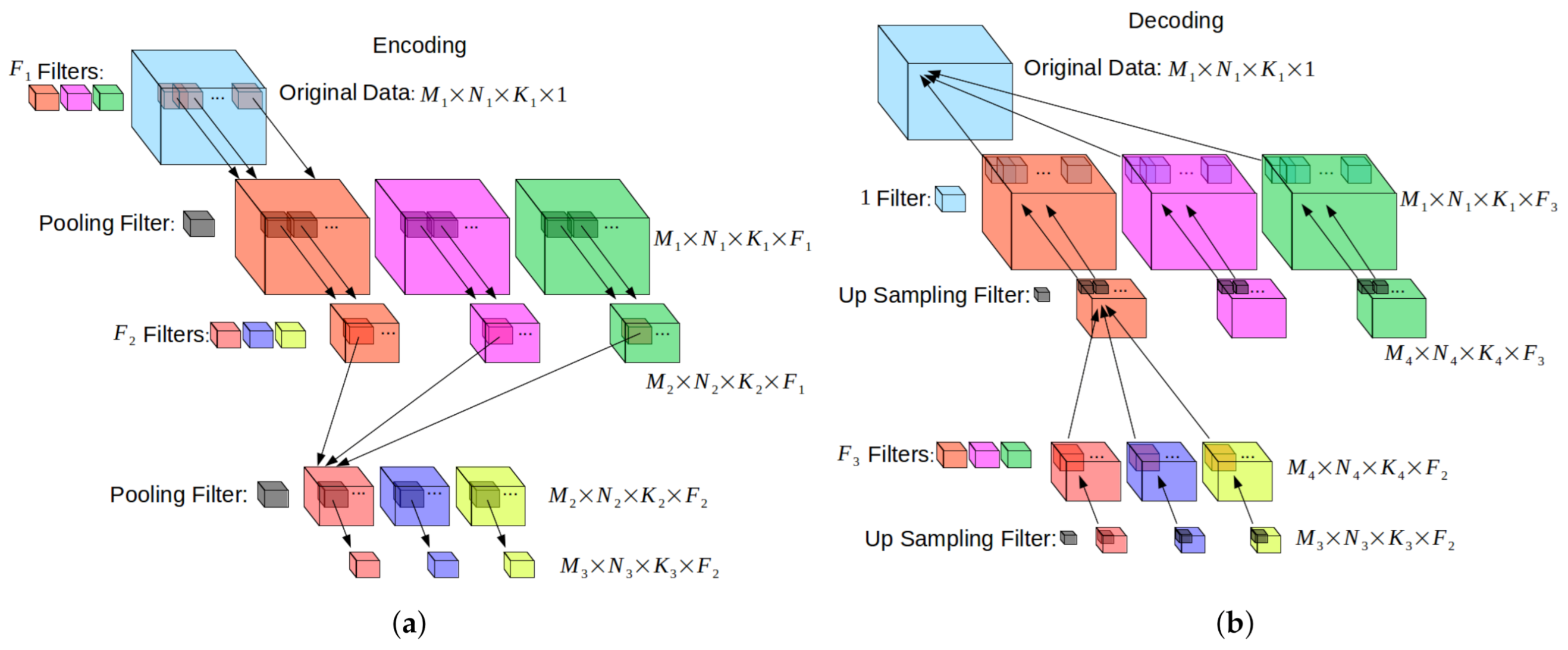
The architecture of autoencoders applied involved convolutional layers, thus making them convolutional autoencoders. As with much of machine learning, there is no specific way that such a network must be constructed. Generally speaking, a 3D convolutional autoencoder will have an encoder with layers arranged as depicted in Figure 2a, and a decoder with layers as depicted in Figure 2b. Figure 2a shows three convolutional filters being applied to the original, resulting in the next three data blocks (color coded to match). These data blocks are then reduced in size by the application of a pooling filter. Another round of convolutional filters is applied, followed by another pooling filter. In Figure 2b, that process is occurring in reverse. The three small data blocks in the beginning are up-sampled to increase their size, then go through a set of convolutional filters. This result is up-sampled again before a final convolutional filter returns the data block to its original dimensions.

The goal is for the convolutional layers to learn key features in the data which are sufficient to reconstruct the data but can be stored in a smaller dimensional space. The compression and decompression is controlled by pooling and upsampling layers. Pooling layers such as max pooling or average pooling replace a block of values in the data with a single value (the max or the average, respectively) which reduces the total number of values being handled. Upsampling layers do the opposite which is to increase the number of values being handled by either repeating values or inserting values which interpolate neighboring values. Alternatively, a network can be allowed to learn its own up-sampling method using transposed convolutional layers.

The convolutional layers are inserted between the pooling and upsampling layers to do the learning. The size of the kernels being applied as well as their activation functions and the number of filters applied are all hyperparameters which must be chosen to get the best results. The requirement for an autoencoder is that at the bottleneck, the number of filters must be such that the total number of values being output is less than the number of values at the input to the network. In Figure 2a this means that $M_3\times N_3\times K_3\times F_2\ll M_1\times N_1\times K_1$.

Samples of the data were taken randomly from the database without discriminating based on initial conditions or the time at which the solution was saved to construct training and test sets. A few different network architectures were constructed and fit to the data using the Keras API included with TensorFlow [35]. The Nadam optimizer proved most effective at training the models. Compared to the Adam and Stochastic Gradient Descent optimizers, Nadam converged the fastest and resulted in the lowest prediction error. A variety of hyperparameter values were explored for the training, some results of this exploration are discussed next.

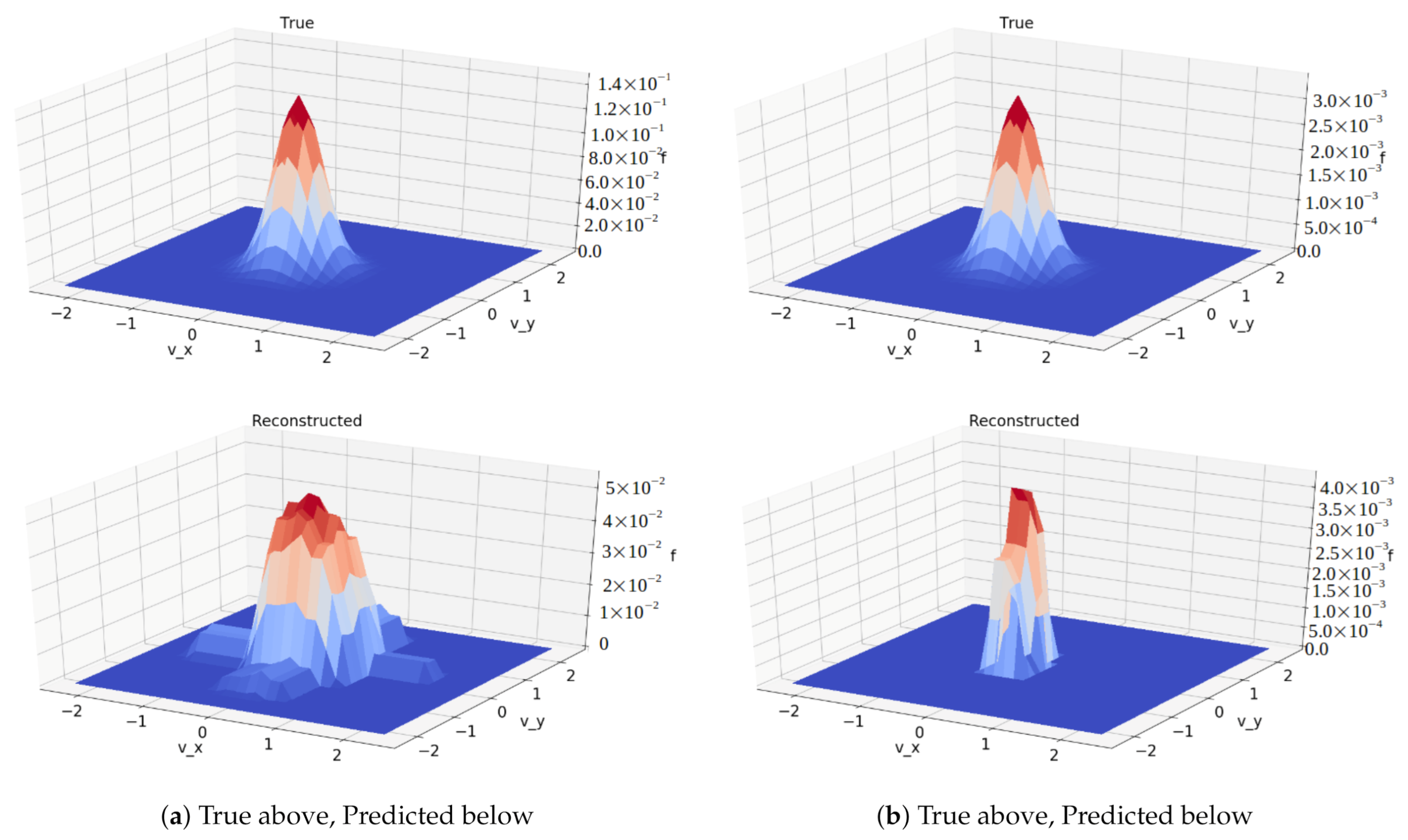
To demonstrate the performance of the autoencoders, we provide some graphs of the reconstructed solutions to compare to the original solutions. The solutions are 3D data cubes and so can not be easily plotted in totality. Instead we have provide graphs of slices of the domain, taken near the center. The results in Figure 3 come from a network with a bottleneck with dimensions of 8 by 8 by 8 with 8 filters which translates to $8^4$ or 4096 variables which is a significant reduction down from ${41}^3$ variables. Both the encoder and decoder portions of the network had three convolutional layers, all of which used the ReLU activation function. The ReLU activation function and its derivative are simple and computationally cheap to use and still grant networks the universal approximator property [36]. Furthermore, we observed ReLU to be easier to train than sigmoid. It has been shown that ReLU is easier to train than sigmoid and sigmoid-like activation functions, because it does not suffer from the vanishing gradient problem [37,38]. Since our autoencoding problem is not a categorical one, the restricted range of sigmoid-like activation functions provides no advantage, and thus ReLU was the preferable activation function.

The results in Figure 4 come from a network with a bottleneck with dimensions of 2 by 2 by 2 with 8 filters which translates to 64 variables. The architecture of this network was identical to the previous, less restricted network, other than the bottleneck being tighter.

The results show promise that the convolutional architecture is capable of identifying and capturing important features in this data set, even with a significantly smaller number of variables. This provides hope that machine learning algorithms will be able to compute such solutions with far less computational effort and memory usage than traditional methods. It is most notable that the peaks of the reconstructed graphs have been rounded off and do not reach as high as the true data. Still captured though is the location and general Maxwellian shape, with the reconstructions from the network with the tighter restriction definitely being lossier than those from the less restricted network.

3. Conservation Laws

Exact solutions to the spatially homogeneous Boltzmann equation must adhere to the conservation of mass, momentum, and energy. Each of these quantities is computed from the solution by the application of a linear integral operator. When these operators are applied to the collision integral, the result must be zero in order to ensure conservation.

The present strategy to enforce conservation laws in numerical solution is to post-process the collision integral after it is predicted and before it is used to step in time as shown in Algorithm 1. Many approaches have been proposed to enforce conservation laws in numerical evaluation of the collision integral, see, e.g., [17,39,40]. In this paper, we employ a modification of the Lagrangian multiplier method of [41,42]. The resulting post-processing procedure is schematically described in Algorithm 2. The procedure computes a corrected value of the collision integral that satisfies the discrete conservation laws up to roundoff errors while being as close as possible to the prediction. The difference from the approach of [42] is that values of the predicted collision integral that are small in magnitude are not affected by the procedure. Thus, the procedure avoids creation of small spurious values in the conservative collision integral at the domain boundaries.

In the future, enforcement of the conservation laws can be incorporated into the model and will thus force the training process to account for them. For example, let M be a 5 by m matrix ($5<m$) which computes the mass, momentum, and energy from the solution. The collision integral must exist in the null space of this matrix. The basis of the null space consists of columns of $V_0$ from the singular value decomposition of the matrix M,

$${\displaystyle M=U[S0]}\left[\begin{array}{c}{V}_1^T\\ V_0^T\end{array}\right]$$

(4)

where U, S are 5 by 5 matrices and $V=[V_1,V_0]$ is an m by m matrix. Thus,

$$Q=\sum _{i=6}^m{\alpha }_i{v}_i,$$

(5)

where

$$V_0=\left[\begin{array}{cccc}{v}_6& v_7& \dots & v_m\end{array}\right].$$

(6)

A model can then be taught to learn values for the parameters $\left\{{\alpha }_i\right\}$ such that Equation (5) approximates the collision integral. This will ensure that the conservation laws are automatically satisfied.

Algorithm 1 Solve 0-dimensional Boltzmann.

1: while$t<t_f$do 2:     Compute $\widehat{Q}=\widehat{Q}[f(t)]$ using machine learned model 3:     $\widehat{Q}=\mathtt{enforceConservation}(\widehat{Q})$ 4:     $f(t+\Delta t)=f(t)+\Delta t\ast \widehat{Q}$ 5: end while

Algorithm 2 Enforce Conservation.

1: procedure enforceConservation(q) 2:       Construct mass, momentum, and energy operator, M 3:       Construct a masking projection operator P that preserves small components of q and nullifies other components 4:       Solve $min\frac{1}{2}||q_{\mathrm{corr}}-q{||}^2$ s.t. $M{q}_{\mathrm{corr}}=0$, $P(q_{\mathrm{corr}}-q)=0$ 5:       return $q_{\mathrm{corr}}$ 6: end procedure

4. Error Propagation

A known weakness of using a machine learned model in place of an analytical one is that errors will be injected into the simulation process. Even if the magnitude of the generated error is small, the way these errors evolve and interact may be significant. It is thus desirable to understand how the errors will behave. In our case, if we define $\widehat{Q}$ as the machine-learned model for the collision integral and $\widehat{f}$ as the solution computed using that model, then we can define the error functions as

$$e_f=f-\widehat{f}$$

(7)

and

$$e_Q=Q[f]-\widehat{Q}[\widehat{f}].$$

(8)

We then have an equation for the evolution of error given by

$$\frac{\partial }{\partial t}{e}_f+\overrightarrow{v}·{\nabla }_x{e}_f=e_Q,$$

(9)

from which we can derive some approximate error bounds.

If one assumes that the distribution of error is approximately uniform, then the second term can be ignored. This leaves

$$\frac{\partial }{\partial t}{e}_f=e_Q.$$

(10)

Writing $e_Q$ as

$$e_Q=\left(Q[f]-\widehat{Q}[f]\right)+\left(\widehat{Q}[f]-\widehat{Q}[\widehat{f}]\right),$$

(11)

we see that there are two contributions to the error. The first is the error in the prediction due to the model not being exact, the second is from error accumulated during the time stepping process. If we now assume Lipschitz continuity of the model and that the prediction error is bounded by a constant, then

$$|e_Q|\le C_1+C_2|f-\widehat{f}|=C_1+C_2|e_f|.$$

(12)

The worst case scenario estimate is

$$\frac{\partial }{\partial t}|e_f|\le C_1+C_2|e_f|,$$

(13)

which leads to the bound on the solution’s error

$$|e_f(t,\overrightarrow{x},\overrightarrow{v})|\le \frac{C_1}{C_2}\left(e^{C_{2}t}-1\right).$$

(14)

Depending on the application for which the Boltzmann equation is being solved, it may not be sufficient just to bound the magnitude of the error in the prediction of the solution, but the effect the error has on the moments may also be of interest. It is from the moments that many physical properties of the gas are computed and the errors in the solution may manifest in ways which significantly or insignificantly affect the moments of the solution. In general, a moment of the solution is given by

$$m_i={\int }_{\Omega }{q}_{i}f,$$

(15)

where $q_i$ is a quantity associated with the definition of the $i$th moment. Therefore, the error in the moment calculation is

$$e_{m_i}={\int }_{\Omega }{q}_{i}f-{\int }_{\Omega }{q}_i\widehat{f}={\int }_{\Omega }{q}_i{e}_f,$$

(16)

which is the corresponding moment of the error. For error in the collision integral prediction satisfying our previous assumptions, the error bound on the moment calculation is

$$|e_{m_i}|\le \frac{C_1}{C_2}(e^{C_{2}t}-1){\int }_{\Omega }|q_i|.$$

(17)

As of yet, it cannot be said what kind of errors should be expected or how they will manifest themselves, other than that the error in the mass, momentum, and energy moments will be exactly zero due to conservation law enforcement. We expect that lower order moments will be less affected by introduced error, however higher order moments could react dramatically to small deviations in the solution.

5. Test Model

Examination of trends in the solution, collision integral pairs in the database led to the conclusion that a second order function should have sufficient flexibility to predict the value at each point of the collision integral. The chosen predictors for each value in the collision integral were the 27 values in the solution in the neighborhood of the index in the collision integral being predicted.

A sparsely connected neural network was then constructed using an expanded feature space which included second order terms computed from the predictors. For a given value in the collision integral, $y_{i^{\ast }{j}^{\ast }{k}^{\ast }}$, at indices $i^{\ast }$, $j^{\ast }$, $k^{\ast }$, let $P_{i^{\ast }{j}^{\ast }{k}^{\ast }}$ be the set of corresponding features which is

$$\begin{array}{cc}\hfill P_{i^{\ast }{j}^{\ast }{k}^{\ast }}\{x_{i_1{j}_1{k}_1},& x_{i_1{j}_1{k}_1}{x}_{i_2{j}_2{k}_2}|\hfill \\ \hfill & d((i_1,j_1,k_1),(i^{\ast },j^{\ast },k^{\ast }))\le 1,d((i_2,j_2,k_2),(i^{\ast },j^{\ast },k^{\ast }))\le 1\},\hfill \end{array}$$

(18)

where $d((i_1,j_1,k_1),(i^{\ast },j^{\ast },k^{\ast }))=max(|i_1-i^{\ast }|,|j_1-j^{\ast }|,|k_1-k^{\ast }|)$. We then define $X_{i^{\ast }{j}^{\ast }{k}^{\ast }}$ to be a vector of all the elements in $P_{i^{\ast }{j}^{\ast }{k}^{\ast }}$. The model to predict $y_{i^{\ast }{j}^{\ast }{k}^{\ast }}$ is the support vector machine,

$$y_{i^{\ast }{j}^{\ast }{k}^{\ast }}=w_{i^{\ast }{j}^{\ast }{k}^{\ast }}^T{X}_{i^{\ast }{j}^{\ast }{k}^{\ast }}+w_{i^{\ast }{j}^{\ast }{k}^{\ast },0},$$

(19)

with parameters $w_{i^{\ast }{j}^{\ast }{k}^{\ast }}$, and $w_{i^{\ast }{j}^{\ast }{k}^{\ast },0}$ which correspond to the given $y_{i^{\ast }{j}^{\ast }{k}^{\ast }}$. The full network made up of these SVMs is a sparsely connected, single layer network with linear activation functions. In total this architecture has $O(n^3)$ parameters and requires $O(n^3)$ flops to compute the collision integral where n is the number of indices along a single dimension of the discrete mesh. Both the computational complexity and memory requirements are this linear in the size of the mesh. The model was fit to training data using a regularized least squares loss function and achieved overall good predictions.

Comparison of Results

To assess the performance of this machine-learned method for computing the collision integral, the model was used to solve the spatially homogeneous Boltzmann equation

$$\frac{\partial }{\partial t}f(t,\overrightarrow{v})=Q[f](t,\overrightarrow{v})$$

(20)

using forward Euler integration in time as shown in Algorithm 1. The solution was integrated starting with initial data $f(0,\overrightarrow{v})$ from the database of solutions.

The Python implementation of this method took about 6 min to carry out 667 time steps and about 9 min to carry out 1000 time steps, an estimated $O({10}^2)$ times faster than the method of [6]. That method uses a discontinuous Galerkin discretization and takes about 40 h on a single CPU to carry out 1000 time steps. The machine-learned method thus greatly outperformed the method of [6]. The CPU time for both methods to perform one evaluation of the collision operator are summarized in

Table 1. Time to perform one evaluation of the collision operator using machine-learned collision operator and the $O(n^6)$ deterministic method of [6].

	ML Method	Deterministic	Speed Up
Time, s	0.54	147	270×

. The CPU time for the machine-learned method also shows significant improvement compared to times reported in [10] for a fast spectral method.

Solutions computed using the machine-learned collision operator were comparable to the deterministic solutions with better predictions towards the center of the domain than towards the boundary. Figure 5 and Figure 6 show comparisons between solutions achieved using the method in [6] and the present method. As was the case with the autoencoder, these plots are of slices of the domain. The predictions look very similar and trend toward the same steady state over time. The fact that the quality of the prediction is better closer to the center of the domain may be a result of the training data being more diverse towards the center of the domain than towards the boundary. The true solution and collision integral go to zero at the boundary of the domain and so there was not as much information to use to train the model out there. Even still, the magnitude of the difference between the prediction and the true value was small.

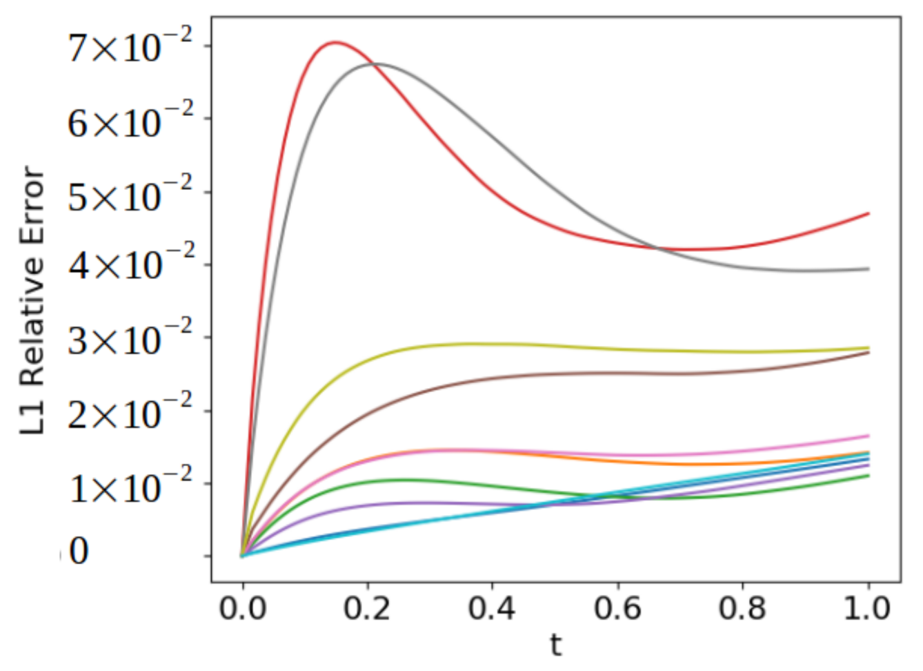
Figure 7 demonstrates how the absolute error between the true solution and the predicted solution evolves over time. The total magnitude of the difference remains low throughout the duration of the simulation, being under 10% of the $L1$ norm of the true solution. There is also a consistent behavior among all the error curves, mainly that the difference grows the most during the first few iterations, then starts to flatten out.

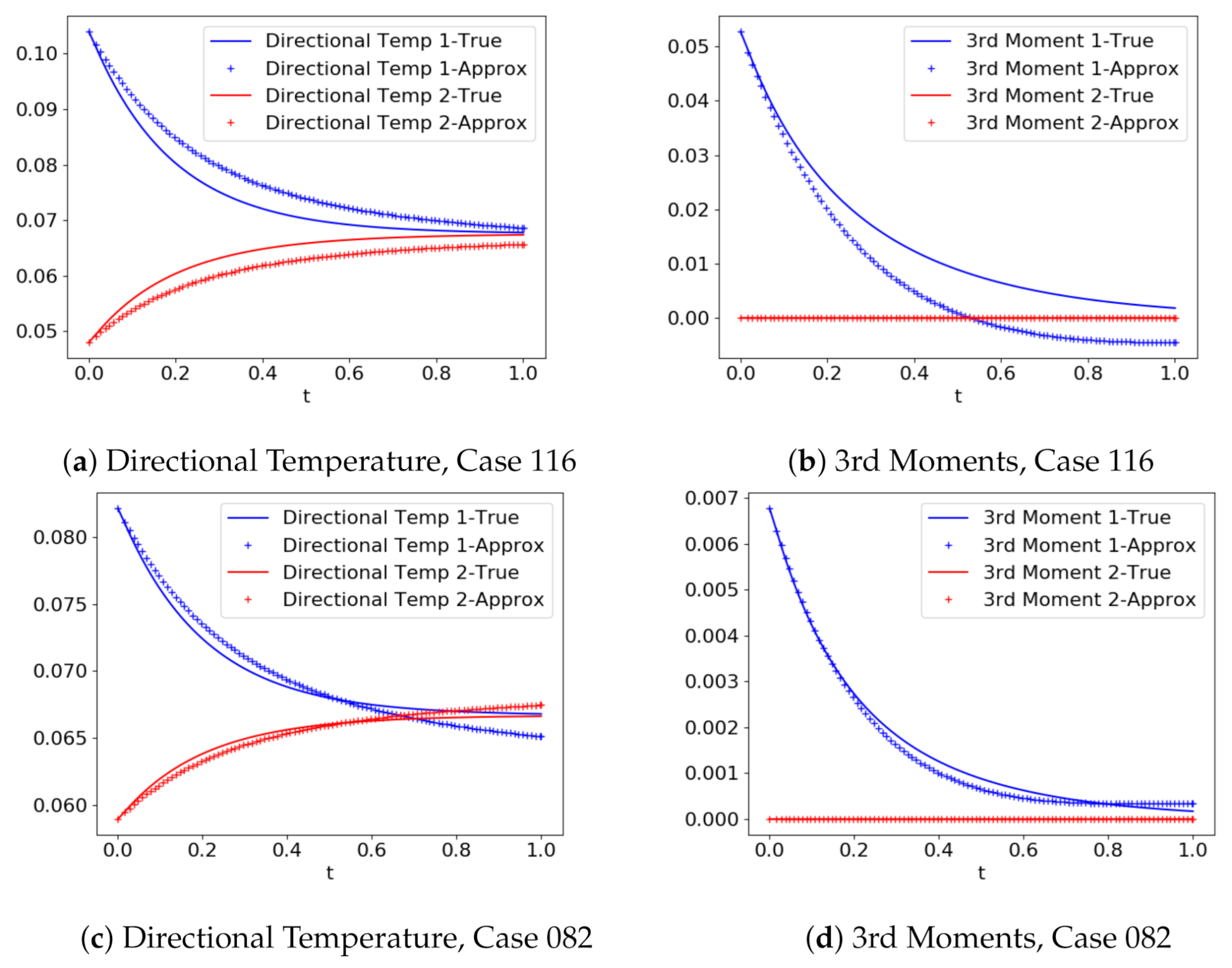
It is now of interest to see the effect the error has on the moments of the solution. Figure 8 shows a comparison of second and third order moments between the predicted and true solution. The lower order moments corresponding to mass, momentum, and temperature moments are not shown because they match exactly with the analytically computed solution’s moments. Generally, the moments of the predicted solutions followed the true moments and headed towards the steady state. They did not however perfectly arrive and remain at the steady state. In some cases the moments of the predicted solution cross over each other, and in other cases they simply fail to meet. The higher order moments exhibited similar behaviors, even more so than the lower order moments, but for many applications moments higher than 3rd order will not be as important.

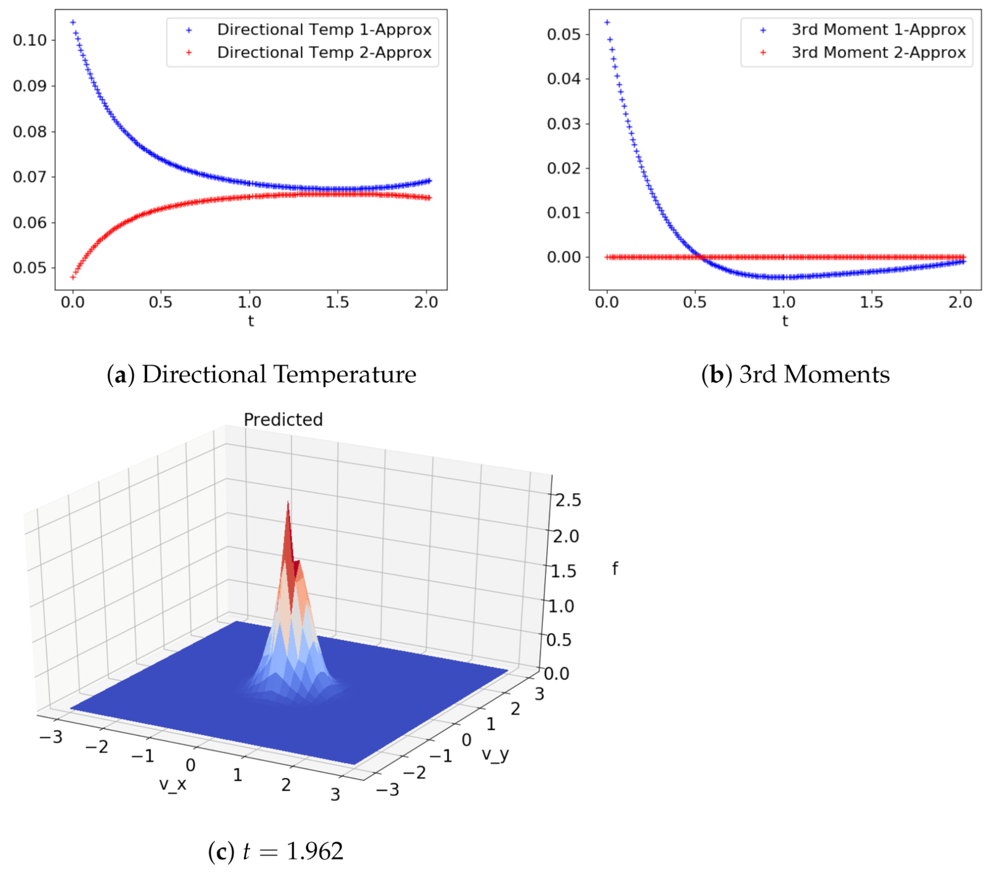
Solutions remained stable up until and beyond time values for which training data existed. Eventually though there was observed degradation and destabilization of the quality of predictions. Figure 9 demonstrates the long term behavior of the predicted solutions. Training data existed up until the dimensionless time $t=1.0$, and the simulation was run until $t=2.0$. The solution has clearly lost its shape by the end of that run; no longer having a nice Gaussian shape. In addition, the moments do not nicely converge to uniform values. The typical behavior was that the moments would tend towards the appropriate steady state early on, but would eventually begin to diverge. We propose that this behavior could be corrected by replacing the machine-learned model with an analytical method once the solution is close to steady state. This would ensure the appropriate long term behavior, and would still run much faster than using a direct discretization method for the full duration. Additionally, we are confident a more advanced architecture can be developed which achieves better accuracy and will likely still be faster than the true method. Even a model architecture that requires ten times the computational work of this simple model would still be tremendously time saving.

6. Conclusions

In an effort to advance the state-of-the-art in simulating complex flows, we have conducted investigations into the ability of machine learning to calculate the Boltzmann collision integral more quickly than traditional methods. Our experiments show that the machine-learned models are capable of finding low dimensional features that can encode the solutions with good accuracy. Consequently, predictions of the collision integral are able to be computed in much less time than is required for analytical methods. In the spatially homogeneous case, this approach shows greatly accelerated integration time. The resulting approximate solutions and key moments are generally similar to those of the true solutions. A key weakness exhibited by the method is the long term degradation of the solutions. An ideal numerical method will convergence to the correct steady state solution, however we have observed that the method presented here does not. Future work will involve improving accuracy even further by implementing more sophisticated machine learning methods. This will include investigation of different model architectures, and incorporating the enforcement of conservation laws into the model and the training process.