
The Extended Log-Logistic Distribution: Inference and Actuarial Applications


Abstract
1. Introduction
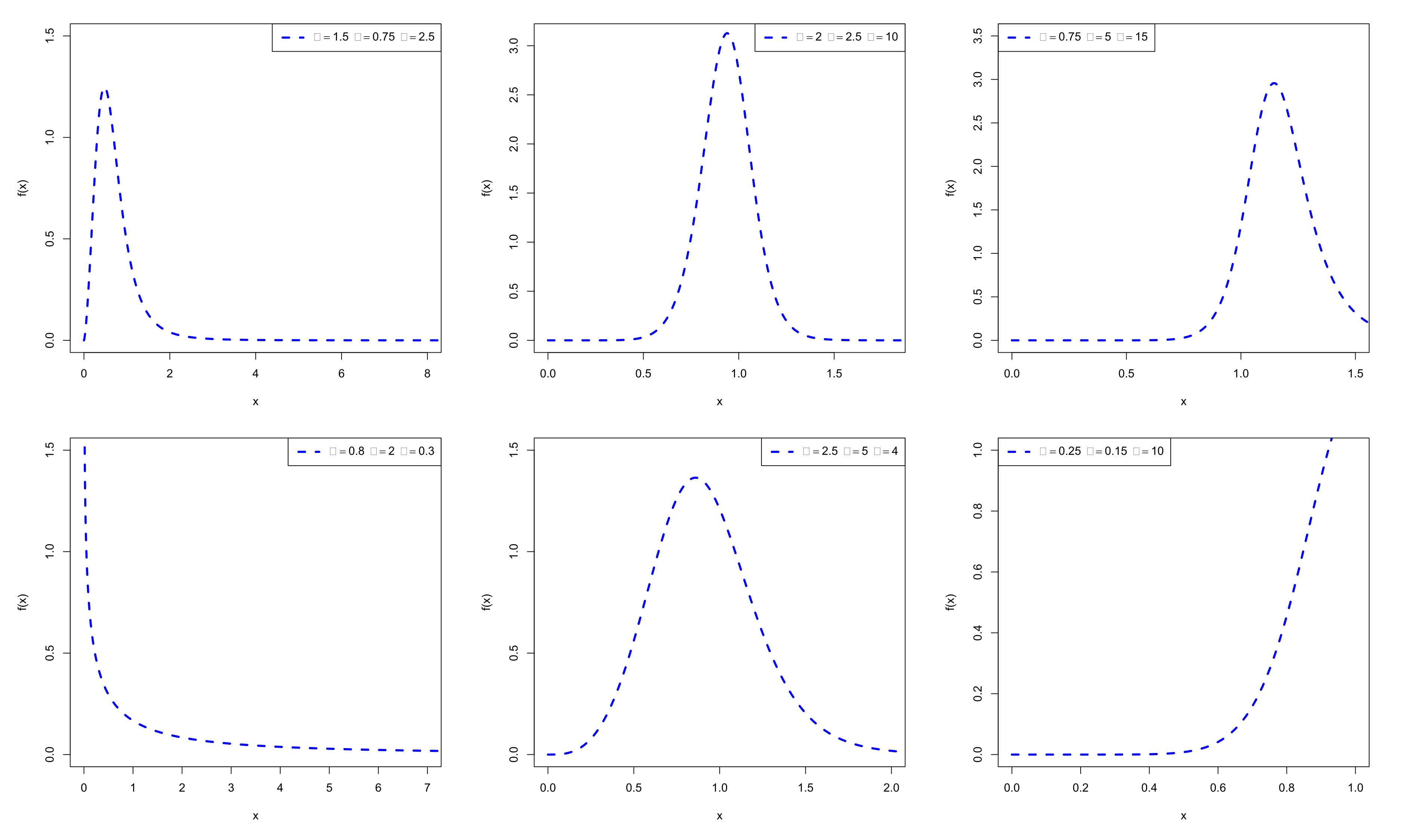
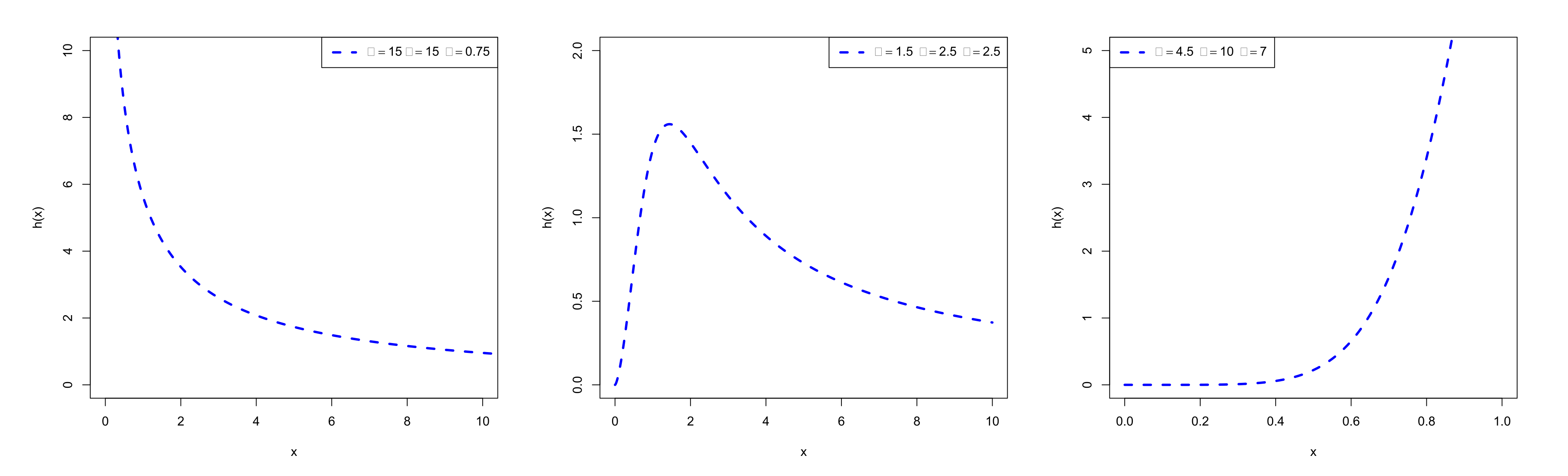
2. The Ex-LL Distribution
3. Mathematical Properties
3.1. Mode and Quantile Function
3.2. Moments and Moment Generating Function
3.3. Mean Residual Life, Mean Inactivity Time and Inequality Curves
3.4. Some Entropies
3.5. Order Statistics
4. Estimation Methods
4.1. Maximum Likelihood Estimation
4.2. Least-Squares and Weighted Least-Squares Estimation
4.3. Anderson—Darling Estimation
4.4. Cramér—Von Mises Estimation
5. Numerical Simulations for the Estimation Methods
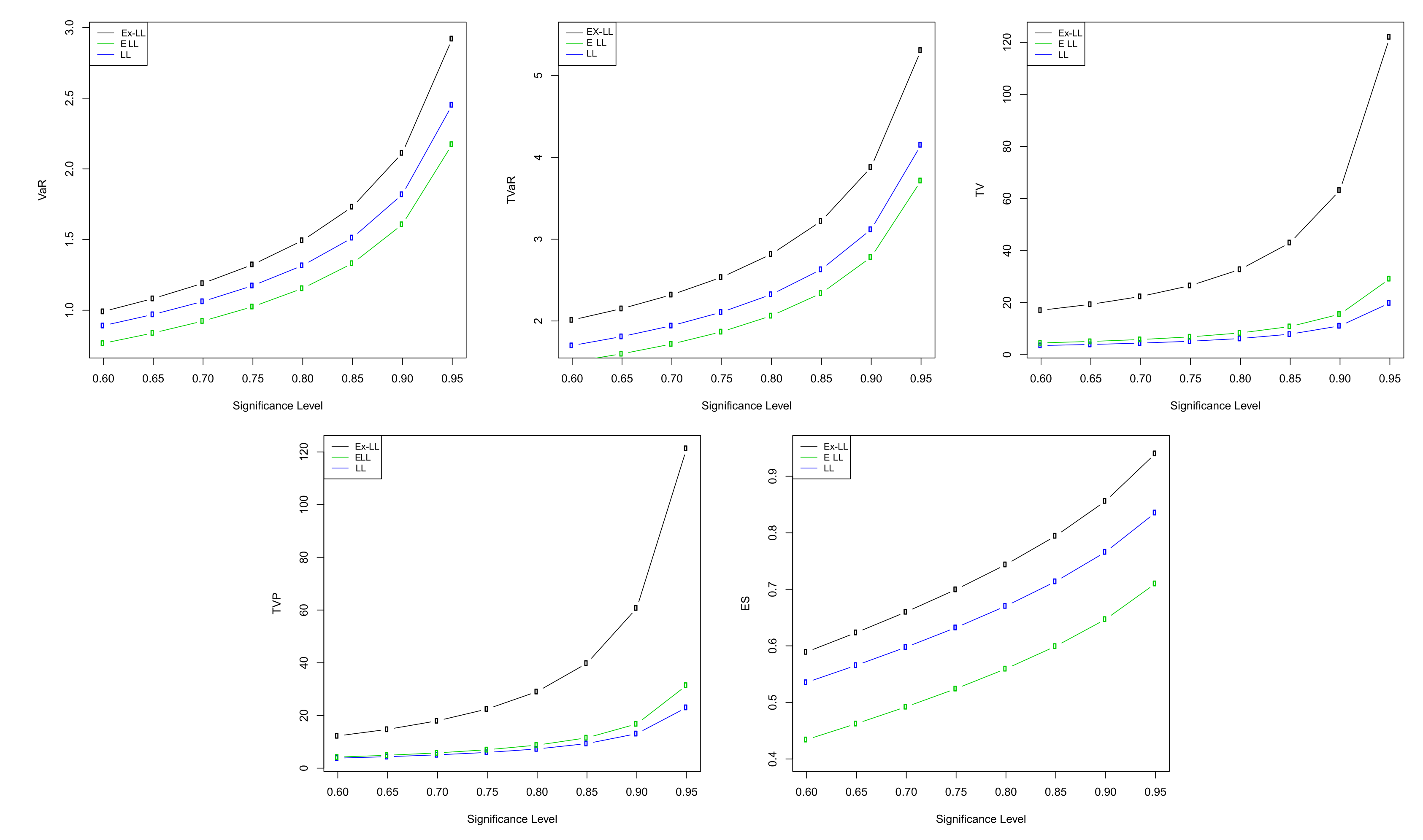
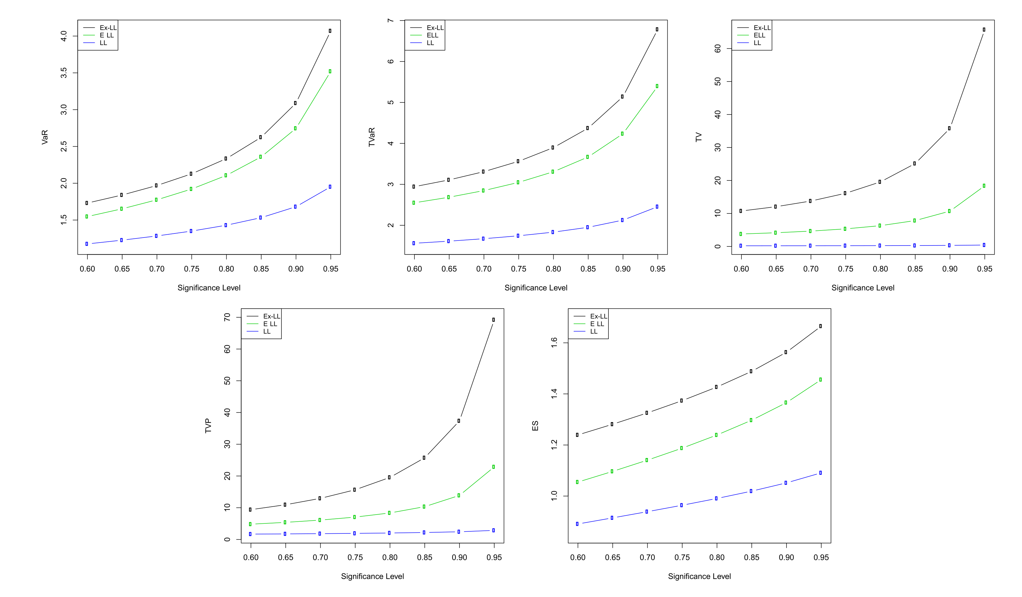
6. Actuarial Measures
6.1. VaR Measure
6.2. TVaR and TV Measures
6.3. TVP and ES Measures
6.4. Numerical Computations for Actuarial Measures
7. Modeling Real Data from the Engineering and Insurance Fields
8. Conclusions
Author Contributions
Funding
Acknowledgments
Conflicts of Interest
References
- Cooray, K.; Ananda, M.M.A. Modeling actuarial data with a composite lognormal-Pareto model. Scand. Actuar. J. 2005, 2005, 321–334. [Google Scholar] [CrossRef]
- Lane, M.N. Pricing risk transfer transactions 1. ASTIN Bull. J. IAA 2000, 30, 259–293. [Google Scholar] [CrossRef]
- Klugman, S.A.; Panjer, H.H.; Willmot, G.E. Loss Models: From Data to Decisions; John Wiley & Sons: Hoboken, NJ, USA, 2012; Volume 715. [Google Scholar]
- Ibragimov, R.; Prokhorov, A. Heavy Tails and Copulas: Topics in Dependence Modeling in Economics and Finance; World Scientific: Singapore, 2017. [Google Scholar]
- Punzo, A.; Mazza, A.; Maruotti, A. Fitting insurance and economic data with outliers: A flexible approach based on finite mixtures of contaminated gamma distributions. J. Appl. Stat. 2018, 45, 2563–2584. [Google Scholar] [CrossRef]
- Fisk, P.R. The graduation of income distributions. Econom. J. Econom. Soc. 1961, 29, 171–185. [Google Scholar] [CrossRef]
- Dagum, C. A model of income distribution and the conditions of existence of moments of finite order. Bull. Int. Stat. Inst. 1975, 46, 199–205. [Google Scholar]
- Shoukri, M.M.; Mian, I.U.H.; Tracy, D.S. Sampling properties of estimators of the log-logistic distribution with application to Canadian precipitation data. Can. J. Stat. 1988, 16, 223–236. [Google Scholar] [CrossRef]
- Arnold, B.C. Pareto Distributions Fairland; International Cooperative Publishing House: Silver Spring, MD, USA, 1983. [Google Scholar]
- Kleiber, C.; Kotz, S. Statistical Size Distributions in Economics and Actuarial Sciences; John Wiley & Sons: Hoboken, NJ, USA, 2003; Volume 470. [Google Scholar]
- De Santana, T.V.F.; Ortega, E.M.M.; Cordeiro, G.M.; Silva, G.O. The Kumaraswamy-log-logistic distribution. J. Stat. Theory Appl. 2012, 11, 265–291. [Google Scholar]
- Lemonte, A.J. The beta log-logistic distribution. Braz. J. Probab. Stat. 2014, 28, 313–332. [Google Scholar] [CrossRef]
- Gui, W. Marshall–Olkin extended log-logistic distribution and its application in minification processes. Appl. Math. Sci. 2013, 7, 3947–3961. [Google Scholar] [CrossRef]
- Tahir, M.H.; Mansoor, M.; Zubair, M.; Hamedani, G. McDonald log-logistic distribution with an application to breast cancer data. J. Stat. Theory Appl. 2014, 13, 65–82. [Google Scholar] [CrossRef]
- Hamedani, G. The Zografos-Balakrishnan log-logistic distribution: Properties and applications. J. Stat. Theory Appl. 2013, 12, 225–244. [Google Scholar]
- Cordeiro, G.M.; Afify, A.Z.; Ortega, E.M.; Suzuki, A.K.; Mead, M.E. The odd Lomax generator of distributions: Properties, estimation and applications. J. Comput. Appl. Math. 2019, 347, 222–237. [Google Scholar] [CrossRef]
- Zhao, W.; Khosa, S.K.; Ahmad, Z.; Aslam, M.; Afify, A.Z. Type-I heavy tailed family with applications in medicine, engineering and insurance. PLoS ONE 2020, 15, e0237462. [Google Scholar]
- Lorenz, M.O. Methods of measuring the concentration of wealth. Publ. Am. Stat. Assoc. 1905, 9, 209–219. [Google Scholar] [CrossRef]
- Bonferroni, C.E. Elementi di Statistica Generale; Seeber: Firenze, Italy, 1930. [Google Scholar]
- Arcagni, A.; Porro, F. The graphical representation of inequality. Rev. Colomb. De Estad. 2014, 37, 419–437. [Google Scholar] [CrossRef]
- Morales, D.; Pardo, L.; Vajda, I. Some new statistics for testing hypotheses in parametric models. J. Multivar. Anal. 1997, 62, 137–168. [Google Scholar] [CrossRef][Green Version]
- Kurths, J.; Voss, A.; Saparin, P.; Witt, A.; Kleiner, H.J.; Wessel, N. Quantitative analysis of heart rate variability. Chaos Interdiscip. J. Nonlinear Sci. 1995, 5, 88–94. [Google Scholar] [CrossRef]
- Song, K.S. Rényi information, loglikelihood and an intrinsic distribution measure. J. Stat. Plan. Inference 2001, 93, 51–69. [Google Scholar] [CrossRef]
- Galambos, J. The Asymptotic Theory of Extreme Order Statistics; R.E. Krieger Pub. Co.: Malabar, FL, USA, 1987. [Google Scholar]
- Artzner, P. Application of coherent risk measures to capital requirements in insurance. N. Am. Actuar. J. 1999, 3, 11–25. [Google Scholar] [CrossRef]
- Landsman, Z. On the tail mean—variance optimal portfolio selection. Insur. Math. Econ. 2010, 46, 547–553. [Google Scholar] [CrossRef]
- Kundu, D.; Raqab, M.Z. Estimation of R = P(Y < X) for three parameter Weibull distribution. Stat. Probab. Lett. 2009, 79, 1839–1846. [Google Scholar]
- Afify, A.; Cordeiro, G.; Butt, N.; Ortega, E.; Suzuki, A. A new lifetime model with variable shapes for the hazard rate. Braz. J. Probab. Stat. 2017, 31, 516–541. [Google Scholar] [CrossRef]
- Afify, A.; Mohamed, O. A new three-parameter exponential distribution with variable shapes for the hazard rate: Estimation and applications. Mathematics 2020, 8, 135. [Google Scholar] [CrossRef]
- Aldahlan, M.A. Alpha power transformed log-logistic distribution with application to breaking stress data. Adv. Math. Phys. 2020, 2020, 2193787. [Google Scholar] [CrossRef]
- Granzotto, D.C.T.; Louzada, F. The transmuted log-logistic distribution: Modeling, inference, and an application to a polled tabapua race time up to first calving data. Commun. Stat. Theory Methods 2015, 44, 3387–3402. [Google Scholar] [CrossRef]
- Adeyinka, F.S.; Olapade, A.K. On transmuted four parameters generalized log-logistic distribution. Int. J. Stat. Distrib. Appl. 2019, 5, 32–37. [Google Scholar]
- Almamy, J.A. Extended Poisson log-logistic distribution. Int. J. Stat. Probab. 2019, 8, 56–69. [Google Scholar] [CrossRef]
- Para, B.A.; Jan, T.R. Transmuted inverse log logistic model: Properties and application in medical sciences and engineering. Math. Theory Model. 2017, 7, 157–181. [Google Scholar]
- Abouelmagd, T.H.M.; Hamed, M.S.; Almamy, J.A.; Ali, M.M.; Yousof, H.M.; Korkmaz, M.C. Extended Weibull log-logistic distribution. J. Nonlinear Sci. Appl. 2019, 12, 523–534. [Google Scholar] [CrossRef][Green Version]


| Parameters | ||||
|---|---|---|---|---|
| 1.19852 | 0.05122 | 2.13181 | 15.34159 | |
| 1.11244 | 0.11314 | 2.34462 | 22.42470 | |
| 1.17775 | 0.43811 | 2.82183 | 49.06847 | |
| 0.74194 | 0.17386 | 2.82183 | 49.06840 | |
| 0.97440 | 0.009770 | 3.75522 | ||
| 0.94900 | 0.02378 | 0.10911 | 3.67376 | |
| 0.93367 | 0.05104 | 0.43449 | 4.10571 | |
| 0.41012 | 0.14478 | 3.58182 | 63.19551 | |
| 0.75546 | 0.49124 | 3.5818 | 63.19552 | |
| 0.86925 | 0.00610 | 3.66150 | ||
| 0.15610 | 0.01560 | 1.99387 | 11.18786 | |
| 0.82517 | 0.01221 | 3.39749 | ||
| 1.1 | 2.4 | 45.48282 | 2573.493 | |
| 0.84142 | 0.00184 | 4.31163 |
| Method | n | AVEs | |BIAS| | MSEs | MREs | ||||||||
|---|---|---|---|---|---|---|---|---|---|---|---|---|---|
| 20 | 0.45544 | 0.82322 | 0.42882 | 0.20092 | 0.57817 | 0.20749 | 0.05807 | 0.38638 | 0.43397 | 0.40184 | 0.77090 | 0.82998 | |
| 60 | 0.49767 | 0.85403 | 0.27882 | 0.13519 | 0.46744 | 0.05623 | 0.02582 | 0.28113 | 0.01014 | 0.27039 | 0.62326 | 0.22491 | |
| MLEs | 100 | 0.50470 | 0.84475 | 0.26361 | 0.10901 | 0.38399 | 0.03613 | 0.01709 | 0.20715 | 0.00250 | 0.21801 | 0.51198 | 0.14453 |
| 200 | 0.50599 | 0.82369 | 0.25548 | 0.08150 | 0.30228 | 0.02438 | 0.00984 | 0.14093 | 0.00102 | 0.16300 | 0.40304 | 0.09753 | |
| 400 | 0.50411 | 0.79550 | 0.25295 | 0.06234 | 0.22406 | 0.01847 | 0.00601 | 0.08300 | 0.00056 | 0.12469 | 0.29875 | 0.07387 | |
| 20 | 0.47006 | 0.85047 | 0.36550 | 0.17961 | 0.55206 | 0.15321 | 0.04672 | 0.36312 | 0.32044 | 0.35923 | 0.73609 | 0.61282 | |
| 60 | 0.49728 | 0.85796 | 0.27238 | 0.13283 | 0.45931 | 0.05222 | 0.02469 | 0.27227 | 0.00536 | 0.26565 | 0.61241 | 0.20888 | |
| ADEs | 100 | 0.49794 | 0.83269 | 0.26512 | 0.11280 | 0.39868 | 0.03958 | 0.01786 | 0.22022 | 0.00306 | 0.22561 | 0.53157 | 0.15832 |
| 200 | 0.50683 | 0.83278 | 0.25593 | 0.08694 | 0.32444 | 0.02628 | 0.01133 | 0.15956 | 0.00116 | 0.17388 | 0.43258 | 0.10510 | |
| 400 | 0.51133 | 0.81706 | 0.25103 | 0.06748 | 0.24631 | 0.01921 | 0.00692 | 0.09611 | 0.00059 | 0.13496 | 0.32841 | 0.07682 | |
| 20 | 0.43719 | 0.83250 | 0.45411 | 0.20364 | 0.59180 | 0.23453 | 0.05934 | 0.39988 | 0.36734 | 0.40729 | 0.78907 | 0.93813 | |
| 60 | 0.47816 | 0.84229 | 0.29655 | 0.14841 | 0.50060 | 0.07414 | 0.03061 | 0.30716 | 0.01561 | 0.29681 | 0.66747 | 0.29658 | |
| CVMEs | 100 | 0.49590 | 0.84021 | 0.26977 | 0.12305 | 0.43532 | 0.04692 | 0.02087 | 0.25272 | 0.00445 | 0.24611 | 0.58043 | 0.18766 |
| 200 | 0.49769 | 0.80971 | 0.26128 | 0.10032 | 0.35700 | 0.03228 | 0.01407 | 0.18118 | 0.00185 | 0.20063 | 0.47601 | 0.12913 | |
| 400 | 0.50719 | 0.80858 | 0.25299 | 0.07733 | 0.28006 | 0.02237 | 0.00881 | 0.12201 | 0.00081 | 0.15465 | 0.37341 | 0.08949 | |
| 20 | 0.45847 | 0.82578 | 0.37292 | 0.20637 | 0.58905 | 0.17174 | 0.05844 | 0.39551 | 0.16133 | 0.41274 | 0.78540 | 0.68696 | |
| 60 | 0.48678 | 0.81618 | 0.28039 | 0.15045 | 0.48006 | 0.06498 | 0.03125 | 0.29138 | 0.01055 | 0.30091 | 0.64008 | 0.25991 | |
| LSEs | 100 | 0.50286 | 0.84874 | 0.26454 | 0.12220 | 0.43261 | 0.04449 | 0.02082 | 0.24967 | 0.00403 | 0.24440 | 0.57681 | 0.17796 |
| 200 | 0.50544 | 0.82622 | 0.25790 | 0.09767 | 0.34795 | 0.03139 | 0.01383 | 0.17468 | 0.00174 | 0.19534 | 0.46394 | 0.12557 | |
| 400 | 0.50557 | 0.80299 | 0.25280 | 0.07308 | 0.26556 | 0.02106 | 0.00828 | 0.11398 | 0.00075 | 0.14616 | 0.35407 | 0.08425 | |
| 20 | 0.42128 | 0.62919 | 0.37346 | 0.16618 | 0.36769 | 0.16154 | 0.04217 | 0.17687 | 0.20431 | 0.33236 | 0.49026 | 0.64616 | |
| 60 | 0.46021 | 0.68579 | 0.28047 | 0.10123 | 0.30033 | 0.05367 | 0.01668 | 0.11734 | 0.00909 | 0.20246 | 0.40044 | 0.21467 | |
| WLSEs | 100 | 0.47383 | 0.69804 | 0.26572 | 0.08736 | 0.27135 | 0.03702 | 0.01195 | 0.09499 | 0.00276 | 0.17472 | 0.36180 | 0.14808 |
| 200 | 0.48150 | 0.71748 | 0.25940 | 0.06735 | 0.22310 | 0.02559 | 0.00691 | 0.06495 | 0.00118 | 0.13469 | 0.29747 | 0.10237 | |
| 400 | 0.48988 | 0.73140 | 0.25519 | 0.05457 | 0.18547 | 0.01790 | 0.00428 | 0.04574 | 0.00054 | 0.10915 | 0.24729 | 0.07159 | |
| Method | n | AVEs | |BIAS| | MSEs | MREs | ||||||||
|---|---|---|---|---|---|---|---|---|---|---|---|---|---|
| 20 | 1.41153 | 0.52791 | 0.92737 | 0.52999 | 0.37135 | 0.23962 | 0.37676 | 0.16123 | 0.13372 | 0.35333 | 0.74271 | 0.31950 | |
| 60 | 1.48145 | 0.55751 | 0.81153 | 0.40645 | 0.34424 | 0.11364 | 0.21149 | 0.14125 | 0.02864 | 0.27097 | 0.68848 | 0.15152 | |
| MLEs | 100 | 1.50103 | 0.56398 | 0.78553 | 0.35953 | 0.31680 | 0.07982 | 0.16758 | 0.12507 | 0.01260 | 0.23969 | 0.63360 | 0.10643 |
| 200 | 1.50431 | 0.54874 | 0.77072 | 0.29413 | 0.27135 | 0.05785 | 0.11529 | 0.09963 | 0.00596 | 0.19609 | 0.54270 | 0.07713 | |
| 400 | 1.54652 | 0.58012 | 0.75478 | 0.24613 | 0.23991 | 0.04102 | 0.08372 | 0.08260 | 0.00276 | 0.16409 | 0.47981 | 0.05469 | |
| 20 | 1.31110 | 0.47318 | 0.90698 | 0.51427 | 0.37389 | 0.23058 | 0.36618 | 0.16295 | 0.11341 | 0.34285 | 0.74778 | 0.30744 | |
| 60 | 1.44458 | 0.54431 | 0.80616 | 0.41158 | 0.34272 | 0.11176 | 0.22592 | 0.14116 | 0.02706 | 0.27439 | 0.68544 | 0.14901 | |
| ADEs | 100 | 1.46757 | 0.54777 | 0.78539 | 0.37295 | 0.32857 | 0.08549 | 0.17888 | 0.13098 | 0.01374 | 0.24864 | 0.65714 | 0.11399 |
| 200 | 1.49099 | 0.54753 | 0.76732 | 0.31129 | 0.28337 | 0.05973 | 0.12804 | 0.10596 | 0.00605 | 0.20752 | 0.56674 | 0.07964 | |
| 400 | 1.51391 | 0.55180 | 0.75876 | 0.25225 | 0.23914 | 0.04359 | 0.08940 | 0.08230 | 0.00308 | 0.16817 | 0.47827 | 0.05812 | |
| 20 | 1.27258 | 0.47091 | 0.97473 | 0.56918 | 0.39746 | 0.29462 | 0.44307 | 0.17760 | 0.19027 | 0.37945 | 0.79492 | 0.39282 | |
| 60 | 1.44240 | 0.55826 | 0.81707 | 0.44389 | 0.36743 | 0.12505 | 0.25899 | 0.15689 | 0.03341 | 0.29593 | 0.73487 | 0.16674 | |
| CVMEs | 100 | 1.45890 | 0.55626 | 0.80078 | 0.41612 | 0.35277 | 0.10053 | 0.22259 | 0.14669 | 0.02185 | 0.27741 | 0.70554 | 0.13404 |
| 200 | 1.47705 | 0.55032 | 0.77750 | 0.36031 | 0.31680 | 0.06889 | 0.16615 | 0.12463 | 0.00886 | 0.24021 | 0.63360 | 0.09186 | |
| 400 | 1.49539 | 0.54816 | 0.76766 | 0.30443 | 0.27381 | 0.05074 | 0.12364 | 0.10077 | 0.00463 | 0.20295 | 0.54763 | 0.06766 | |
| 20 | 1.25855 | 0.48920 | 0.90873 | 0.55036 | 0.40474 | 0.25849 | 0.42880 | 0.18298 | 0.14353 | 0.36691 | 0.80948 | 0.34465 | |
| 60 | 1.40272 | 0.54430 | 0.81088 | 0.45438 | 0.37463 | 0.13135 | 0.27403 | 0.16106 | 0.03822 | 0.30292 | 0.74925 | 0.17513 | |
| LSEs | 100 | 1.42517 | 0.53875 | 0.79324 | 0.41560 | 0.35221 | 0.09948 | 0.22450 | 0.14637 | 0.02011 | 0.27707 | 0.70442 | 0.13265 |
| 200 | 1.46760 | 0.55255 | 0.77457 | 0.36010 | 0.31955 | 0.07163 | 0.16870 | 0.12682 | 0.00979 | 0.24007 | 0.63909 | 0.09550 | |
| 400 | 1.50127 | 0.55580 | 0.76257 | 0.30360 | 0.27733 | 0.04843 | 0.12120 | 0.10284 | 0.00414 | 0.20240 | 0.55466 | 0.06457 | |
| 20 | 1.28169 | 0.48653 | 0.88215 | 0.54249 | 0.39246 | 0.22283 | 0.40396 | 0.17376 | 0.11742 | 0.36166 | 0.78492 | 0.29711 | |
| 60 | 1.37571 | 0.50967 | 0.80492 | 0.43880 | 0.35596 | 0.11527 | 0.25421 | 0.14886 | 0.02946 | 0.29254 | 0.71192 | 0.15369 | |
| WLSEs | 100 | 1.46830 | 0.55319 | 0.77985 | 0.37477 | 0.32993 | 0.08329 | 0.18007 | 0.13256 | 0.01314 | 0.24985 | 0.65986 | 0.11105 |
| 200 | 1.49321 | 0.55431 | 0.76960 | 0.31853 | 0.29148 | 0.06066 | 0.13340 | 0.10988 | 0.00663 | 0.21235 | 0.58295 | 0.08088 | |
| 400 | 1.51673 | 0.55744 | 0.75932 | 0.26604 | 0.24956 | 0.04460 | 0.09754 | 0.08778 | 0.00325 | 0.17736 | 0.49912 | 0.05946 | |
| Method | n | AVEs | |BIAS| | MSEs | MREs | ||||||||
|---|---|---|---|---|---|---|---|---|---|---|---|---|---|
| 20 | 1.85314 | 1.48999 | 0.31158 | 0.73785 | 1.02471 | 0.08048 | 0.74610 | 1.15826 | 0.01736 | 0.36893 | 0.68314 | 0.32193 | |
| 60 | 1.90010 | 1.51124 | 0.27375 | 0.57038 | 0.91181 | 0.03731 | 0.43609 | 0.95168 | 0.00294 | 0.28519 | 0.60787 | 0.14923 | |
| MLEs | 100 | 1.92990 | 1.52921 | 0.26407 | 0.49315 | 0.84142 | 0.02720 | 0.32231 | 0.82352 | 0.00139 | 0.24658 | 0.56095 | 0.10879 |
| 200 | 2.00622 | 1.61720 | 0.25649 | 0.39765 | 0.72007 | 0.01727 | 0.21150 | 0.64493 | 0.00056 | 0.19883 | 0.48004 | 0.06909 | |
| 400 | 1.99447 | 1.56795 | 0.25460 | 0.33997 | 0.63142 | 0.01338 | 0.15306 | 0.51363 | 0.00030 | 0.16998 | 0.42095 | 0.05354 | |
| 20 | 1.72200 | 1.38696 | 0.29740 | 0.69804 | 1.02208 | 0.07323 | 0.70656 | 1.16539 | 0.01284 | 0.34902 | 0.68138 | 0.29294 | |
| 60 | 1.82869 | 1.44691 | 0.26858 | 0.56224 | 0.90890 | 0.03673 | 0.43659 | 0.94701 | 0.00280 | 0.28112 | 0.60594 | 0.14693 | |
| ADEs | 100 | 1.87063 | 1.45446 | 0.26288 | 0.50596 | 0.83793 | 0.02689 | 0.34733 | 0.82977 | 0.00141 | 0.25298 | 0.55862 | 0.10754 |
| 200 | 1.91945 | 1.49514 | 0.25741 | 0.42940 | 0.76274 | 0.01887 | 0.24265 | 0.69713 | 0.00063 | 0.21470 | 0.50850 | 0.07549 | |
| 400 | 1.95698 | 1.51378 | 0.25461 | 0.36280 | 0.65160 | 0.01326 | 0.17309 | 0.53883 | 0.00029 | 0.18140 | 0.43440 | 0.05304 | |
| 20 | 1.61667 | 1.27273 | 0.33639 | 0.81359 | 1.07118 | 0.10798 | 0.93812 | 1.29057 | 0.02862 | 0.40679 | 0.71412 | 0.43192 | |
| 60 | 1.78705 | 1.42209 | 0.28117 | 0.66140 | 1.00275 | 0.04712 | 0.59267 | 1.11512 | 0.00494 | 0.33070 | 0.66850 | 0.18848 | |
| CVMEs | 100 | 1.84697 | 1.46006 | 0.26819 | 0.57122 | 0.92311 | 0.03330 | 0.44008 | 0.96553 | 0.00237 | 0.28561 | 0.61541 | 0.13318 |
| 200 | 1.90668 | 1.51328 | 0.25988 | 0.48834 | 0.83406 | 0.02229 | 0.31400 | 0.81293 | 0.00094 | 0.24417 | 0.55604 | 0.08916 | |
| 400 | 1.93295 | 1.50741 | 0.25568 | 0.41197 | 0.73034 | 0.01572 | 0.22306 | 0.64811 | 0.00042 | 0.20599 | 0.48690 | 0.06286 | |
| 20 | 1.60099 | 1.32167 | 0.30946 | 0.76927 | 1.05451 | 0.09292 | 0.89264 | 1.25585 | 0.02188 | 0.38464 | 0.70301 | 0.37167 | |
| 60 | 1.78712 | 1.44056 | 0.27176 | 0.63829 | 0.99005 | 0.04311 | 0.55917 | 1.08696 | 0.00395 | 0.31915 | 0.66003 | 0.17243 | |
| LSEs | 100 | 1.83845 | 1.46657 | 0.26526 | 0.56044 | 0.92200 | 0.03126 | 0.42632 | 0.96197 | 0.00209 | 0.28022 | 0.61467 | 0.12505 |
| 200 | 1.87112 | 1.47376 | 0.26070 | 0.50198 | 0.84759 | 0.02308 | 0.33393 | 0.84025 | 0.00106 | 0.25099 | 0.56506 | 0.09230 | |
| 400 | 1.95600 | 1.54985 | 0.25485 | 0.41293 | 0.73354 | 0.01568 | 0.22228 | 0.65567 | 0.00043 | 0.20647 | 0.48902 | 0.06273 | |
| 20 | 1.62026 | 1.33165 | 0.30114 | 0.74460 | 1.06107 | 0.08086 | 0.82260 | 1.24371 | 0.01652 | 0.37230 | 0.70738 | 0.32345 | |
| 60 | 1.79192 | 1.41344 | 0.26863 | 0.60238 | 0.95058 | 0.03833 | 0.49514 | 1.01211 | 0.00307 | 0.30119 | 0.63372 | 0.15332 | |
| WLSEs | 100 | 1.86971 | 1.47801 | 0.26166 | 0.51454 | 0.86538 | 0.02850 | 0.36243 | 0.87311 | 0.00161 | 0.25727 | 0.57692 | 0.11401 |
| 200 | 1.93741 | 1.54087 | 0.25636 | 0.44350 | 0.78729 | 0.01905 | 0.25577 | 0.73088 | 0.00065 | 0.22175 | 0.52486 | 0.07619 | |
| 400 | 1.97894 | 1.56557 | 0.25381 | 0.35977 | 0.65664 | 0.01394 | 0.17146 | 0.55077 | 0.00033 | 0.17988 | 0.43776 | 0.05575 | |
| Method | n | AVEs | |BIAS| | MSEs | MREs | ||||||||
|---|---|---|---|---|---|---|---|---|---|---|---|---|---|
| 20 | 2.24560 | 2.64903 | 1.86198 | 0.77288 | 1.47282 | 0.46844 | 0.98041 | 2.89801 | 0.57068 | 0.30915 | 0.49094 | 0.31230 | |
| 60 | 2.25729 | 2.63147 | 1.61863 | 0.59737 | 1.36952 | 0.19191 | 0.56221 | 2.38995 | 0.07931 | 0.23895 | 0.45651 | 0.12794 | |
| MLEs | 100 | 2.33810 | 2.74689 | 1.57806 | 0.52603 | 1.26338 | 0.14449 | 0.41949 | 2.00936 | 0.04052 | 0.21041 | 0.42113 | 0.09632 |
| 200 | 2.42485 | 2.93535 | 1.53902 | 0.41483 | 1.08489 | 0.09320 | 0.25331 | 1.46911 | 0.01563 | 0.16593 | 0.36163 | 0.06213 | |
| 400 | 2.42592 | 2.89977 | 1.52715 | 0.36439 | 0.97387 | 0.07037 | 0.18736 | 1.20044 | 0.00867 | 0.14576 | 0.32462 | 0.04691 | |
| 20 | 1.96643 | 2.22208 | 1.81809 | 0.86504 | 1.67317 | 0.46106 | 1.17772 | 3.60422 | 0.53668 | 0.34601 | 0.55772 | 0.30737 | |
| 60 | 2.15967 | 2.49301 | 1.63461 | 0.64438 | 1.45352 | 0.22280 | 0.67819 | 2.70468 | 0.10543 | 0.25775 | 0.48451 | 0.14853 | |
| ADEs | 100 | 2.23278 | 2.60175 | 1.58387 | 0.56446 | 1.33984 | 0.15538 | 0.51867 | 2.32278 | 0.04837 | 0.22578 | 0.44661 | 0.10358 |
| 200 | 2.31263 | 2.72185 | 1.54640 | 0.47481 | 1.18999 | 0.10990 | 0.35107 | 1.82351 | 0.02218 | 0.18992 | 0.39666 | 0.07327 | |
| 400 | 2.36909 | 2.79513 | 1.52576 | 0.39547 | 1.03967 | 0.07402 | 0.23015 | 1.38118 | 0.00967 | 0.15819 | 0.34656 | 0.04935 | |
| 20 | 1.91910 | 2.21165 | 2.01548 | 0.93924 | 1.62648 | 0.62234 | 1.44421 | 3.73631 | 0.95156 | 0.37570 | 0.54216 | 0.41489 | |
| 60 | 2.05856 | 2.35779 | 1.69367 | 0.72607 | 1.54565 | 0.27475 | 0.88149 | 3.14012 | 0.19211 | 0.29043 | 0.51522 | 0.18317 | |
| CVMEs | 100 | 2.14048 | 2.44608 | 1.62859 | 0.66368 | 1.48803 | 0.20009 | 0.70178 | 2.82250 | 0.08101 | 0.26547 | 0.49601 | 0.13339 |
| 200 | 2.27589 | 2.66818 | 1.56418 | 0.53037 | 1.27897 | 0.12895 | 0.44065 | 2.09930 | 0.03015 | 0.21215 | 0.42632 | 0.08596 | |
| 400 | 2.35226 | 2.79380 | 1.53631 | 0.44741 | 1.14970 | 0.08734 | 0.29189 | 1.64528 | 0.01335 | 0.17896 | 0.38323 | 0.05823 | |
| 20 | 1.85172 | 2.18912 | 1.86952 | 0.91448 | 1.60553 | 0.56718 | 1.42335 | 3.73097 | 0.78003 | 0.36579 | 0.53518 | 0.37812 | |
| 60 | 2.06210 | 2.40349 | 1.64521 | 0.72344 | 1.52299 | 0.26579 | 0.88558 | 3.08153 | 0.15334 | 0.28938 | 0.50766 | 0.17719 | |
| LSEs | 100 | 2.15266 | 2.49861 | 1.59454 | 0.63051 | 1.45032 | 0.18940 | 0.64817 | 2.69959 | 0.08013 | 0.25221 | 0.48344 | 0.12627 |
| 200 | 2.21830 | 2.56388 | 1.56615 | 0.56182 | 1.33145 | 0.13133 | 0.49994 | 2.28895 | 0.03368 | 0.22473 | 0.44382 | 0.08755 | |
| 400 | 2.31187 | 2.70032 | 1.53389 | 0.45719 | 1.15281 | 0.08493 | 0.31498 | 1.70177 | 0.01303 | 0.18288 | 0.38427 | 0.05662 | |
| 20 | 1.87451 | 2.17124 | 1.84122 | 0.93047 | 1.74185 | 0.49880 | 1.37506 | 3.87423 | 0.68065 | 0.37219 | 0.58062 | 0.33253 | |
| 60 | 2.09905 | 2.38931 | 1.63869 | 0.69261 | 1.52041 | 0.23253 | 0.77223 | 2.96559 | 0.12164 | 0.27704 | 0.50680 | 0.15502 | |
| WLSEs | 100 | 2.19562 | 2.52031 | 1.57188 | 0.59081 | 1.38196 | 0.15574 | 0.54307 | 2.40593 | 0.04481 | 0.23633 | 0.46065 | 0.10383 |
| 200 | 2.28638 | 2.65047 | 1.55164 | 0.49905 | 1.24121 | 0.11369 | 0.37638 | 1.94273 | 0.02405 | 0.19962 | 0.41374 | 0.07579 | |
| 400 | 2.37214 | 2.79379 | 1.52799 | 0.39952 | 1.05013 | 0.07544 | 0.23121 | 1.39508 | 0.00997 | 0.15981 | 0.35004 | 0.05030 | |
| Method | n | AVEs | |BIAS| | MSEs | MREs | ||||||||
|---|---|---|---|---|---|---|---|---|---|---|---|---|---|
| 20 | 0.50243 | 2.24341 | 3.28224 | 0.13748 | 0.94306 | 0.67856 | 0.02881 | 1.02669 | 0.58293 | 0.27496 | 0.47153 | 0.22619 | |
| 60 | 0.48696 | 2.11286 | 3.21149 | 0.10820 | 0.78843 | 0.50011 | 0.01652 | 0.76828 | 0.36328 | 0.21640 | 0.39422 | 0.16670 | |
| MLEs | 100 | 0.49448 | 2.07243 | 3.14715 | 0.09661 | 0.68849 | 0.41255 | 0.01330 | 0.61490 | 0.26279 | 0.19322 | 0.34424 | 0.13752 |
| 200 | 0.49851 | 2.07641 | 3.07894 | 0.07651 | 0.57391 | 0.30177 | 0.00849 | 0.45547 | 0.14912 | 0.15302 | 0.28695 | 0.10059 | |
| 400 | 0.50212 | 2.07711 | 3.04037 | 0.05995 | 0.47700 | 0.21511 | 0.00547 | 0.33087 | 0.07603 | 0.11990 | 0.23850 | 0.07170 | |
| 20 | 0.44274 | 2.01193 | 4.20196 | 0.16895 | 1.00339 | 1.60789 | 0.04291 | 1.18999 | 15.31004 | 0.33791 | 0.50169 | 0.53596 | |
| 60 | 0.48139 | 2.05736 | 3.27801 | 0.11600 | 0.80984 | 0.60048 | 0.02003 | 0.80657 | 0.78694 | 0.23201 | 0.40492 | 0.20016 | |
| ADEs | 100 | 0.49631 | 2.11680 | 3.15742 | 0.09698 | 0.73466 | 0.43798 | 0.01399 | 0.67913 | 0.38749 | 0.19396 | 0.36733 | 0.14599 |
| 200 | 0.49408 | 2.06002 | 3.09391 | 0.07580 | 0.60346 | 0.30384 | 0.00860 | 0.49172 | 0.16549 | 0.15160 | 0.30173 | 0.10128 | |
| 400 | 0.50434 | 2.08353 | 3.03178 | 0.06162 | 0.47980 | 0.22724 | 0.00570 | 0.33226 | 0.08575 | 0.12324 | 0.23990 | 0.07575 | |
| 20 | 0.47191 | 2.15401 | 3.34405 | 0.14059 | 0.97436 | 0.73788 | 0.02910 | 1.09771 | 0.66518 | 0.28118 | 0.48718 | 0.24596 | |
| 60 | 0.48488 | 2.13509 | 3.24755 | 0.11422 | 0.83868 | 0.56069 | 0.01828 | 0.84367 | 0.42795 | 0.22844 | 0.41934 | 0.18690 | |
| CVMEs | 100 | 0.48909 | 2.07422 | 3.16734 | 0.10394 | 0.78330 | 0.44853 | 0.01536 | 0.75647 | 0.30584 | 0.20788 | 0.39165 | 0.14951 |
| 200 | 0.49244 | 2.07016 | 3.11885 | 0.08338 | 0.65596 | 0.34937 | 0.01004 | 0.56122 | 0.19839 | 0.16676 | 0.32798 | 0.11646 | |
| 400 | 0.50562 | 2.10875 | 3.03711 | 0.06724 | 0.51606 | 0.25395 | 0.00668 | 0.37635 | 0.10448 | 0.13447 | 0.25803 | 0.08465 | |
| 20 | 0.48450 | 2.00972 | 3.20069 | 0.15733 | 1.01402 | 0.72415 | 0.03516 | 1.18199 | 0.65321 | 0.31466 | 0.50701 | 0.24138 | |
| 60 | 0.48641 | 2.00471 | 3.15364 | 0.12065 | 0.86235 | 0.54057 | 0.02068 | 0.89473 | 0.40918 | 0.24130 | 0.43118 | 0.18019 | |
| LSEs | 100 | 0.49040 | 2.03666 | 3.13691 | 0.10653 | 0.76666 | 0.45869 | 0.01595 | 0.72757 | 0.31329 | 0.21305 | 0.38333 | 0.15290 |
| 200 | 0.49555 | 2.03812 | 3.09514 | 0.08997 | 0.67809 | 0.34966 | 0.01139 | 0.58659 | 0.19512 | 0.17994 | 0.33905 | 0.11655 | |
| 400 | 0.50241 | 2.07492 | 3.04581 | 0.07053 | 0.53769 | 0.26944 | 0.00729 | 0.40341 | 0.11977 | 0.14105 | 0.26884 | 0.08981 | |
| 20 | 0.48996 | 1.97273 | 3.14295 | 0.15384 | 0.97597 | 0.70515 | 0.03462 | 1.11621 | 0.62033 | 0.30768 | 0.48799 | 0.23505 | |
| 60 | 0.49369 | 2.08173 | 3.14092 | 0.11013 | 0.78946 | 0.49356 | 0.01750 | 0.77294 | 0.35424 | 0.22026 | 0.39473 | 0.16452 | |
| WLSEs | 100 | 0.49501 | 2.05356 | 3.09485 | 0.09771 | 0.71978 | 0.41366 | 0.01356 | 0.65721 | 0.25556 | 0.19543 | 0.35989 | 0.13789 |
| 200 | 0.49602 | 2.03650 | 3.07105 | 0.07612 | 0.59806 | 0.29513 | 0.00837 | 0.47520 | 0.14243 | 0.15224 | 0.29903 | 0.09838 | |
| 400 | 0.50016 | 2.05893 | 3.04193 | 0.06049 | 0.47467 | 0.22367 | 0.00550 | 0.32886 | 0.08310 | 0.12098 | 0.23734 | 0.07456 | |
| Method | n | AVEs | |BIAS| | MSEs | MREs | ||||||||
|---|---|---|---|---|---|---|---|---|---|---|---|---|---|
| 20 | 0.83492 | 0.46297 | 2.24933 | 0.33119 | 0.37160 | 0.49496 | 0.14717 | 0.21310 | 0.36254 | 0.44159 | 1.48642 | 0.24748 | |
| 60 | 0.81841 | 0.40549 | 2.08986 | 0.24451 | 0.28605 | 0.32478 | 0.08961 | 0.14744 | 0.16990 | 0.32602 | 1.14421 | 0.16239 | |
| MLEs | 100 | 0.79325 | 0.36502 | 2.09112 | 0.21510 | 0.24491 | 0.28637 | 0.07033 | 0.11362 | 0.13963 | 0.28680 | 0.97962 | 0.14318 |
| 200 | 0.78636 | 0.32651 | 2.02668 | 0.15142 | 0.17165 | 0.18665 | 0.03876 | 0.06234 | 0.05959 | 0.20189 | 0.68661 | 0.09333 | |
| 400 | 0.76520 | 0.28487 | 2.02040 | 0.10656 | 0.11451 | 0.13671 | 0.01870 | 0.02552 | 0.03135 | 0.14208 | 0.45803 | 0.06836 | |
| 20 | 0.79889 | 0.43582 | 2.21286 | 0.31913 | 0.36183 | 0.50847 | 0.13592 | 0.20087 | 0.37146 | 0.42550 | 1.44731 | 0.25424 | |
| 60 | 0.79511 | 0.38007 | 2.10999 | 0.24857 | 0.27758 | 0.33594 | 0.09053 | 0.13852 | 0.18240 | 0.33143 | 1.11032 | 0.16797 | |
| ADEs | 100 | 0.79254 | 0.36612 | 2.07709 | 0.21196 | 0.24546 | 0.27375 | 0.06934 | 0.11501 | 0.12517 | 0.28261 | 0.98184 | 0.13688 |
| 200 | 0.78689 | 0.32595 | 2.02369 | 0.15182 | 0.17020 | 0.18431 | 0.03880 | 0.06073 | 0.05613 | 0.20243 | 0.68080 | 0.09215 | |
| 400 | 0.76688 | 0.28961 | 2.01599 | 0.11201 | 0.12121 | 0.14362 | 0.02059 | 0.02891 | 0.03319 | 0.14935 | 0.48485 | 0.07181 | |
| 20 | 0.82472 | 0.46533 | 2.26876 | 0.33654 | 0.38787 | 0.54958 | 0.14941 | 0.22490 | 0.42798 | 0.44872 | 1.55148 | 0.27479 | |
| 60 | 0.80202 | 0.40289 | 2.15938 | 0.27591 | 0.31266 | 0.38080 | 0.10554 | 0.16672 | 0.23498 | 0.36788 | 1.25062 | 0.19040 | |
| CVMEs | 100 | 0.80891 | 0.39274 | 2.09950 | 0.25005 | 0.28103 | 0.31747 | 0.08981 | 0.13985 | 0.16916 | 0.33340 | 1.12413 | 0.15874 |
| 200 | 0.79265 | 0.35382 | 2.05850 | 0.19409 | 0.21992 | 0.24060 | 0.05996 | 0.09739 | 0.09882 | 0.25879 | 0.87967 | 0.12030 | |
| 400 | 0.77411 | 0.30589 | 2.02115 | 0.13685 | 0.14992 | 0.16024 | 0.02992 | 0.04506 | 0.04103 | 0.18246 | 0.59969 | 0.08012 | |
| 20 | 0.79370 | 0.45012 | 2.16879 | 0.33067 | 0.37739 | 0.53675 | 0.14176 | 0.21563 | 0.40326 | 0.44089 | 1.50957 | 0.26837 | |
| 60 | 0.78499 | 0.38649 | 2.12663 | 0.27131 | 0.30138 | 0.38899 | 0.10137 | 0.15467 | 0.23666 | 0.36174 | 1.20554 | 0.19449 | |
| LSEs | 100 | 0.80486 | 0.39098 | 2.06359 | 0.24347 | 0.27741 | 0.31188 | 0.08636 | 0.13776 | 0.15902 | 0.32463 | 1.10964 | 0.15594 |
| 200 | 0.78174 | 0.33450 | 2.04287 | 0.18178 | 0.19988 | 0.22408 | 0.05314 | 0.08086 | 0.08415 | 0.24237 | 0.79951 | 0.11204 | |
| 400 | 0.78216 | 0.31606 | 2.01207 | 0.13903 | 0.15462 | 0.16389 | 0.03244 | 0.05026 | 0.04381 | 0.18537 | 0.61848 | 0.08195 | |
| 20 | 0.81442 | 0.46710 | 2.16386 | 0.33118 | 0.38694 | 0.51276 | 0.14430 | 0.22623 | 0.37333 | 0.44158 | 1.54776 | 0.25638 | |
| 60 | 0.80606 | 0.40889 | 2.08138 | 0.26430 | 0.30403 | 0.35064 | 0.09941 | 0.15848 | 0.20094 | 0.35240 | 1.21612 | 0.17532 | |
| WLSEs | 100 | 0.79000 | 0.35923 | 2.06213 | 0.21368 | 0.24001 | 0.28231 | 0.06998 | 0.10946 | 0.13010 | 0.28491 | 0.96003 | 0.14115 |
| 200 | 0.77623 | 0.32028 | 2.03488 | 0.15935 | 0.17806 | 0.20080 | 0.04068 | 0.06383 | 0.06655 | 0.21247 | 0.71225 | 0.10040 | |
| 400 | 0.76726 | 0.28926 | 2.01469 | 0.10864 | 0.11795 | 0.13961 | 0.01983 | 0.02892 | 0.03080 | 0.14485 | 0.47179 | 0.06980 | |
| AVEs | |BIAS| | MSEs | MREs | ||||||||||
|---|---|---|---|---|---|---|---|---|---|---|---|---|---|
| 20 | 0.46153 | 2.71277 | 0.95455 | 0.18905 | 1.33791 | 0.30181 | 0.04932 | 2.08963 | 0.15880 | 0.37809 | 0.53517 | 0.40241 | |
| 60 | 0.48363 | 2.64010 | 0.83440 | 0.12721 | 1.09299 | 0.16535 | 0.02427 | 1.49659 | 0.05432 | 0.25441 | 0.43720 | 0.22047 | |
| MLEs | 100 | 0.50133 | 2.68608 | 0.78893 | 0.10527 | 0.94619 | 0.11357 | 0.01660 | 1.16592 | 0.02334 | 0.21054 | 0.37848 | 0.15143 |
| 200 | 0.50499 | 2.70207 | 0.77399 | 0.08325 | 0.76398 | 0.08087 | 0.01013 | 0.82362 | 0.01201 | 0.16650 | 0.30559 | 0.10782 | |
| 400 | 0.50172 | 2.61169 | 0.76254 | 0.05946 | 0.57668 | 0.05462 | 0.00544 | 0.51692 | 0.00494 | 0.11892 | 0.23067 | 0.07282 | |
| 20 | 0.47205 | 2.76543 | 0.89752 | 0.17182 | 1.29764 | 0.26027 | 0.04250 | 1.96457 | 0.11997 | 0.34365 | 0.51906 | 0.34702 | |
| 60 | 0.49022 | 2.69752 | 0.81884 | 0.12708 | 1.11096 | 0.15657 | 0.02315 | 1.51754 | 0.04735 | 0.25416 | 0.44438 | 0.20877 | |
| ADEs | 100 | 0.49542 | 2.64261 | 0.79174 | 0.10748 | 0.97352 | 0.11482 | 0.01683 | 1.23172 | 0.02410 | 0.21496 | 0.38941 | 0.15310 |
| 200 | 0.50214 | 2.63223 | 0.76715 | 0.08471 | 0.79713 | 0.08182 | 0.01075 | 0.87469 | 0.01163 | 0.16943 | 0.31885 | 0.10910 | |
| 400 | 0.50391 | 2.60425 | 0.75934 | 0.06225 | 0.57941 | 0.05607 | 0.00585 | 0.51021 | 0.00508 | 0.12451 | 0.23176 | 0.07475 | |
| 20 | 0.45366 | 2.78292 | 0.95677 | 0.18705 | 1.35660 | 0.30773 | 0.04764 | 2.11219 | 0.15895 | 0.37410 | 0.54264 | 0.41030 | |
| 60 | 0.48393 | 2.79942 | 0.84624 | 0.13555 | 1.14799 | 0.18161 | 0.02632 | 1.61091 | 0.06553 | 0.27109 | 0.45920 | 0.24214 | |
| CVMEs | 100 | 0.48905 | 2.67878 | 0.81234 | 0.11520 | 1.01129 | 0.13716 | 0.01938 | 1.30345 | 0.03667 | 0.23040 | 0.40451 | 0.18289 |
| 200 | 0.49558 | 2.64128 | 0.78536 | 0.09394 | 0.85106 | 0.09981 | 0.01302 | 1.00094 | 0.01855 | 0.18787 | 0.34043 | 0.13308 | |
| 400 | 0.50474 | 2.63547 | 0.76320 | 0.07443 | 0.68258 | 0.06820 | 0.00830 | 0.68628 | 0.00778 | 0.14887 | 0.27303 | 0.09093 | |
| 20 | 0.46485 | 2.48793 | 0.89969 | 0.20045 | 1.40815 | 0.29410 | 0.05378 | 2.29446 | 0.14425 | 0.40089 | 0.56326 | 0.39213 | |
| 60 | 0.47964 | 2.60632 | 0.83485 | 0.14323 | 1.17969 | 0.18224 | 0.02876 | 1.67940 | 0.06566 | 0.28646 | 0.47187 | 0.24298 | |
| LSEs | 100 | 0.48933 | 2.61250 | 0.80603 | 0.12078 | 1.04900 | 0.13704 | 0.02053 | 1.37201 | 0.03665 | 0.24157 | 0.41960 | 0.18272 |
| 200 | 0.50076 | 2.62396 | 0.77556 | 0.09639 | 0.85770 | 0.09788 | 0.01346 | 0.97896 | 0.01749 | 0.19278 | 0.34308 | 0.13050 | |
| 400 | 0.50605 | 2.63179 | 0.75787 | 0.07262 | 0.68215 | 0.06507 | 0.00786 | 0.68552 | 0.00676 | 0.14523 | 0.27286 | 0.08676 | |
| 20 | 0.48081 | 2.62103 | 0.87745 | 0.19272 | 1.35298 | 0.27448 | 0.05168 | 2.13699 | 0.13228 | 0.38545 | 0.54119 | 0.36598 | |
| 60 | 0.48762 | 2.61203 | 0.81217 | 0.12827 | 1.10342 | 0.15156 | 0.02411 | 1.51895 | 0.04482 | 0.25654 | 0.44137 | 0.20208 | |
| WLSEs | 100 | 0.50143 | 2.68694 | 0.78520 | 0.10823 | 0.99737 | 0.11820 | 0.01709 | 1.26456 | 0.02637 | 0.21646 | 0.39895 | 0.15760 |
| 200 | 0.50581 | 2.69735 | 0.76913 | 0.08709 | 0.82057 | 0.08384 | 0.01109 | 0.91942 | 0.01160 | 0.17419 | 0.32823 | 0.11178 | |
| 400 | 0.50639 | 2.60810 | 0.75496 | 0.06065 | 0.58635 | 0.05395 | 0.00571 | 0.52327 | 0.00462 | 0.12131 | 0.23454 | 0.07194 | |
| Method | n | AVEs | |BIAS| | MSEs | MREs | ||||||||
|---|---|---|---|---|---|---|---|---|---|---|---|---|---|
| 20 | 2.02056 | 0.87123 | 1.75268 | 0.75361 | 0.60040 | 0.37441 | 0.72176 | 0.40677 | 0.24670 | 0.37680 | 0.80053 | 0.24961 | |
| 60 | 2.04596 | 0.90606 | 1.58218 | 0.59371 | 0.55020 | 0.18982 | 0.45335 | 0.35824 | 0.06828 | 0.29685 | 0.73360 | 0.12655 | |
| MLEs | 100 | 2.03551 | 0.88457 | 1.56159 | 0.53118 | 0.50936 | 0.14718 | 0.36724 | 0.31873 | 0.04348 | 0.26559 | 0.67914 | 0.09812 |
| 200 | 2.03433 | 0.85937 | 1.53411 | 0.45860 | 0.45067 | 0.10724 | 0.27391 | 0.26548 | 0.02019 | 0.22930 | 0.60089 | 0.07150 | |
| 400 | 2.05591 | 0.86550 | 1.51165 | 0.36412 | 0.37504 | 0.07650 | 0.18431 | 0.20053 | 0.00972 | 0.18206 | 0.50006 | 0.05100 | |
| 20 | 1.59765 | 0.53685 | 1.76036 | 0.66074 | 0.43279 | 0.38211 | 0.66528 | 0.23666 | 0.25494 | 0.33037 | 0.57706 | 0.25474 | |
| 60 | 1.73484 | 0.61443 | 1.61213 | 0.48879 | 0.36901 | 0.20326 | 0.39090 | 0.17490 | 0.08294 | 0.24440 | 0.49202 | 0.13550 | |
| ADEs | 100 | 1.80913 | 0.65080 | 1.57623 | 0.40531 | 0.33106 | 0.15308 | 0.27071 | 0.14146 | 0.04761 | 0.20265 | 0.44141 | 0.10205 |
| 200 | 1.86591 | 0.67683 | 1.54618 | 0.33465 | 0.29295 | 0.10695 | 0.17778 | 0.11082 | 0.02107 | 0.16732 | 0.39059 | 0.07130 | |
| 400 | 1.90085 | 0.69379 | 1.53028 | 0.28738 | 0.26020 | 0.07660 | 0.12418 | 0.08740 | 0.01073 | 0.14369 | 0.34693 | 0.05107 | |
| 20 | 1.60021 | 0.53982 | 1.84033 | 0.71141 | 0.43441 | 0.45749 | 0.76888 | 0.24432 | 0.33633 | 0.35571 | 0.57922 | 0.30499 | |
| 60 | 1.70061 | 0.59676 | 1.69293 | 0.56319 | 0.39183 | 0.27727 | 0.51422 | 0.19922 | 0.15218 | 0.28160 | 0.52243 | 0.18485 | |
| CVMEs | 100 | 1.76260 | 0.62855 | 1.61511 | 0.47324 | 0.36525 | 0.19052 | 0.36568 | 0.17017 | 0.07308 | 0.23662 | 0.48700 | 0.12701 |
| 200 | 1.79483 | 0.64084 | 1.58012 | 0.41277 | 0.33641 | 0.13674 | 0.27498 | 0.14544 | 0.03813 | 0.20639 | 0.44855 | 0.09116 | |
| 400 | 1.87348 | 0.68178 | 1.53910 | 0.32180 | 0.28266 | 0.08595 | 0.16065 | 0.10293 | 0.01438 | 0.16090 | 0.37688 | 0.05730 | |
| 20 | 1.58241 | 0.58488 | 1.69564 | 0.65138 | 0.41516 | 0.37637 | 0.68332 | 0.22305 | 0.24430 | 0.32569 | 0.55354 | 0.25091 | |
| 60 | 1.68550 | 0.60271 | 1.63653 | 0.53091 | 0.38273 | 0.23533 | 0.47255 | 0.18963 | 0.11102 | 0.26546 | 0.51031 | 0.15689 | |
| LSEs | 100 | 1.74643 | 0.62611 | 1.59427 | 0.47012 | 0.36568 | 0.18290 | 0.36683 | 0.16959 | 0.06656 | 0.23506 | 0.48758 | 0.12193 |
| 200 | 1.80075 | 0.64544 | 1.56000 | 0.39626 | 0.32886 | 0.12646 | 0.25467 | 0.13800 | 0.03148 | 0.19813 | 0.43848 | 0.08431 | |
| 400 | 1.88573 | 0.69750 | 1.53286 | 0.32604 | 0.28731 | 0.08698 | 0.16230 | 0.10455 | 0.01368 | 0.16302 | 0.38308 | 0.05799 | |
| 20 | 1.61320 | 0.58453 | 1.69765 | 0.64398 | 0.41260 | 0.36127 | 0.66479 | 0.21989 | 0.23351 | 0.32199 | 0.55013 | 0.24085 | |
| 60 | 1.73319 | 0.61795 | 1.61011 | 0.48655 | 0.36708 | 0.20733 | 0.39413 | 0.17357 | 0.08445 | 0.24327 | 0.48944 | 0.13822 | |
| WLSEs | 100 | 1.75203 | 0.61316 | 1.59444 | 0.44046 | 0.34836 | 0.16668 | 0.31873 | 0.15808 | 0.05398 | 0.22023 | 0.46448 | 0.11112 |
| 200 | 1.86835 | 0.67969 | 1.55063 | 0.34866 | 0.30253 | 0.10877 | 0.18761 | 0.11574 | 0.02104 | 0.17433 | 0.40338 | 0.07251 | |
| 400 | 1.92492 | 0.71359 | 1.52427 | 0.27331 | 0.25280 | 0.07229 | 0.11114 | 0.08122 | 0.00918 | 0.13665 | 0.33707 | 0.04819 | |
| Distribution | Parameters | Significance Level | VaR | TVaR | TV | TVP | ES |
|---|---|---|---|---|---|---|---|
| Ex-LL | 0.60 | 0.99108 | 2.01266 | 17.07036 | 12.25487 | 0.58926 | |
| 0.65 | 1.08279 | 2.15221 | 19.34957 | 14.72942 | 0.62361 | ||
| 0.70 | 1.19084 | 2.32171 | 22.36834 | 17.97955 | 0.66015 | ||
| 0.75 | 1.32315 | 2.53515 | 26.56123 | 22.45607 | 0.69977 | ||
| 0.80 | 1.49396 | 2.81781 | 32.79004 | 29.04984 | 0.74382 | ||
| 0.85 | 1.73244 | 3.22189 | 43.04476 | 39.80993 | 0.79451 | ||
| 0.90 | 2.11268 | 3.88033 | 63.21386 | 60.77280 | 0.85620 | ||
| 0.95 | 2.92095 | 5.30891 | 122.11669 | 121.31977 | 0.94018 | ||
| LL | 0.60 | 0.89125 | 1.70053 | 3.51346 | 3.80861 | 0.53540 | |
| 0.65 | 0.97023 | 1.81064 | 3.91554 | 4.35574 | 0.56574 | ||
| 0.70 | 1.06244 | 1.94324 | 4.44114 | 5.05204 | 0.59783 | ||
| 0.75 | 1.17421 | 2.10862 | 5.15965 | 5.97836 | 0.63240 | ||
| 0.80 | 1.31676 | 2.32522 | 6.20622 | 7.29019 | 0.67052 | ||
| 0.85 | 1.51287 | 2.63068 | 7.88611 | 9.33387 | 0.71395 | ||
| 0.90 | 1.81955 | 3.11972 | 11.07641 | 13.08849 | 0.76609 | ||
| 0.95 | 2.45266 | 4.15248 | 19.87667 | 23.03531 | 0.83561 | ||
| ELL | 0.60 | 0.76627 | 1.49988 | 4.52012 | 4.21195 | 0.43416 | |
| 0.65 | 0.83911 | 1.59959 | 5.08234 | 4.90311 | 0.46245 | ||
| 0.70 | 0.92366 | 1.71949 | 5.82319 | 5.79572 | 0.49229 | ||
| 0.75 | 1.02554 | 1.86882 | 6.84576 | 7.00314 | 0.52433 | ||
| 0.80 | 1.15475 | 2.06421 | 8.35301 | 8.74662 | 0.55951 | ||
| 0.85 | 1.33160 | 2.33966 | 10.80959 | 11.52781 | 0.59941 | ||
| 0.90 | 1.60692 | 2.78093 | 15.57473 | 16.79819 | 0.64706 | ||
| 0.95 | 2.17369 | 3.71548 | 29.18379 | 31.44008 | 0.71019 |
| Distribution | Parameters | Significance Level | VaR | TVaR | TV | TVP | ES |
|---|---|---|---|---|---|---|---|
| Ex-LL | 0.60 | 1.73116 | 2.94389 | 10.75330 | 9.39587 | 1.23942 | |
| 0.65 | 1.84031 | 3.10954 | 12.06103 | 10.94921 | 1.28134 | ||
| 0.70 | 1.96950 | 3.31065 | 13.77559 | 12.95357 | 1.32574 | ||
| 0.75 | 2.12859 | 3.56358 | 16.12836 | 15.65985 | 1.37375 | ||
| 0.80 | 2.33518 | 3.89777 | 19.57230 | 19.55561 | 1.42707 | ||
| 0.85 | 2.62516 | 4.37342 | 25.13698 | 25.73985 | 1.48847 | ||
| 0.90 | 3.08890 | 5.14234 | 35.80597 | 37.36772 | 1.56331 | ||
| 0.95 | 4.07034 | 6.78324 | 65.71723 | 69.21461 | 1.66531 | ||
| LL | 0.60 | 1.17575 | 1.56193 | 0.20470 | 1.68475 | 0.89085 | |
| 0.65 | 1.22690 | 1.61351 | 0.21234 | 1.75153 | 0.91470 | ||
| 0.70 | 1.28405 | 1.67328 | 0.22233 | 1.82891 | 0.93900 | ||
| 0.75 | 1.35008 | 1.74470 | 0.23566 | 1.92145 | 0.96415 | ||
| 0.80 | 1.42987 | 1.83374 | 0.25417 | 2.03708 | 0.99067 | ||
| 0.85 | 1.53286 | 1.95205 | 0.28165 | 2.19146 | 1.01939 | ||
| 0.90 | 1.68128 | 2.12727 | 0.32773 | 2.42222 | 1.05173 | ||
| 0.95 | 1.95220 | 2.45547 | 0.42938 | 2.86338 | 1.09106 | ||
| ELL | 0.60 | 1.54762 | 2.55035 | 3.77461 | 4.81512 | 1.05488 | |
| 0.65 | 1.65298 | 2.68624 | 4.15888 | 5.38951 | 1.09674 | ||
| 0.70 | 1.77511 | 2.84855 | 4.65763 | 6.10890 | 1.14072 | ||
| 0.75 | 1.92191 | 3.04906 | 5.33340 | 7.04911 | 1.18774 | ||
| 0.80 | 2.10724 | 3.30870 | 6.30683 | 8.35416 | 1.23916 | ||
| 0.85 | 2.35894 | 3.66969 | 7.84720 | 10.33981 | 1.29719 | ||
| 0.90 | 2.74555 | 4.23665 | 10.71635 | 13.88136 | 1.36600 | ||
| 0.95 | 3.52044 | 5.39809 | 18.39376 | 22.87216 | 1.45596 |
| 1.312 | 1.314 | 1.479 | 1.552 | 1.700 | 1.803 | 1.861 | 1.865 | 1.944 | 1.958 |
| 1.966 | 1.997 | 2.006 | 2.021 | 2.027 | 2.055 | 2.063 | 2.098 | 2.140 | 2.179 |
| 2.224 | 2.240 | 2.253 | 2.270 | 2.272 | 2.274 | 2.301 | 2.301 | 2.359 | 2.382 |
| 2.426 | 2.434 | 2.435 | 2.382 | 2.478 | 2.554 | 2.514 | 2.511 | 2.490 | 2.535 |
| 2.566 | 2.570 | 2.586 | 2.629 | 2.800 | 2.773 | 2.770 | 2.809 | 3.585 | 2.818 |
| 2.642 | 2.726 | 2.697 | 2.684 | 2.648 | 2.633 | 3.128 | 3.090 | 3.096 | 3.233 |
| 2.821 | 2.880 | 2.848 | 2.818 | 3.067 | 2.821 | 2.954 | 2.809 | 3.585 | 3.084 |
| 3.012 | 2.880 | 2.848 | 3.433 |
| 21 | 40 | 23 | 5 | 63 | 171 | 92 | 44 | 140 | 343 |
| 318 | 129 | 123 | 448 | 361 | 169 | 151 | 479 | 381 | 166 |
| 245 | 970 | 719 | 304 | 266 | 859 | 504 | 162 | 260 | 578 |
| 312 | 96 |
| Model | AD | CM | KS | KS-p-Value | Estimates (SEs) |
|---|---|---|---|---|---|
| Ex-LL | 0.18708 | 0.02454 | 0.05307 | 0.98524 | |
| LL | 0.56027 | 0.06756 | 0.05931 | 0.95704 | |
| APLL | 0.24447 | 0.03337 | 0.05432 | 0.98112 | |
| TLL | 0.28121 | 0.03938 | 0.05808 | 0.96415 | |
| GLL | 28.2565 | 6.1181 | 0.52316 | 0.0000 | |
| MOLL | 0.56027 | 0.06756 | 0.05931 | 0.95704 | |
| PBXLL | 1.10682 | 0.17631 | 0.09159 | 0.56396 | |
| TILL | 29.9400 | 6.55966 | 0.51579 | 0.0000 | |
| ILL | 54.7458 | 11.5014 | 0.66589 | 0.0000 | |
| WGLL | 0.21443 | 0.02648 | 0.05962 | 0.95509 | |
| Model | AD | CM | KS | KS-p-Value | Estimates (SEs) |
|---|---|---|---|---|---|
| Ex-LL | 0.14686 | 0.02332 | 0.07721 | 0.99108 | |
| LL | 0.43828 | 0.04824 | 0.08713 | 0.96832 | |
| APLL | 0.43812 | 0.04816 | 0.08704 | 0.96861 | |
| TLL | 0.43816 | 0.04818 | 0.08706 | 0.96853 | |
| GLL | 6.05879 | 1.23007 | 0.34740 | 0.00088 | |
| MOLL | 0.43828 | 0.04824 | 0.08712 | 0.96832 | |
| PBXLL | 0.84684 | 0.14436 | 0.14782 | 0.48651 | |
| TILL | 13.4133 | 2.93189 | 0.51187 | 0.00000 | |
| ILL | 24.0976 | 5.04201 | 0.67941 | ||
| WGLL | 0.30483 | 0.04463 | 0.08940 | 0.96016 | |
Publisher’s Note: MDPI stays neutral with regard to jurisdictional claims in published maps and institutional affiliations. |
© 2021 by the authors. Licensee MDPI, Basel, Switzerland. This article is an open access article distributed under the terms and conditions of the Creative Commons Attribution (CC BY) license (https://creativecommons.org/licenses/by/4.0/).
Share and Cite
Alfaer, N.M.; Gemeay, A.M.; Aljohani, H.M.; Afify, A.Z. The Extended Log-Logistic Distribution: Inference and Actuarial Applications. Mathematics 2021, 9, 1386. https://doi.org/10.3390/math9121386
Alfaer NM, Gemeay AM, Aljohani HM, Afify AZ. The Extended Log-Logistic Distribution: Inference and Actuarial Applications. Mathematics. 2021; 9(12):1386. https://doi.org/10.3390/math9121386
Chicago/Turabian StyleAlfaer, Nada M., Ahmed M. Gemeay, Hassan M. Aljohani, and Ahmed Z. Afify. 2021. "The Extended Log-Logistic Distribution: Inference and Actuarial Applications" Mathematics 9, no. 12: 1386. https://doi.org/10.3390/math9121386
APA StyleAlfaer, N. M., Gemeay, A. M., Aljohani, H. M., & Afify, A. Z. (2021). The Extended Log-Logistic Distribution: Inference and Actuarial Applications. Mathematics, 9(12), 1386. https://doi.org/10.3390/math9121386