An Online Generalized Multiscale Finite Element Method for Unsaturated Filtration Problem in Fractured Media

Abstract

In this paper, we present a multiscale model reduction technique for unsaturated filtration problem in fractured porous media using an Online Generalized Multiscale finite element method. The flow problem in unsaturated soils is described by the Richards equation. To approximate fractures we use the Discrete Fracture Model (DFM). Complex geometric features of the computational domain requires the construction of a fine grid that explicitly resolves the heterogeneities such as fractures. This approach leads to systems with a large number of unknowns, which require large computational costs. In order to develop a more efficient numerical scheme, we propose a model reduction procedure based on the Generalized Multiscale Finite element method (GMsFEM). The GMsFEM allows solving such problems on a very coarse grid using basis functions that can capture heterogeneities. In the GMsFEM, there are offline and online stages. In the offline stage, we construct snapshot spaces and solve local spectral problems to obtain multiscale basis functions. These spectral problems are defined in the snapshot space in each local domain. To improve the accuracy of the method, we add online basis functions in the online stage. The construction of the online basis functions is based on the local residuals. The use of online bases will allow us to get a significant improvement in the accuracy of the method. We present results with different number of offline and online multisacle basis functions. We compare all results with reference solution. Our results show that the proposed method is able to achieve high accuracy with a small computational cost.

1. Introduction

In this paper, we consider an unsaturated filtration problem in fractured heterogeneous media. For unsaturated filtration, we formulate a mathematical model that is based on the Richards’ equation [1,2,3,4,5]. Due to the high permeability of the fractures, these fractures have a significant effect on the flow processes and require a special approach in the construction of a mathematical model and computational algorithms. Such problems in fractured and heterogeneous media require very fine grids. Standard approaches use the finite element method to accurately model these processes [6,7,8]. Such approaches lead to large systems with large numbers of unknowns, and solving them is computationally expensive. Multiscale methods are designed to reduce the size of the system. A multiscale model reduction technique is based on the construction of multiscale basis functions to extract information in the micro-level. These basis functions are then used to obtain coarse scale equations.

Multiscale methods are widely used for simulation of problems in heterogeneous media, for example, multiscale finite element method (MsFEM) [9,10,11], multiscale finite volume method (MsFVM) [12,13,14], heterogeneous multiscale methods (HMM) [15,16], generalized multiscale finite element method (GMsFEM) [17,18,19], constraint energy minimizing generalized multiscale finite element method (CEM-GMsFEM) [20,21,22], mixed multiscale finite element method (Mixed MsFEM) [23,24,25]. For unsaturated filtration problem, the coarse grid approximation based on the MsFEM are constructed in [26,27,28], the authors present examples in heterogeneous media with high contrast. The upscaling method for the Richards equation are presented in [29]. In [30,31,32,33,34], the authors present a multiscale methods for filtration problem in fractured porous media. The effective algorithm of generalized multiscale finite element method (GMsFEM) for filtration problems in fractured heterogeneous porous media are developed in [30,35,36]. Recently in [37,38,39], the authors present a special type of multiscale basis functions based on constrained energy minimization problems and nonlocal multicontinuum (NLMC) method that uses this functions for problems in fractured porous media. Generalized multiscale finite element method (GMsFEM) for unsaturated filtration problems if fractured heterogeneous porous media are presented in our previous work [40]. An online generalized multiscale finite element method (Online GMsFEM) for filtration problem are presented in [41], and for Allen-Cahn problem are presented in [42].

In previous works the multiscale model reduction of Richards equation are presented, using offline multiscale basis functions [26,27,28,40].In this paper we use an online generalized multiscale finite element method. This method consists of offline and online stages. In the offline stage, we obtain multiscale basis functions by solving spectral problems in local domains. In particular, we will solve spectral problems on the snapshot space. The snapshot space helps us to take into account some complex properties of computational domain. Using snapshot space is justified for high-contrast heterogeneous domains, and for complex domains that contains fractures and channel. Using multiscale basis function we obtain an offline space on which we will solve our problem. In the online stage we solve our problem on the coarse grid using the offline space. For complex heterogenous problems, there is a need to enrich the approximation space using online basis functions. These online basis functions are computed adaptively in the online stage using local residuals. The aim is to reduce the error significantly by using a small number of these online basis functions. The motivation of the construction of online basis functions is the optimize the error reduction locally, and mathematical theories show that the online basis functions give fast convergence [41].

We will present numerical results for some two-dimensional examples. We consider two cases of fractured media. In the first case we take domains with simple network of fractures, and in the second case we test our method in domain with complex fracture network. We expect that, online basis functions will allow to us modeling unsaturated filtration process in all types of fracture geometry.

We organize the paper as follows. In Section 2, we present a mathematical model for unsaturated filtration problem in heterogeneous fractured media. In Section 3, we consider fine-scale approximation using a Discrete Fracture Model. Next in Section 4, we describe the construction of the coarse grid approximation and describe construction of the multiscale basis functions. In this Section, we present an offline multiscale basis functions and an online multiscale basis functions. We present numerical results in Section 5 for two-dimensional model problem. Finally, we present the Conclusion.

2. Problem Formulation

We use Richard’s equations to describe an unsaturated filtration process in fractured porous media. Let $\mathsf{\Omega }$ is the domain of the porous matrix. We consider lower dimensional fractures due to small thickness of the fractures compared to the domain sizes. We solve the following problem of the unsaturated filtration in fractured porous media

$$\begin{array}{cc}\hfill & \frac{\partial {\mathsf{\Theta }}_m}{\partial t}-\nabla ·(k_m(x,p_m)\nabla (p_m+z))+{\sigma }_{mf}(p_m-p_f)=f_m,x\in \mathsf{\Omega },\hfill \\ \hfill & \frac{\partial {\mathsf{\Theta }}_f}{\partial t}-\nabla ·(k_f(x,p_f)\nabla (p_f+z))-{\sigma }_{fm}(p_m-p_f)=f_f,x\in \gamma ,\hfill \end{array}$$

(1)

with following initial condition

$$p_m=p_f=p^0,$$

(2)

and boundary conditions

$$\begin{array}{cc}\hfill & p_m=p_f=g,x\in {\mathsf{\Gamma }}_D,\hfill \\ \hfill & \frac{\partial p_m}{\partial n}=\frac{\partial p_f}{\partial n}=0,x\in {\mathsf{\Gamma }}_N,\hfill \end{array}$$

(3)

where $\partial \mathsf{\Omega }={\mathsf{\Gamma }}_D\cup {\mathsf{\Gamma }}_N$, ${\mathsf{\Gamma }}_D$ is the top boundary of the computational domain and ${\mathsf{\Gamma }}_N$ denotes left, right, and bottom boundaries of the $\mathsf{\Omega }$. Here $p_m$ and $p_f$ are the pressure in matrix and fractures; $k_m$ and $k_f$ are the unsaturated hydraulic conductivity tensors for matrix and fractures; z is the influence of the gravity to the flow processes; ${\mathsf{\Theta }}_m$ and ${\mathsf{\Theta }}_f$ are the water content for matrix and fracture; and $f_m$ and $f_f$ denotes source and sink terms; ${\sigma }_{mf}$ and ${\sigma }_{fm}$ are transfer terms between matrix-fracture and fracture-matrix.

To define the physical properties of the domain $\mathsf{\Omega }$ we use Havercamp model [3]. Then, the non-linear coefficient $k_q(x,p_q)$ and the water content ${\mathsf{\Theta }}_q$ are determined as follows

$$\begin{array}{c}\hfill {\mathsf{\Theta }}_q(p_q)=\frac{{\alpha }_q({\mathsf{\Theta }}_{q,s}-{\mathsf{\Theta }}_{q,r})}{{\alpha }_q+{\left|p_q\right|}^{{\beta }_q}}+{\mathsf{\Theta }}_{q,r},k_q(x,p_q)=k_{q,s}(x)\frac{A_q}{A_q+{\left|p_q\right|}^{{\gamma }_q}},\end{array}$$

(4)

where $k_{q,s}(x)$ is the saturated hydraulic conductivity, ${\alpha }_q$${\beta }_q$, ${\gamma }_q$, $A_{\alpha }$, ${\mathsf{\Theta }}_{\alpha ,r}$, ${\mathsf{\Theta }}_{\alpha ,s}$ are the Haverkamp model coefficients and $q=m,f$.

3. Fine Grid Approximation

To perform numerical experiments, we solve a reference solution on a fine grid. We construct unstructured triangular fine grid that explicitly resolve fractures in the level of mesh. We construct an approximation on the fine grid by the finite element method and Discrete Fracture Model (DFM) for fracture networks. We have the weak formulation

$$\begin{array}{c}\hfill {\int }_{\mathsf{\Omega }}\frac{\partial {\mathsf{\Theta }}_m}{\partial t}{v}_{m}dx+{\int }_{\mathsf{\Omega }}\left(k_m\nabla p_m,\nabla v_m\right)dx-{\int }_{\mathsf{\Omega }}\frac{\partial k_m}{\partial z}{v}_{m}dx+\\ \hfill {\int }_{\mathsf{\Omega }}{\sigma }_{mf}(p_m-p_f)v_{m}dx={\int }_{\mathsf{\Omega }}{f}_m{v}_{m}dx,v_m\in {\widehat{V}}_m\\ \hfill {\int }_{\gamma }\frac{\partial {\mathsf{\Theta }}_f}{\partial t}{v}_{f}dx+{\int }_{\gamma }\left(k_f\nabla p_f,\nabla v_f\right)dx-{\int }_{\gamma }\frac{\partial k_f}{\partial z}{v}_{f}dx-\\ \hfill {\int }_{\gamma }{\sigma }_{fm}(p_m-p_f)v_{f}dx={\int }_{\gamma }{f}_f{v}_{f}dx,v_f\in {\widehat{V}}_f\end{array}$$

(5)

where $p=(p_m,p_f)\in V_m\times V_f$ and

$$V_m=\{v_m\in H^1(\mathsf{\Omega }):v=g,x\in {\mathsf{\Gamma }}_D\},V_f=\{v_f\in H^1(\gamma ):v=g,x\in {\mathsf{\Gamma }}_D\},$$

$${\widehat{V}}_m=\{v_m\in H^1(\mathsf{\Omega }):v=0,x\in {\mathsf{\Gamma }}_D\},{\widehat{V}}_f=\{v_f\in H^1(\gamma ):v=0,x\in {\mathsf{\Gamma }}_D\}.$$

For the approximation of the time derivative, we use the backward Euler method. To resolve non-linearity we use simplified approximation from the previous time step and obtain the following approximation on the fine grid

$$\begin{array}{c}\hfill {\int }_{\mathsf{\Omega }}{C}_m^n\frac{p_m^{n+1}-p_m^n}{\tau }{v}_{m}dx+{\int }_{\mathsf{\Omega }}\left(k_m^n\nabla p_m^{n+1},\nabla v_m\right)dx-{\int }_{\mathsf{\Omega }}\frac{\partial k_m^n}{\partial z}{v}_{m}dx+\\ \hfill {\int }_{\mathsf{\Omega }}{\sigma }_{mf}(p_m^{n+1}-p_f^{n+1})v_{m}dx={\int }_{\mathsf{\Omega }}{f}_m{v}_{m}dx,\\ \hfill {\int }_{\gamma }{C}_f^n\frac{p_f^{n+1}-p_f^n}{\tau }{v}_{f}dx+{\int }_{\gamma }\left(k_f^n\nabla p_f^{n+1},\nabla v_f\right)dx-{\int }_{\gamma }\frac{\partial k_f^n}{\partial z}{v}_{f}dx-\\ \hfill {\int }_{\gamma }{\sigma }_{fm}(p_m^{n+1}-p_f^{n+1})v_{f}dx={\int }_{\gamma }{f}_f{v}_{f}dx.\end{array}$$

(6)

where $\partial \mathsf{\Theta }(p_m)/\partial t=C(p_m)\partial p_m/\partial t$, $\partial \mathsf{\Theta }(p_f)/\partial t=C(p_f)\partial p_f/\partial t$, $C_m=d{\mathsf{\Theta }}_m/d{p}_m$, $C_f=d{\mathsf{\Theta }}_f/d{p}_f$, $C_m^n=C(p_m^n)$, $C_f^n=C(p_f^n)$, $k_m^n=k(x,p_m^n)$, $k_f^n=k(x,p_f^n)$ and

$$C_q(p_q)=-\frac{{\alpha }_q{\beta }_q({\mathsf{\Theta }}_{q,s}-{\mathsf{\Theta }}_{q,r}){\left|p_q\right|}^{{\beta }_q-2}{p}_q}{({\alpha }_q+|p_q{{|}^{{\beta }_q})}^2}.$$

We can write approximation, in the matrix form as

$$\frac{1}{\tau }\left(\begin{array}{cc}{S}_m^n& 0\\ 0& S_f^n\end{array}\right)\left(\begin{array}{c}{p}_m^{n+1}-p_m^n\\ p_f^{n+1}-p_f^n\end{array}\right)+\left(\begin{array}{cc}{A}_m^n+Q^n& -Q^n\\ -Q^n& A_f^n+Q^n\end{array}\right)\left(\begin{array}{c}{p}_m^{n+1}\\ p_f^{n+1}\end{array}\right)=\left(\begin{array}{c}{F}_m^n\\ F_f^n\end{array}\right)$$

(7)

To approximate lower dimensional fractures we use DFM approach. We assume that $p_m=p_f$ and using superposition principle [35,43] we eliminate $p_f$ from Equation (7) and obtain following system

$$S^n\frac{p^{n+1}-p^n}{\tau }+A^n{p}^{n+1}=F^n$$

(8)

where $S^n=S_m^n+S_f^n$, $A^n=A_m^n+A_f^n$ and $F^n=F_m^n+F_f^n$.

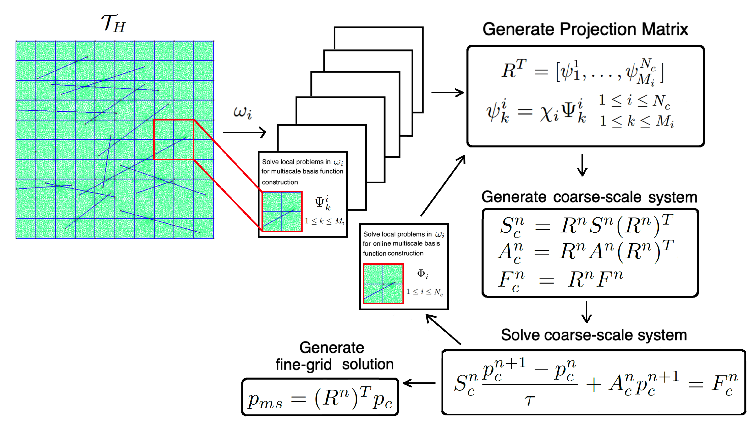
4. Coarse Grid Approximation

We construct a coarse grid approximation using an online generalized multiscale finite element method. Let ${\mathcal{T}}_H$ is the coarse grid and ${\omega }_i$ is the local domains, where $i=1,\dots ,N_c$ and $N_c$ is the number of coarse grid nodes. A local domain ${\omega }_i$ is obtained by the combining all the coarse cells around one vertex of the coarse grid.

The Online GMsFEM procedure consist of two parts (see Figure 1)

• Offline stage. In the offline stage we define an offline space by constructing an offline multiscale basis function;
• Online stage. In the online stage we construct the system on the offline space and enrich offline space by online multiscale basis functions.

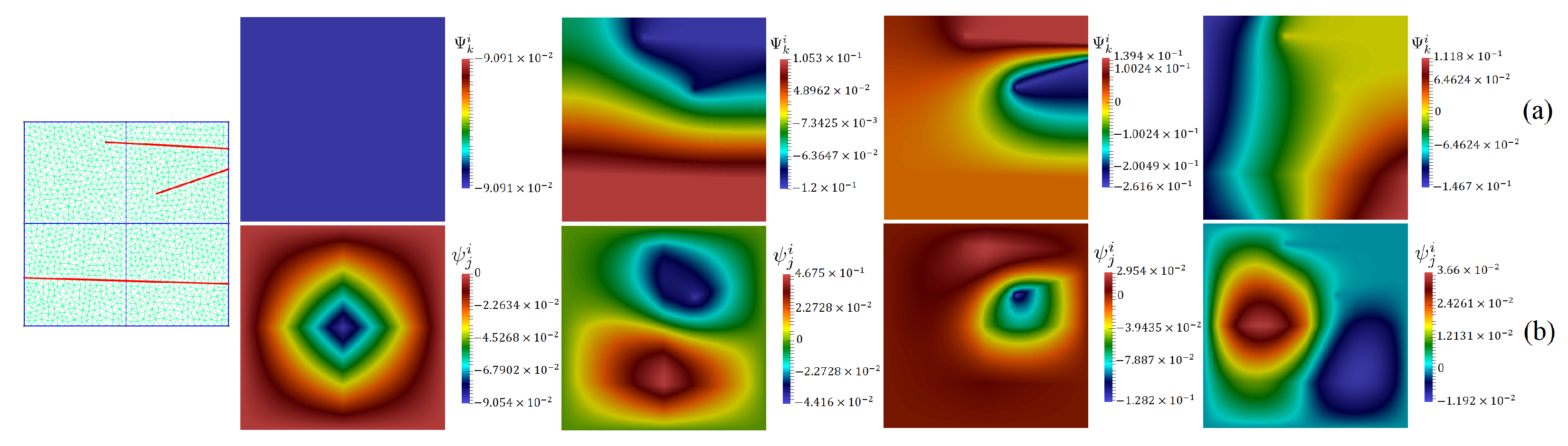
4.1. Offline Stage

We start from the constructing a snapshot space $V_{snap}^{{\omega }_i}$. The snapshot space are obtained by solving next local problems

$${\int }_{{\omega }_i}(k_{m,s}(x)\nabla {\varphi }_{m,j}^i,\nabla w_m^i)dx+{\int }_{\gamma }(k_{f,s}(x)\nabla {\varphi }_{f,j}^i,\nabla w_f^i)dx=0,$$

(9)

 with boundary condition ${\varphi }_{m,j}^i={\delta }_j,{\varphi }_{f,j}^i={\delta }_j$, where ${\delta }_j$ is the discrete delta function which takes the value 1 at the j-th fine grid node $x=x_j$ and zero elsewhere ($j=1,\dots ,J^i$, $J^i$ is number of fine grid nodes on boundary $\partial {\omega }_i$ ).

The main concept of constructing the snapshot space is that the snapshot vectors preserve some essential properties of the solution and provide a good approximation space. Snapshot space helps to better take into account heterogeneities with high contrast, as well as complex heterogeneities, such as channels and fractures. For the construction of the accurate approximation on the coarse grid for problems in fractured media, the number of dominant modes in spectral problem that corresponds to the very small eigenvalues should belong to the long fractures that cross the local domain boundaries. For the small separated fractures that do not cross the boundaries only one basis is sufficient for the approximation. When we skip construction of a snapshot space, a separate basis will be built for each small separate fracture. This approach will require more multiscale basis functions in each local domain ${\omega }_i$.

The snapshot space and the projection matrix on the snapshot space are defined as follows

$$V^{snap,i}=\mathrm{span}\{{\varphi }_1^i,\dots ,{\varphi }_{J_i}^i\},\mathrm{and}{R}_{snap,i}={({\varphi }_1^i,\dots ,{\varphi }_{J_i}^i)}^T.$$

On the snapshot space we solve the next local spectral problem in each ${\omega }_i$ to obtain an offline multiscale basis functions

$$\tilde{A}{\tilde{\mathsf{\Psi }}}_{snap,j}^i=\lambda \tilde{S}{\tilde{\mathsf{\Psi }}}_{snap,j}^i,$$

(10)

with

$$\tilde{A}=R_{snap,i}{A}^{{\omega }_i}{R}_{snap,i}^T,\tilde{S}=R_{snap,i}{S}^{{\omega }_i}{R}_{snap,i}^T,$$

where

$$\begin{array}{c}\hfill A^{{\omega }_i}=\left\{a_{ln}\right\},a_{ln}={\int }_{{\omega }_i}(k_{m,s}(x)\nabla {\psi }_{m,l},\nabla {\psi }_{m,n})dx+{\int }_{\gamma }(k_{f,s}(x)\nabla {\psi }_{f,l},\nabla {\psi }_{f,n})dx,\\ \hfill S^{{\omega }_i}=\left\{s_{ln}\right\},s_{ln}={\int }_{{\omega }_i}{k}_{m,s}(x){\psi }_{m,l}{\psi }_{m,n}dx+{\int }_{\gamma }{k}_{f,s}(x){\psi }_{f,l}{\psi }_{f,n}dx.\end{array}$$

(11)

We use solution of the spectral problem ${\mathsf{\Psi }}_j^i=R_{snap,i}{\tilde{\mathsf{\Psi }}}_{snap,j}^i$ in offline basis construction. We take only linear part $k_s(x)$ of coefficient $k(x,p)$ from (4). For basis construction we choose the smallest $M_i$ eigenvalues. We obtain an offline multiscale basis functions by multiplication on the linear partition of unity function ${\psi }_j^i={\chi }_i{\mathsf{\Psi }}_j^i$, where ${\chi }_i$ is the linear coarse grid nodal basis function that is equal to zero on the boundary of local domain ${\omega }_i$ and one at the coarse grid node i. An example of first 4 solution of spectral problem and first 4 offline multiscale basis functions are presented in Figure 2.

Now, we can define the offline space

$$V_{ms}=span({\psi }_1^1,\dots ,{\psi }_{M_1}^1,\dots ,{\psi }_1^{N_c},\dots ,{\psi }_{M_{N_c}}^{N_c}).$$

and projection matrix

$$R^T=({\psi }_1^1,\dots ,{\psi }_{M_1}^1,\dots ,{\psi }_1^{N_c},\dots ,{\psi }_{M_{N_c}}^{N_c}).$$

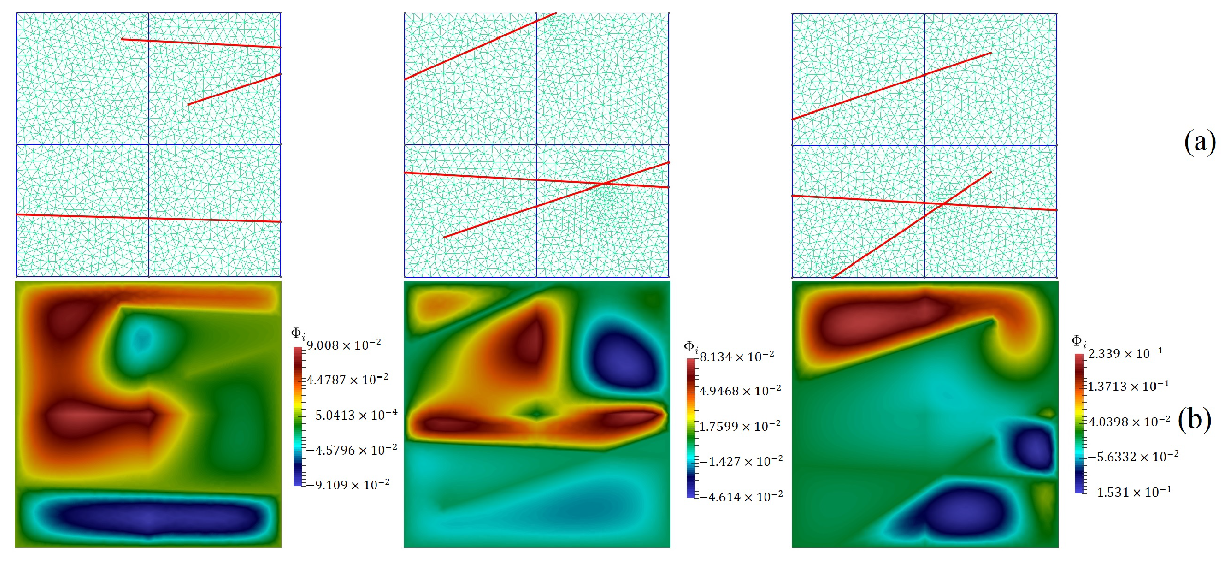
4.2. Online Stage

Since our problem is non-linear, we need to take into account the change in the coefficients over time. It is possible to consider ways of updating offline basis functions at certain time steps, but this approach has large computational costs. It would be much more profitable to add one basis to each local area, which minimizes the residual. This way is based on the online basis enrichment for GMsFEM based on the residual [41]. Presented procedure will allow us to significantly reduce the number of used offline multiscale basis functions and add local online multiscale basis functions to fast error reduction based on the local residual information. With fewer basis functions, we will be able to get better accuracy, since our bases will take into account the coefficient k changes over time.

In online GMsFEM, we update projection matrix $R^n$ by adding online residual based multiscale basis functions at n-th time step. Therefore, we solve next system on the coarse grid

$$S_c^n\frac{p_c^{n+1}-p_c^n}{\tau }+A_c^n{p}_c^{n+1}=F_c^n,$$

(12)

where coarse scale matrices and vectors are constructed using current projection matrix $R^n$

$$S_c^n=R^n{S}^n{(R^n)}^T,A_c^n=R^n{A}^n{(R^n)}^T,F_c^n=R^n{F}^n,p_{ms}^{n+1}={(R^n)}^T{p}_c^{n+1}.$$

Note that, when we use pre-constructed offline multiscale basis functions for given heterogeneity and fracture distribution in coarse scale system construction, we can use predefined projection matrix without updating it at n-th time step

$${(R^n)}^T=R^T=({\psi }_1^1,\dots ,{\psi }_{M_1}^1,\dots ,{\psi }_1^{N_c},\dots ,{\psi }_{M_{N_c}}^{N_c}).$$

In online GMsFEM, we set $R^n=R$ at first time step ($n=0$), then we construct and solve coarse scale system (12). Next, at time step $n=1,2,\dots$, we enrich multiscale space by residual based online multiscale basis functions. In order to enrich space, we solve system (12) with $R^n=R^{n-1}$, then we calculate online multiscale basis functions ${\vartheta }_1^i$ locally in ${\omega }_i$ using current residuals and update the projection matrix

$${(R^{1,n})}^T=({\psi }_1^1,\dots ,{\psi }_{M_1}^1,\dots ,{\psi }_1^{N_c},\dots ,{\psi }_{M_{N_c}}^{N_c},{\vartheta }_1^1,\dots ,{\vartheta }_1^{N_c}).$$

We can reiterate the process with residual calculation and add more online basis functions on the n-th time step

$${(R^n)}^T={(R^{L,n})}^T=({\psi }_1^1,\dots ,{\psi }_{M_1}^1,\dots ,{\psi }_1^{N_c},\dots ,{\psi }_{M_{N_c}}^{N_c},{\vartheta }_1^1,\dots ,{\vartheta }_{!}^{N_c}\dots ,{\vartheta }_L^1,\dots ,{\vartheta }_L^{N_c}),$$

where L is the number of online iterations. We can enrich multiscale space not for every time steps, for example, every 5-th or 10-th. Then, when we keep $R^n$ for the time steps where we do not want to update online basis functions. Next, we present construction of the online multiscale basis functions in local domain ${\omega }_i$ in details.

Construction of the local residual based online multiscale basis functions is based on the solution of the following local problem in ${\omega }_i$:

$$\begin{array}{c}\hfill a_{{\omega }_i}({\mathsf{\Phi }}_l^i,v)=r_{{\omega }_i}^l(v),l=1,\dots ,L,\end{array}$$

(13)

where

$$\begin{array}{cc}\hfill a_{{\omega }_i}({\mathsf{\Phi }}_l^i,v)& ={\int }_{{\omega }_i}{C}_m^n\frac{{\mathsf{\Phi }}_l^i}{\tau }vdx+{\int }_{{\omega }_i}\left(k_m^n\nabla {\mathsf{\Phi }}_l^i,\nabla v\right)dx+\hfill \\ \hfill & {\int }_{{\gamma }_i}{C}_f^n\frac{{\mathsf{\Phi }}_l^{f,i}}{\tau }{v}_{f}dx+{\int }_{{\gamma }_i}\left(k_f^n\nabla {\mathsf{\Phi }}_l^{f,i},\nabla v_f\right)dx,\hfill \\ \hfill r_{{\omega }_i}^l(v)& ={\int }_{{\omega }_i}\frac{\partial k_m^n}{\partial z}vdx+{\int }_{{\omega }_i}{f}_{m}vdx-{\int }_{{\omega }_i}{C}_m^n\frac{p_{m,ms}^{l,n+1}-p_{m,ms}^{l,n}}{\tau }vdx-\hfill \\ & {\int }_{{\omega }_i}\left(k_m^n\nabla p_{m,ms}^{l,n+1},\nabla v\right)dx+{\int }_{{\gamma }_i}\frac{\partial k_f^n}{\partial z}{v}_{f}dx+{\int }_{{\gamma }_i}{f}_f{v}_{f}dx-\hfill \\ \hfill & {\int }_{{\gamma }_i}{C}_f^n\frac{p_{f,ms}^{l,n+1}-p_{f,ms}^{l,n}}{\tau }{v}_{f}dx-{\int }_{{\gamma }_i}\left(k_f^n\nabla p_{f,ms}^{l,n+1},\nabla v_f\right)dx,\hfill \end{array}$$

(14)

with zero Dirichlet boundary condition ${\mathsf{\Phi }}_l^i=0,{\mathsf{\Phi }}_l^{f,i}=0$ on the $\partial {\omega }_i$. Finally, we obtain an online multiscale basis functions by multiplication on the linear partition of unity function ${\vartheta }_l^i={\chi }_i{\mathsf{\Phi }}_l^i$. We present solution of (13) and (14) for three different local domains in Figure 3 ($l=1$).

Using constructed online multiscale basis functions, we enrich the multiscale space by adding online basis functions ${\vartheta }_l^i$:

$$V_{ms}=span({\psi }_1^i,\dots ,{\psi }_{M_i}^i,{\vartheta }_l^1,\dots ,{\vartheta }_l^{N_c},i=1,\dots ,N_c,l=1,\dots ,L).$$

Here, we can add several online multiscale basis functions in local domain ${\omega }_i$ based on the current solution $p_{ms}^{l,n}$

$$S_c^{l,n}\frac{p_c^{l,n+1}-p_c^n}{\tau }+A_c^{l,n}{p}_c^{l,n+1}=F_c^{l,n},$$

(15)

where coarse scale matrices and vectors are constructed using current projection matrix $R^{l,n}$

$$S_c^{l,n}=R^{l,n}{S}^n{(R^{l,n})}^T,A_c^{l,n}=R^{l,n}{A}^n{(R^{l,n})}^T,F_c^{l,n}=R^{l,n}{F}^n,p_{ms}^{l,n+1}={(R^{l,n+!})}^T{p}_c^{l,n+1}.$$

with projection matrix

$$R^{l,n}={({\psi }_1^1,\dots ,{\psi }_{M_1}^1,\dots ,{\psi }_1^{N_c},\dots ,{\psi }_{M_{N_c}}^{N_c},{\vartheta }_1^1,\dots ,{\vartheta }_1^{N_c}\dots ,{\vartheta }_l^1,\dots ,{\vartheta }_l^{N_c})}^T,$$

where $l=1,\dots ,L$, $R^n=R^{L,n}$ and L is the number of the online iterations.

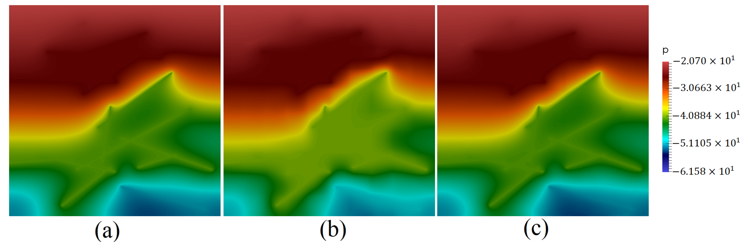
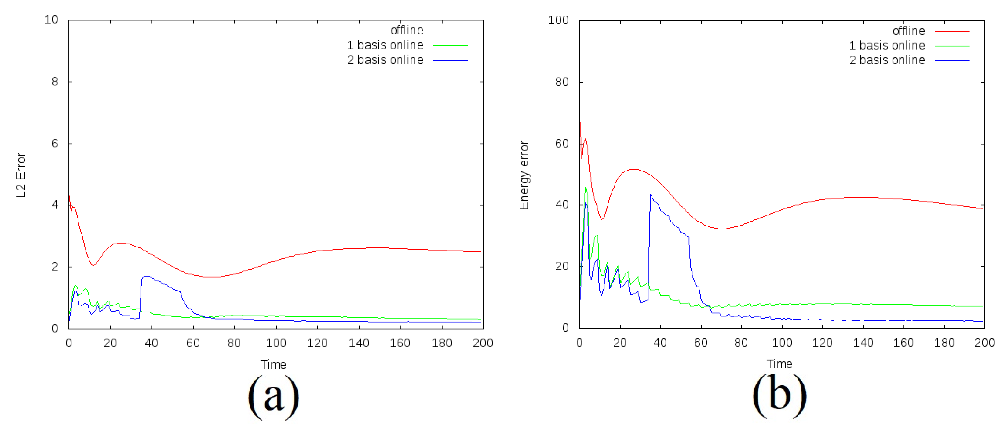
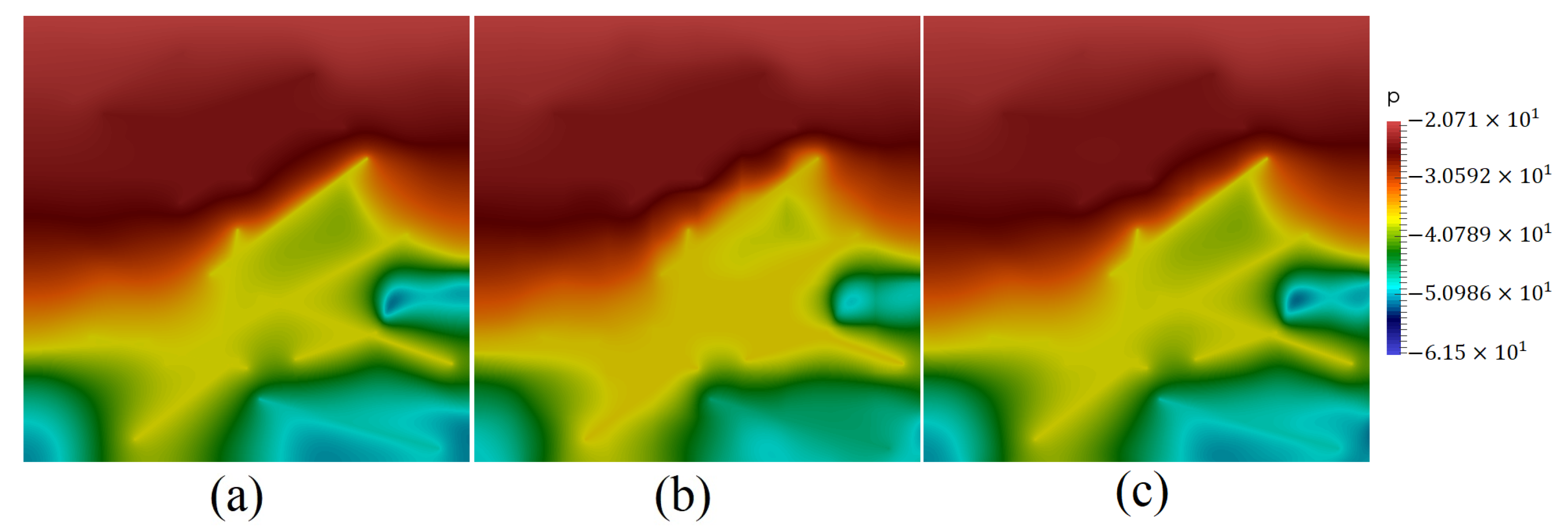
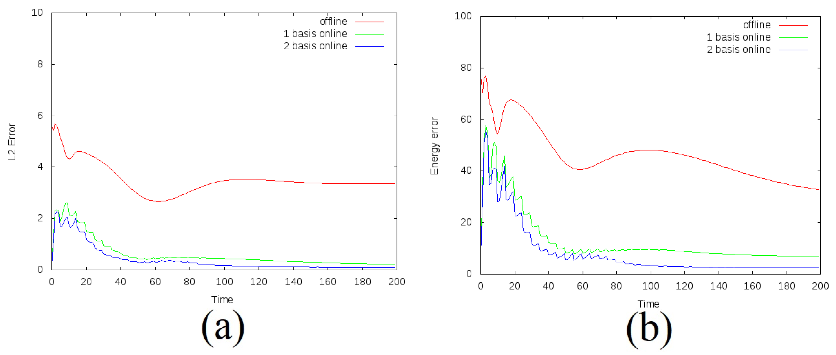
5. Numerical Results

We present numerical results for two-dimensional problem with in fractured heterogeneous media. We consider problems in two-dimensional domains with different fractures locations. In this work, we consider the following model problems:

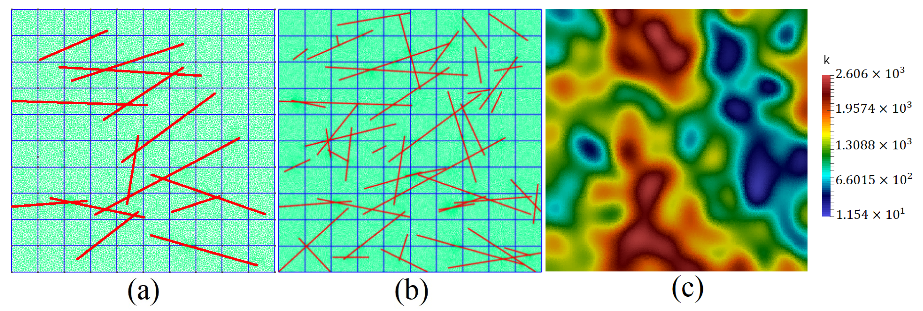
• Test 1. Computational domain with 14 fractures, $T_{max}=3\times {10}^{-3}$, $k_{m,s}=10$ and $k_{f,s}={10}^9$ (homogeneous porous matrix);
• Test 2. Computational domain with 14 fractures, $T_{max}=67\times {10}^{-7}$, $k_{m,s}=k_{m,s}(x)$ and $k_{f,s}={10}^9$ (heterogeneous porous matrix);
• Test 3. Computational domain with 50 fractures, $T_{max}=12\times {10}^{-7}$, $k_{m,s}=k_{m,s}(x)$ and $k_{f,s}={10}^9$ (heterogeneous porous matrix).

On the top boundary ${\mathsf{\Gamma }}_D$ we set Dirichlet boundary condition $p_1=-20.7$, as initial condition we take $p_0=-61.5$. The computational domains $\mathsf{\Omega }={[0,1]}^2$ and the domain properties $k_{m,s}(x)$ for Test 2 and Test 3 are presented in Figure 4. For domain with 14 fractures (Test 1,2), fine grid consist of 31,628 vertices and 67,085 cells. For the domain with 50 fractures (Test 3), fine grid consist of 34,552 vertices and 74,253 cells. For coarse grid solution we construct a structured square 10 × 10 coarse grid with 121 vertices and 100 cells. In numerical simulations we use 200 time steps.

For Haverkamp model, we use the following values of the coefficients: $\alpha =1.511\times {10}^6$, $\beta =3.96$, ${\mathsf{\Theta }}_s=0.287$, ${\mathsf{\Theta }}_r=0.075$, $A=1.175\times {10}^6$ and $\gamma =4.74$.

To compare the results with reference solution, we use the relative $L^2$ error (%) and relative energy error (%) (16).

$$\begin{array}{cc}\hfill e^{L_2}=\frac{\left|\right|p-p_{ms}{\left|\right|}_{L_2}}{{\left|\right|p\left|\right|}_{L_2}},& {\left|\right|v\left|\right|}_{L_2}^2={\int }_{\mathsf{\Omega }}(v_m,v_m)dx+{\int }_{\gamma }(v_f,v_f)dx\hfill \\ \hfill e^a=\frac{\left|\right|p-p_{ms}{\left|\right|}_a}{{\left|\right|p\left|\right|}_a},& {\left|\right|v\left|\right|}_a^2={\int }_{\mathsf{\Omega }}(k_{m,s}(x)\nabla v_m,\nabla v_m)dx+{\int }_{\gamma }(k_{f,s}(x)\nabla v_f,\nabla v_f)dx\hfill \end{array}$$

(16)

where $p_{ms}$ and p are the multiscale and reference (fine-scale) solutions.

In Test 1 we consider domain with 14 fractures with homogeneous porous matrix. In Figure 5 we present fine grid solution, multiscale solution using 3 offline basis functions and multiscale solution using 3 offline and 1 online basis functions at final time. We perform an enrichment procedure in each fifth time layer. In

Table 1. Numerical results for Test 1. Relative $L_2$ and energy errors (%) for different number of offline multiscale basis functions using 1 and 2 online basis functions on the last time layer.

M	Offline Basis			1 Online Basis			2 Online Basis
	${\mathit{DOF}}_{\mathit{c}}$	${\mathit{e}}^{{\mathit{L}}_2}$	${\mathit{e}}^{\mathit{a}}$	${\mathit{DOF}}_{\mathit{c}}$	${\mathit{e}}_{\mathit{m}}^{{\mathit{L}}_2}$	${\mathit{e}}_{\mathit{m}}^{\mathit{a}}$	${\mathit{DOF}}_{\mathit{c}}$	${\mathit{e}}^{{\mathit{L}}_2}$	${\mathit{e}}^{\mathit{a}}$
2	242	97.393	155.472	363	97.049	152.071	484	96.716	151.544
3	363	2.502	38.883	484	0.307	7.203	605	0.201	2.341
4	484	1.746	32.202	605	0.423	6.547	726	0.283	2.099
6	726	0.453	19.705	847	0.334	2.009	968	0.342	1.554
8	968	0.289	15.176	1089	0.351	1.512	1210	0.347	1.218

, we present relative $L_2$ and energy errors for multiscale solution using 0, 1, and 2 online basis functions for different number of offline basis functions. In this table $DO{F}_c$ denotes the vector size on the coarse grid and M denotes the number of offline basis function in each local domain ${\omega }_i$. By this tables we can see that, when we use 3 offline and 1 online basis functions we can obtain a solution better then using 8 offline basis function. Using online basis functions, we can obtain a solution using system with smaller number of unknowns. We can see the advantage of the online approach over offline in the Figure 6. In this Figure, we depict a relative $L_2$ and energy error over time. The Figure 6 clearly shows the fall in error every fifth time layer, when we update the online bases. In this Figure, we observe a jump in error when we use 2 online basis functions. From the results we can see, that the method give solution with high accuracy. It is most profitable to use 1 online multiscale basis function in each local domain ${\omega }_i$. When using the 2-nd online basis, the fall in error is not so significant, and its addition is not worth the spent computing resources. As we can see, we get a significant reduction in the size of the original system with very little loss of accuracy.

Next, we consider Test 2 with heterogeneous matrix. In Figure 7 we present fine grid solution, multiscale solution using 3 offline basis functions and multiscale solution using 3 offline and 1 online basis functions at final time. In

Table 2. Numerical results for Test 2. Relative $L_2$ and energy errors (%) for different number of offline multiscale basis functions using 1 and 2 online basis functions on the last time layer.

M	Offline Basis			1 Online Basis			2 Online Basis
	${\mathit{DOF}}_{\mathit{c}}$	${\mathit{e}}^{{\mathit{L}}_2}$	${\mathit{e}}^{\mathit{a}}$	${\mathit{DOF}}_{\mathit{c}}$	${\mathit{e}}^{{\mathit{L}}_2}$	${\mathit{e}}^{\mathit{a}}$	${\mathit{DOF}}_{\mathit{c}}$	${\mathit{e}}^{{\mathit{L}}_2}$	${\mathit{e}}^{\mathit{a}}$
2	242	34.272	95.948	363	24.261	89.973	484	23.513	88.621
3	363	2.908	33.599	484	0.326	8.874	605	0.128	3.758
4	484	2.091	28.741	605	0.264	6.335	726	0.107	2.646
6	726	0.665	16.121	847	0.092	2.333	968	0.055	1.451
8	968	0.422	12.309	1089	0.048	1.339	1210	0.064	0.591

, we present relative $L_2$ and energy errors for multiscale solution using 0, 1, and 2 online basis functions for different number of offline basis functions. In this case, we also enough to use 3 offline and 1 online multiscale basis functions. We also show the advantage of the online approach over offline in the Figure 8. Here we do not observe any jumps in errors. Adding a heterogeneous matrix did’t affect on the accuracy of the method. The behavior of the method is similar to the previous task (Test 1). Therefore, we can draw a similar conclusion that method provides a good solution.

Next, we consider Test 3, the case with 50 fractures. In Figure 9, we present fine grid solution, multiscale solution using 12 offline basis functions and multiscale solution using 12 offline and 1 online basis functions at final time. In this case, the enrichment procedure are performed also on each fifth time layer. In

Table 3. Numerical results for Test 3. Relative $L_2$ and energy errors (%) for different number of offline multiscale basis functions using 1 and 2 online basis functions on the last time layer.

M	Offline Basis			1 Online Basis			2 Online Basis
	${\mathit{DOF}}_{\mathit{c}}$	${\mathit{e}}^{{\mathit{L}}_2}$	${\mathit{e}}^{\mathit{a}}$	${\mathit{DOF}}_{\mathit{c}}$	${\mathit{e}}^{{\mathit{L}}_2}$	${\mathit{e}}^{\mathit{a}}$	${\mathit{DOF}}_{\mathit{c}}$	${\mathit{e}}^{{\mathit{L}}_2}$	${\mathit{e}}^{\mathit{a}}$
2	242	58.043	100.00	363	57.908	99.937	484	57.854	99.862
4	484	33.674	90.899	605	20.851	85.816	726	20.901	77.872
6	726	25.274	72.768	847	15.923	49.371	968	16.146	59.431
8	968	17.415	58.506	1089	10.107	38.239	1210	8.447	32.415
12	1452	6.775	33.893	1573	1.715	8.929	1693	1.134	5.565
16	1936	0.653	22.980	2057	0.062	2.282	2178	0.038	0.793
20	2420	0.566	21.614	2541	0.041	1.981	2662	0.017	0.645

we present relative $L_2$ and energy errors for multiscale solution using 0, 1, and 2 online basis functions for different number of offline basis functions and adaptive approach. From results, we can see that we need to use at least 12 offline and 1 online basis functions to obtain solution with good accuracy. Using the 2-nd online basis function improves accuracy of the method but not good enough to use it. The behavior of the obtained results is the same as in the Test 1 and Test 2, but in this case we need to use a larger number of offline bases. In Figure 10, we present a relative $L_2$ and energy error over time. In this Figure, we can see the error raising when we use 2 online basis functions. These results once again confirm that it is better to use 1 online multiscale basis function.

6. Conclusions

We presented an online generalized multiscale finite element method for unsaturated filtration problem in fractured media. We performed a multiscale modeling for domains with 14 and 50 fractures for homogeneous or heterogeneous matrix. We considered a multiscale method with different numbers of offline and online basis functions. Our experiments showed that adding 1 or 2 online multiscale basis function significantly reduces the error of the method, especially in energy norm. Moreover, we considered an adaptive online approach, namely, online basis functions are added at some selected regions with larger errors. This approach performed well in all experiments. This method allows us to obtain a solution with high accuracy with a significant decrease in the dimension of the original system. We conclude that for solving the unsaturated filtration problems in fractured media by the online generalized multiscale finite element method, it is sufficient to use one online multiscale basis function in each local domain.

References

- Celia, M.A.; Bouloutas, E.T.; Zarba, R.L. A general mass-conservative numerical solution for the unsaturated flow equation. Water Resour. Res. 1990, 26, 1483–1496. [Google Scholar] [CrossRef]
- Celia, M.A.; Binning, P. A mass conservative numerical solution for two-phase flow in porous media with application to unsaturated flow. Water Resour. Res. 1992, 28, 2819–2828. [Google Scholar] [CrossRef]
- Haverkamp, R.; Vauclin, M.; Touma, J.; Wierenga, P.; Vachaud, G. A Comparison of Numerical Simulation Models For One-Dimensional Infiltration. Soil Sci. Soc. Am. J. 1977, 41, 285–294. [Google Scholar] [CrossRef]
- Eymard, R.; Gutnic, M.; Hilhorst, D. The finite volume method for Richards equation. Comput. Geosci. 1999, 3, 259–294. [Google Scholar] [CrossRef]
- Pachepsky, Y.; Timlin, D.; Rawls, W. Generalized Richards’ equation to simulate water transport in unsaturated soils. J. Hydrol. 2003, 272, 3–13. [Google Scholar] [CrossRef]
- Zienkiewicz, O.C.; Taylor, R.L.; Nithiarasu, P.; Zhu, J. The Finite Element Method; McGraw-Hill: London, UK, 1977; Volume 3. [Google Scholar]
- Zienkiewicz, O.C.; Taylor, R.L.; Zhu, J.Z. The Finite Element Method: Its Basis and Fundamentals; Elsevier: Amsterdam, The Netherlands, 2005. [Google Scholar]
- Bathe, K.J. Finite element method. In Wiley Encyclopedia of Computer Science and Engineering; Massachusetts Institute of Technology: Cambridge, MA, USA, 2007; pp. 1–12. [Google Scholar]
- Efendiev, Y.; Hou, T.Y. Multiscale Finite Element Methods: Theory and Applications; Springer: Berlin, Germany, 2009; Volume 4. [Google Scholar]
- Hou, T.Y.; Wu, X.H. A multiscale finite element method for elliptic problems in composite materials and porous media. J. Comput. Phys. 1997, 134, 169–189. [Google Scholar] [CrossRef]
- Efendiev, Y.; Hou, T.Y.; Ginting, V. Multiscale finite element methods for nonlinear problems and their applications. Commun. Math. Sci. 2004, 2, 553–589. [Google Scholar] [CrossRef]
- Hajibeygi, H.; Bonfigli, G.; Hesse, M.A.; Jenny, P. Iterative multiscale finite-volume method. J. Comput. Phys. 2008, 227, 8604–8621. [Google Scholar] [CrossRef]
- Lunati, I.; Jenny, P. Multiscale finite-volume method for compressible multiphase flow in porous media. J. Comput. Phys. 2006, 216, 616–636. [Google Scholar] [CrossRef]
- Lunati, I.; Jenny, P. Multiscale finite-volume method for density-driven flow in porous media. Comput. Geosci. 2008, 12, 337–350. [Google Scholar] [CrossRef][Green Version]
- Abdulle, A.; Weinan, E.; Engquist, B.; Vanden-Eijnden, E. The heterogeneous multiscale method. Acta Numer. 2012, 21, 1–87. [Google Scholar] [CrossRef]
- Weinan, E.; Engquist, B.; Li, X.; Ren, W.; Vanden-Eijnden, E. Heterogeneous multiscale methods: A review. Commun. Comput. Phys. 2007, 2, 367–450. [Google Scholar]
- Chung, E.; Efendiev, Y.; Hou, T.Y. Adaptive multiscale model reduction with generalized multiscale finite element methods. J. Comput. Phys. 2016, 320, 69–95. [Google Scholar] [CrossRef]
- Chung, E.T.; Efendiev, Y.; Fu, S. Generalized multiscale finite element method for elasticity equations. GEM Int. J. Geomath. 2014, 5, 225–254. [Google Scholar] [CrossRef]
- Efendiev, Y.; Galvis, J.; Hou, T.Y. Generalized multiscale finite element methods (GMsFEM). J. Comput. Phys. 2013, 251, 116–135. [Google Scholar] [CrossRef]
- Chung, E.T.; Efendiev, Y.; Leung, W.T. Constraint energy minimizing generalized multiscale finite element method. Comput. Methods Appl. Mech. Eng. 2018, 339, 298–319. [Google Scholar] [CrossRef]
- Cheung, S.W.; Chung, E.T.; Efendiev, Y.; Leung, W.T.; Vasilyeva, M. Constraint energy minimizing generalized multiscale finite element method for dual continuum model. arXiv 2018, arXiv:1807.10955. [Google Scholar]
- Fu, S.; Chung, E.; Mai, T. Constraint energy minimizing generalized multiscale finite element method for nonlinear poroelasticity and elasticity. J. Comput. Phys. 2020, 417, 109569. [Google Scholar] [CrossRef]
- Chen, Z.; Hou, T. A mixed multiscale finite element method for elliptic problems with oscillating coefficients. Math. Comput. 2003, 72, 541–576. [Google Scholar] [CrossRef]
- Chung, E.T.; Efendiev, Y.; Lee, C.S. Mixed generalized multiscale finite element methods and applications. Multiscale Model. Simul. 2015, 13, 338–366. [Google Scholar] [CrossRef]
- Aarnes, J.E.; Efendiev, Y.; Jiang, L. Mixed multiscale finite element methods using limited global information. Multiscale Model. Simul. 2008, 7, 655–676. [Google Scholar] [CrossRef]
- He, X.; Ren, L. An adaptive multiscale finite element method for unsaturated flow problems in heterogeneous porous media. J. Hydrol. 2009, 374, 56–70. [Google Scholar] [CrossRef]
- Ginting, V.E. Computational Upscaled Modeling of Heterogeneous Porous Media Flow Utilizing Finite Volume Method; Texas A&M University: College Station, TX, USA, 2005. [Google Scholar]
- Spiridonov, D.; Vasilyeva, M.; Chung, E.T.; Efendiev, Y.; Jana, R. Multiscale Model Reduction of the Unsaturated Flow Problem in Heterogeneous Porous Media with Rough Surface Topography. Mathematics 2020, 8, 904. [Google Scholar] [CrossRef]
- Chen, Z.; Deng, W.; Ye, H. Upscaling of a class of nonlinear parabolic equations for the flow transport in heterogeneous porous media. Commun. Math. Sci. 2005, 3, 493–515. [Google Scholar] [CrossRef]
- Akkutlu, I.; Efendiev, Y.; Vasilyeva, M. Multiscale model reduction for shale gas transport in fractured media. Comput. Geosci. 2016, 20, 953–973. [Google Scholar] [CrossRef]
- Ţene, M.; Al Kobaisi, M.S.; Hajibeygi, H. Algebraic multiscale method for flow in heterogeneous porous media with embedded discrete fractures (F-AMS). J. Comput. Phys. 2016, 321, 819–845. [Google Scholar] [CrossRef]
- Bosma, S.; Hajibeygi, H.; Tene, M.; Tchelepi, H.A. Multiscale finite volume method for discrete fracture modeling on unstructured grids (MS-DFM). J. Comput. Phys. 2017, 351, 145–164. [Google Scholar] [CrossRef]
- Ţene, M.; Bosma, S.B.; Al Kobaisi, M.S.; Hajibeygi, H. Projection-based Embedded Discrete Fracture Model (pEDFM). Adv. Water Resour. 2017, 105, 205–216. [Google Scholar] [CrossRef]
- Hajibeygi, H.; Kavounis, D.; Jenny, P. A hierarchical fracture model for the iterative multiscale finite volume method. J. Comput. Phys. 2011, 230, 8729–8743. [Google Scholar] [CrossRef]
- Chung, E.T.; Efendiev, Y.; Leung, T.; Vasilyeva, M. Coupling of multiscale and multi-continuum approaches. GEM Int. J. Geomath. 2017, 8, 9–41. [Google Scholar] [CrossRef]
- Akkutlu, I.Y.; Efendiev, Y.; Vasilyeva, M.; Wang, Y. Multiscale model reduction for shale gas transport in poroelastic fractured media. J. Comput. Phys. 2018, 353, 356–376. [Google Scholar] [CrossRef]
- Chung, E.T.; Efendiev, Y.; Leung, W.T.; Vasilyeva, M.; Wang, Y. Non-local multi-continua upscaling for flows in heterogeneous fractured media. J. Comput. Phys. 2018, 372, 22–34. [Google Scholar] [CrossRef]
- Vasilyeva, M.; Chung, E.T.; Cheung, S.W.; Wang, Y.; Prokopev, G. Nonlocal multicontinua upscaling for multicontinua flow problems in fractured porous media. J. Comput. Appl. Math. 2019, 355, 258–267. [Google Scholar] [CrossRef]
- Vasilyeva, M.; Chung, E.T.; Efendiev, Y.; Kim, J. Constrained energy minimization based upscaling for coupled flow and mechanics. J. Comput. Phys. 2019, 376, 660–674. [Google Scholar] [CrossRef]
- Spiridonov, D.; Vasilyeva, M.; Chung, E.T. Generalized Multiscale Finite Element method for multicontinua unsaturated flow problems in fractured porous media. J. Comput. Appl. Math. 2020, 370, 112594. [Google Scholar] [CrossRef]
- Chung, E.T.; Efendiev, Y.; Leung, W.T. Residual-driven online generalized multiscale finite element methods. J. Comput. Phys. 2015, 302, 176–190. [Google Scholar] [CrossRef]
- Tyrylgin, A.; Chen, Y.; Vasilyeva, M.; Chung, E.T. Multiscale model reduction for the Allen-Cahn problem in perforated domains. J. Comput. Appl. Math. 2021, 381, 113010. [Google Scholar] [CrossRef]
- Efendiev, Y.; Lee, S.; Li, G.; Yao, J.; Zhang, N. Hierarchical multiscale modeling for flows in fractured media using generalized multiscale finite element method. GEM Int. J. Geomath. 2015, 6, 141–162. [Google Scholar] [CrossRef]