Bonferroni Prioritized Aggregation Operators Applied to Government Transparency

Abstract

This article applies the Bonferroni prioritized induced heavy ordered weighted average (OWA) to analyze a series of data and focuses on the Bonferroni average and heavy induced prioritized aggregation operators. The objective of the present work is to present a new aggregation operator that combines the heavy induced prioritized Bonferroni and its formulations and represents the Bonferroni mean with variables that induce an order with vectors that are greater than one. This work develops some extensions using prioritization. The main advantage is that different types of information provided by a group of decision makers to compare real situations are included in this formulation. Finally, an example using the operators to calculate the transparency of the websites of the 32 states of Mexico was performed. The main idea was to visualize how the ranking can change depending on the importance of the five components of the methodology. The main results show that it is possible to detect some important changes depending on the operator and the experts considered.

1. Introduction

The Organization for Economic Co-operation and Development (OECD) has recently recognized open government initiatives as critical drivers of citizens’ trust and key aspects of the modernization, anticorruption, civic freedom, innovation, financial management and human resource management of the public sector of a country [1]. Moreover, a culture of transparency, participation and accountability that conforms to open government yields opportunities for economic growth, as it promotes the creation of businesses, jobs and cost-effective public policies [2]. Nonetheless, the design, creation and implementation of effective open government strategies pose a series of challenges for countries, including their alignment with national plans, strategic visions, public governance and technological resources [3,4,5].

Transparency and access to information are key issues for the establishment of open governments. Governmental transparency is the ability to determine what is happening inside the government [6]. Moreover, transparency fosters the accountability of actions and offers information to citizens regarding governmental decisions [7], thereby dissuading corruption and promoting efficiency, democracy and legitimacy [8]. In this sense, information is an asset, and while some administrations may use it as a trigger for best practices, others may have a radically different opinion based on their own political, administrative, institutional and demographic contexts [9,10]. These variations based on country contexts constitute the difference between freedom of information laws, their design and operations and the challenges they have for their nations, e.g., Canada and the United Kingdom or the open government of the People’s Republic of China [11].

In Mexico, access to information is a citizen’s right composed of three elements: normative design, institutional design, and procedures for access to public information and transparency obligations [12]. The National Institute of Transparency (INAI) is a specialized public institution that regulates transparency at the national level, including access to information, personal data protection and the development of methodologies to assess transparency [13]. Additionally, the ranking of transparency websites is measured through five components: institutional arrangements, open data, vertical collaboration, horizontal collaboration, and interface [14]. The main difficulties with this formula are that it takes an average of the results that depend on the state; some of the components are more important than others. Because the calculation is made with the same weights for each subindex for all the states, there is no real evaluation of transparency depending on the specific characteristics and problems of each state.

Recent developments in information technologies have opened the path for assessing decision-making in systemic environments. Expert and intelligent systems have proven effective in subjective, uncertain and highly complex scenarios [15,16]. In this context, to address some of the abovementioned challenges, a combination of several intelligent systems such as the Bonferroni means [17] and the ordered weighted averaging (OWA) operator [18] will be used. A special focus will be placed on the following extensions: (a) the Bonferroni ordered weighted averaging (BON-OWA) operator [19] allows adding information and making multiple comparisons between input arguments and capturing their interrelation to present information, (b) the induced ordered weighted averaging (IOWA) operator [20,21] uses induced variables in the reordering step instead of the traditional reordering based on the value of the arguments of the OWA operator, (c) the prioritized ordered weighted averaging (PrOWA) operator [22] introduces a mechanism for assigning specific weights to the participants in a group decision-making problem, and, finally, (d) the heavy ordered weighted averaging (HOWA) operator [23] features a nonbounded weighting vector that allows the over- or underestimation of results according to the expectation and knowledge of the decision maker.

According to Blanco-Mesa, León-Castro and Merigó [24], aggregation operators allow joining different pieces of information provided by several sources [25], ensuring the inclusion of all the fusion information [26,27] and combining several values into a single value [15,28]. Since the proposal of the BON-OWA operator, several new methodological contributions have been made, among which those developed by Blanco-Mesa, such as (1) the Bonferroni means with distance measures applied to entrepreneurship and human resource management [29,30], (2) the Bonferroni induced operator and heavy operator applied to enterprise risk management and sale forecasting [31,32], (3) the Bonferroni OWA variance used in strategic analysis in enterprise risk management [33], and (4) the Bonferroni covariance OWA used in research and development investment problems [34], stand out as addressing decision-making problems in business management. Recently, a paper has been published that proposed measuring transparency with another aggregation method called the prioritized induced ordered weighted average weighted average (PIOWAWA) operator. This operator considers the degree of importance, reordering and weight factors given to the information in the same formulation by the decision maker and is assessed using a Colombian transparency case [35]. Additionally, formulations have become widespread, and extensions have been proposed with other operators, such as the induced OWA operator (IOWA) [20,21], the heavy OWA operator (HOWA) [23], the OWAWA operator [36] and immediate weights (IWs) [37].

Following the above ideas, it is interesting to explore other operators that can be combined with the Bonferroni means. In that sense, one of the operators that can be extended is the prioritized OWA operator [38]. This operator is characterized by balancing the impact that a decision maker has on decision problems where he or she does not have the same position in the final decision, i.e., this operator assigns an additional impact to some decision makers and less to others. In the case of this research, it is very useful in problems calculating and evaluating the importance of each component because of their interrelationship, their interdependence and the importance that various agents have in this evaluation process.

The objective of this paper is to present a new extension of the BON-OWA operator using the extensions described above in a single formulation. The introduced operator is the Bonferroni prioritized induced heavy OWA (BON-PrIHOWA) operator. The main advantage of this operator is the consideration of a group decision-making problem in a single formulation including a nonlimited to zero weighting vector and an induced weighting vector capable of assigning weights according to the highly complex conditions of the analyzed phenomena. These features allow the analysis of a changing classification according to the additional information provided and the consideration of new scenarios for accurate results. The newly introduced BON-PrIHOWA is used as a method for ranking the transparency portals for the 32 states in Mexico based on experts.

The remainder of this document is organized as follows. In Section 2, we present some of the basic aggregation operators. Section 3 presents the new proposed operator, the BON-PrIHOWA operator. In Section 4, the evaluation of the characteristics of the transparency websites in Mexico based on different experts and aggregation operators are included. Finally, in Section 5, the conclusions of the document are presented.

2. Preliminaries

In this section, we review some of the required basic concepts related to the OWA operator in this article. This operator is supported by criteria that are the bases of a decision that integrate the expectations of the decision makers in the evaluation that he or she makes of the set of actions to be taken [39]. Likewise, the OWA operator has the versatility to add data without losing its mathematical properties. Furthermore, according to the arguments, the qualifications can obtain evaluated alternatives. Thus, operators such as the HOWA, IOWA, PrOWA, PIOWA and IHOWA have been proposed and studied. Additionally, the OWA operator has allowed the development of several extensions that combine new parameters and interactions with other methods and some other extensions [39]. Among these, the BON-OWA, BON-HOWA, BON-IOWA and BON-PrOWA will also be studied to fulfil the purpose of the research. Hence, each of the definitions of the operators mentioned above is presented below.

2.1. OWA Operator and Its Main Extensions

The OWA operator was introduced by Yager [18], and its main feature is that it is possible to obtain the maximum and minimum values according to the operator’s rearrangement weight. The purpose of this operator is to obtain a single representative value from the aggregation of a series of data that reflect the predetermined optimism/pessimism parameters. It is defined as follows:

Definition 1.

An OWA operator of dimension$n$is a mapping of$OWA:R^n\to R$with a weight vector W of dimension n with${\displaystyle \sum }_{i=1}^n{w}_i=1$and$w_i\in \left[0,1\right]$such that:

$$OWA\left(a_1,a_2,..,a_n\right)={\displaystyle \sum }_{j=1}^n{w}_j{b}_j$$

(1)

where$b_j$is the jth element and the largest of the collection$a_1,a_2,\dots ,a_n$.

The fundamental characteristic of the OWA operator is that the rearrangement of the elements or arguments allows argument $a_j$ not to be associated with weight $w_j$ weight if all $w_j$s are associated with the position in the order for aggregation.

Definition 2.

As introduced by Merigo and Gil-Lafuente [21], an IOWA operator of dimension$n$is an application$IOWA:R^n\to R$that has an associated weight vector W of dimension n where the sum of the weights is 1,$w_j\in \left[0,1\right]$, and an induced set of variables of order are included ($u_i$). The formula is

$$IOWA\left(\langle u_1,a_1\rangle ,\langle u_2,a_2\rangle ,\dots ,\langle u_n,a_n\rangle \right)={{\displaystyle \sum }}_{j=1}^n{w}_j{b}_j,$$

(2)

where$\left(b_1,b_2,\dots ,b_n\right)$is simply$\left(a_1,a_2,\dots ,a_n\right)$reordered descending or ascending according to the values of$u_i$.$b_j$is the$a_i$value of the OWA pair$<u_i,a_i>$having the jth largest$u_i$.$u_i$is the order inducing variable, and$a_i$is the argument variable. These operators take argument pairs, called OWA pairs, in which a component is used to induce an order on the second components that are then added.

Among the extensions of the OWA operator that focus on the weight vector is the heavy OWA (HOWA) operator [23]. In this extension, the weight vector is not ${\displaystyle \sum }_{j=1}^n{w}_j=1$ but is unbounded; therefore, the weighting vector can be $1\le {\displaystyle \sum }_{j=1}^n{w}_j\le n$. The definition is as follows:

Definition 3.

An HOWA operator is a mapping$HOWA:R^n\to R$that is associated with a weight vector w, where$w_j\in \left[0,1\right]$and$1\le {\displaystyle \sum }_{j=1}^n{w}_j\le n$, such that

$$HOWA \left(a_1,a_2,\dots ,a_n\right)={{\displaystyle \sum }}_{j=1}^n{w}_j{b}_j,$$

(3)

where$b_j$is the jth largest element of collection$a_i$. It is also important to note that in some cases, it is possible that the weight vector is$-\infty \le {\displaystyle \sum }_{j=1}^n{w}_j\le \infty$, making it possible to under- or overestimate the results according to the expectations of the decision maker. It is important to note that Yager (2002) also developed a characteristic of the HOWA operator, which is called the beta value. This beta value can be defined as$\beta \left(W\right)=\left(\left|W\right|-1\right)/\left(n-1\right)$. Note that if$\beta =1$, we obtain the total operator, and if$\beta =0$, we obtain the usual OWA operator.

Definition 4.

The prioritized OWA (PrOWA) operator developed by Yager [40] is an aggregation operator that is useful when problem-solving decision makers do not have the same standing in the final decision. Thus, this operator allocates an additional impact to some decision makers and less to others. This operator can be defined as follows (Yager 2008, 2009a). A prioritized OWA (PrOWA) of dimension n is a mapping$PrOWA:R^n\to R$that has an associated$v_k$that is the corresponding weight of the jth criterion in the ith category.where$C_i\left(x\right)=a_i\in \left[0,1\right]$is the degree of satisfaction with criterion$C_i$by alternative$x$.

$$V_k\in \left[0,1\right] \mathrm{and} {{\displaystyle \sum }}_{k=1}^n{V}_k=1,$$

(4)

where$a_{ind\left(k\right)}$is the kth largest element of collection$C_i\left(x\right)$.

$$C_{\left(x\right)}={{\displaystyle \sum }}_{i=1}^q{{\displaystyle \sum }}_{h=1}^{n_i}{w}_{ij}{C}_{ij}\left(x\right),$$

(5)

which allows us to obtain ind(j). We calculate this number using the subscript of the associated$C_i$.

$${\tilde{R}}_K={{\displaystyle \sum }}_{i=1}^k{r}_{ind\left(i\right)},$$

(6)

$$r_i=\frac{T_i}{{{\displaystyle \sum }}_{j=1}^n{T}_j},$$

(7)

$$v_k=f\left({\tilde{R}}_K \right)-f\left({\tilde{R}}_{K-1} \right),$$

(8)

$$C_{\left(x\right)}={{\displaystyle \sum }}_{i=1}^n{v}_k\cdot a_{ind\left(k\right)},$$

(9)

$$T_1=1, T_i=C_{i-1}{T}_{i-1} for i=2 to n,$$

(10)

where$b_j$is the jth element that has the largest value of$u_i$;$u_i$is the induced order of variables;${\widehat{v}}_{ij}$is the corresponding weight of the jth criterion in the ith category for each$i=1,\dots ,q and j=1,\dots ,i_i$; and$C_{ij}\left(x\right)$measures the satisfaction of the jth criterion in the ith group by alternative$x\in X$for each$i=1,\dots ,q and j=1,\dots ,i_i$.

Definition 5.

A prioritized induced OWA (PIOWA) of dimension n is a mapping$PIOWA:R^{n}x R^n\to R$that has an associated weight vector w of dimension$n,$where$w_j\in \left[0,1\right]$and${\displaystyle \sum }_{j=1}^n{w}_j=1$, such that

$$PIOWA\left(\langle u_1,a_1\rangle ,\langle u_2,a_2\rangle ,\dots ,\langle u_n,a_n\rangle \right)={\displaystyle \sum }_{i=1}^q{\displaystyle \sum }_{h=1}^{n_i}{b}_j{\widehat{v}}_{ij}{C}_{ij}\left(x\right),$$

(11)

where$b_j$is the jth element that has the largest value of$u_i$;$u_i$is the induced order of variables;${\widehat{v}}_{ij}$is the corresponding weight of the jth criterion in the ith category for each$i=1,\dots ,q and j=1,\dots ,i_i$; and$C_{ij}\left(x\right)$measure the satisfaction of the jth criterion in the ith group by alternative$x\in X$for each$i=1,\dots ,q and j=1,\dots ,i_i$.

Another extension takes the reordering process of the IOWA operator and the unbounded weighting vector of the HOWA operator. This operator is called the induced heavy OWA (IHOWA) operator. The definition is as follows (Merigó and Casanovas 2011).

Definition 6.

An IHOWA operator of dimension$n$is a mapping$IHOWA:R^n\times R^n\to R$that has an associated weighting vector W of dimension n with$w_j\in \left[0,1\right]$and$1\le {\displaystyle \sum }_{j=1}^n{w}_j\le n$such that

$$IHOWA\left(\langle u_1,a_1\rangle ,\langle u_2,a_2\rangle ,\dots ,\langle u_n,a_n\rangle \right)={{\displaystyle \sum }}_{j=1}^n{w}_j{b}_j,$$

(12)

where$b_j$is the$a_i$of the IHOWA pair$<u_i,a_i>$having the jth largest$u_i$. $u_i$is the order inducing variable, and$a_i$is the argument variable.

2.2. Bonferroni-OWA

In relation to soft mathematics and with respect to models that relate to the theory of aggregation [32,38], there is the extension of Bonferroni that allows us to add, organize, and relate information objectively and subjectively simultaneously. These models are the same ones that are applicable in artificial intelligence. This operator is called the BON-OWA. Compared to other models such as traditional statistics, the BON-OWA allows us to obtain important results by treating information simultaneously [29].

Decision-making seeking to reduce uncertainty can improve the results by applying the Bonferroni average since it builds confidence intervals and maintains the global confidence coefficient [17]. The operator is defined as follows:

$$\mathrm{B}\left({\mathrm{a}}_1,{\mathrm{a}}_2,\dots ,{\mathrm{a}}_{\mathrm{n}}\right)={\left(\frac{1}{\mathrm{n}}\frac{1}{1-\mathrm{n}}{{\displaystyle \sum }}_{\begin{array}{c}\mathrm{j}=1\\ \mathrm{j}\ne \mathrm{k}\end{array}}^{\mathrm{n}}{\mathrm{a}}_{\mathrm{j}}^{\mathrm{p},\mathrm{q}}\right)}^{\frac{1}{\mathrm{r}+\mathrm{q}}}$$

(13)

Definition 7.

The Bonferroni OWA is mean-type aggregation operator. The main characteristics of the Bonferroni average (Bonferroni 1950) are that the arguments a must be greater than or equal to 0, and the parameters p and q must be greater than or equal to 0. The algorithm that combines the OWA operator and the Bonferroni average can be defined as:

$$\mathrm{BON}-\mathrm{OWA}\left({\mathrm{a}}_1,\dots ,{ \mathrm{a}}_{\mathrm{n}}\right)={\left(\frac{1}{n}{{\displaystyle \sum }}_i{a}_i^{p}OW{A}_W\left(V^i\right)\right)}^{\frac{1}{\mathrm{r}+\mathrm{q}}},$$

(14)

where$OW{A}_W\left(V^i\right)$represents the expression$\left(\frac{1}{n-1}{\displaystyle \sum }_{\begin{array}{c}j=1\\ j\ne i\end{array}}^n{a}_j^q\right)$with (Vi) being the vector of all ajs except$a_i$and$w$being an$n-1$vector$W_i$associated with${\alpha }_i$whose components$w_{ij}$are the OWA weights. Let$W$be an OWA weighting vector of dimension$n-1$with components$w_i\in \left[0,1\right]$when ${\displaystyle \sum }_i{w}_i=1$. Then, we can define this aggregation as$OW{A}_W\left(V^i\right)=\left({\displaystyle \sum }_{j=1}^{n-1}{w}_i{a}_{{\pi }_k\left(j\right)}\right)$, where$a_{{\pi }_k\left(j\right)}$is the largest element in the tuple$V^i$and$w_i=\frac{1}{n-1}$for all$i$.

Definition 8.

The Bonferroni IOWA (BON-IOWA) (Blanco-Mesa et al. 2019b) is a mean-type aggregation operator that is defined as follows.

$$\mathrm{BON}-\mathrm{IOWA}\left(\langle u_1,a_1\rangle ,\dots ,\langle u_n,a_n\rangle \right)={\left(\frac{1}{n}{{\displaystyle \sum }}_i{a}_i^{r}IOW{A}_W\left(V^i\right)\right)}^{\frac{1}{\mathrm{r}+\mathrm{q}}},$$

(15)

where$\left(V^i\right)$is the vector of all$a_j$except$a_i$. Let$W$be an OWA weighing vector of dimension$n-1$with components$w_i\in \left[0,1\right]$when${\displaystyle \sum }_i{w}_i=1$, where the weights are associated according to the largest value of$u_i$, and$u_i$is the order-inducing variable. Then, we can define this aggregation as$IOW{A}_W\left(V^i\right)=\left({\displaystyle \sum }_{j=1}^{n-1}{w}_i{a}_{{\pi }_k\left(j\right)}\right)$, where$a_{{\pi }_k\left(j\right)}$is the largest element in the n−1 tuple$V^i$=$V^i=\left(\langle u_1,a_1\rangle ,\dots ,\langle u_{i-1},a_{i-1}\rangle ,\langle u_{i+1},a_{i+1}\rangle ,\dots ,\langle u_n,a_n\rangle \right)$.

Definition 9.

The Bonferroni HOWA (BON-HOWA) [31] is a mean-type aggregation operator that has an associated weighting vector W with$w_i\in \left[0,1\right]$and$1\le {\displaystyle \sum }_{j=1}^n{w}_j\le n$such that:

$$\mathrm{BON}-\mathrm{HOWA}\left(a_1,\dots , a_n\right)={\left(\frac{1}{n}{{\displaystyle \sum }}_i{a}_i^{r}HOW{A}_W\left(V^i\right)\right)}^{\frac{1}{\mathrm{r}+\mathrm{q}}},$$

(16)

where$\left(V^i\right)$is the vector of all$a_j$s except$a_i$. Let$W$be an OWA weighing vector of dimension$n-1$with components$w_i\in \left[0,1\right]$when$1\le {\displaystyle \sum }_{j=1}^n{w}_j\le n$. Thus, the sum of the weights$w_j$is bounded to n or can be unbounded if the weighting vector$W= -\infty \le {\displaystyle \sum }_{j=1}^n{w}_j\le \infty$. Then, we can define this aggregation as$HOW{A}_W\left(V^i\right)=\left({\displaystyle \sum }_{j=1}^{n-1}{w}_i{a}_{{\pi }_k\left(j\right)}\right)$, where$a_{{\pi }_k\left(j\right)}$is the largest element in the n−1 tuple$V^i$=$V^i=\left(a_1,\dots ,a_{i-1},a_{i+1},\dots ,a_n\right)$.

Definition 10.

The Bonferroni PrOWA (BON-PrOWA) [41] is a mean-type aggregation operator that has an associated weighting vector W:

$$\mathrm{BON}-PrOWA\left(\langle u_1,a_1\rangle ,\langle u_2,a_2\rangle ,\dots ,\langle u_n,a_n\rangle \right)=\frac{1}{n}{\left({{\displaystyle \sum }}_{i=1}^{n-1}{a}_i^{r}PrOW{A}_W\left(V^i\right)\right)}^{\frac{1}{r+q}},$$

(17)

where$\left(V^i\right)$is the vector of all$a_j$s except$a_i$. Let$W_i$be an OWA weighing vector of dimension$n-1$with components$w_i\in \left[0,1\right]$when${\displaystyle \sum }_{j=1}^n{w}_j=1$. $W_i$is the vector of weights (associated with the vector$V^i$) of all$w_j$s except$w_i$. $r$and$q$are parameters such that$r,q\ge 0$. The$a_i$s are the some prioritized$a_i$s, where column “i” is omitted to perform the sorting. A vector of n − 1 elements remains. r is the exponent of$a_i$.

Definition 11.

The Bonferroni IHOWA (BON-IHOWA) [31] is a mean-type aggregation operator that has an associated weighting vector W, where$w_i\in \left[0,1\right]$and$1\le {\displaystyle \sum }_{j=1}^n{w}_j\le n$, such that:

$$BON-IHOWA\left(\langle u_1,a_1\rangle ,\dots ,\langle u_n,a_n\rangle \right)={\left(\frac{1}{n}{{\displaystyle \sum }}_i{a}_i^{r}IHOW{A}_W\left(V^i\right)\right)}^{\frac{1}{r+q}},$$

(18)

where$\left(V^i\right)$is the vector of all$a_j$s except$a_i$s. Let$W$be an OWA weighting vector of dimension$n-1$with components$w_i\in \left[0,1\right]$when$1\le {\displaystyle \sum }_{j=1}^n{w}_j\le n$. The weights are associated according to the largest value of $u_i$, and$u_i$is the order-inducing variable. Likewise, the sum of the weights$w_j$is bounded to$n$or can be unbounded if the weighting vector$W=-\infty \le {\displaystyle \sum }_{j=1}^n{w}_j\le \infty$. Then, we can define this aggregation as$IHOWAw\left(V^i\right)=\left({\displaystyle \sum }_{j=1}^{n=1}{w}_i{a}_{{\pi }_{k\left(j\right)}}\right),$where$a_{{\pi }_{k\left(j\right)}}$is the largest element in the n−1 tuple$V^i$=$V^i=\left(\langle u_1,a_1\rangle ,\dots ,\langle u_{i-1},a_{i-1}\rangle ,\langle u_{i+1},a_{i+1}\rangle ,\dots ,\langle u_n,a_n\rangle \right)$.

3. New Propositions—Bonferroni Prioritized Induced Heavy OWA Operator

In this section, a new proposition considering the theoretical aspects and the revision of the definitions of each of the methods necessary for its proposal is presented. Here, it is important to mention that the authors of a previous work [35] established an approach that improves the evaluation of the transparency index that considers the degree of importance, reordering and weight factors. This approach seeks to improve the integration of information by considering their interrelationship, their interdependence and the importance of the information and including a nonlimited to zero weighting vector and an induced weighting vector capable of assigning weights according to the highly complex conditions of the analyzed phenomena [35,42]. Thus, this approach offers a better way to understand the information than just the measurement [42]. In this sense, the proposition presented is called the Bonferroni prioritized induced heavy OWA operator (BON-PrIHOWA). From this main proposal, the BON-PrOWA, PrIOWA and PrHOWA are also presented. Each of the propositions is presented below.

Proposition 1.

The Bonferroni PrOWA (BON-PrOWA) is a mean-type aggregation operator that has an associated weighting vector W:

$$\mathrm{BON}-PrOWA\left(\langle u_1,a_1\rangle ,\langle u_2,a_2\rangle ,\dots ,\langle u_n,a_n\rangle \right)=\frac{1}{n}{\left({{\displaystyle \sum }}_{i=1}^{n-1}{a}_i^{r}PrOW{A}_W\left(V^i\right)\right)}^{\frac{1}{r+q}},$$

(19)

where$\left(V^i\right)$is the vector of all$a_j$s except$a_i$. Let$W_i$be an OWA weighing vector of dimension$n-1$with components$w_i\in \left[0,1\right]$when${\displaystyle \sum }_{j=1}^n{w}_j=1$. $W_i$is the vector of weights (associated with the vector$V^i$) of all$w_j$s except$w_i$. $r$and$q$are parameters such that$r, q\ge 0$, The$a_{i}s$are some prioritized$a_i$s, where column “i” is omitted to perform the sorting. A vector of n − 1 elements remains. r is the exponent of$a_i$. $PrOW{A}_W\left(V^i\right)=\left({\displaystyle \sum }_{j=1}^{n-1}{w}_i{a}_{{\pi }_k\left(j\right)}\right)$, where$a_{{\pi }_k\left(j\right)}$is the largest element in the n − 1 tuple$V^i$=$V^i=\left(a_1,\dots ,a_{i-1},a_{i+1},\dots ,a_n\right)$.

Proposition 2.

The Bonferroni PrIOWA is a mean-type aggregation operator that has an associated weighting vector W:

$$\mathrm{BON}-PrIOWA\left(\langle u_1,a_1\rangle ,\langle u_2,a_2\rangle ,\dots ,\langle u_n,a_n\rangle \right)=\frac{1}{n}{\left({{\displaystyle \sum }}_{i=1}^{n-1}{a}_i^{r}PrOW{A}_W\left(V^i\right)\right)}^{\frac{1}{r+q}},$$

(20)

where$\left(V^i\right)$is the vector of all$a_j$s except$a_i$. Let$W_i$be an OWA weighing vector of dimension$n-1$with components$w_i\in \left[0,1\right]$when${\displaystyle \sum }_{j=1}^n{w}_j=1$. $W_i$is the vector of weights (associated with the vector$V^i$) of all$w_j$s except$w_i$, the weights are associated according to the largest value of$u_i$and$u_i$is the order-inducing variable.$r$and$q$are parameters such that$r, q\ge 0$, The$a_{i}s$are some prioritized$a_i$s, where column “i” is omitted to perform the sorting. A vector of n − 1 elements remains. r is the exponent of$a_i$. Then,$PrIOW{A}_W\left(V^i\right)=\left({\displaystyle \sum }_{j=1}^{n-1}{w}_i{a}_{{\pi }_k\left(j\right)}\right)$, where$a_{{\pi }_k\left(j\right)}$is the largest element in the n − 1 tuple$V^i$=$V^i=\left(\langle u_1,a_1\rangle ,\dots ,\langle u_{i-1},a_{i-1}\rangle ,\langle u_{i+1},a_{i+1}\rangle ,\dots ,\langle u_n,a_n\rangle \right)$.

Proposition 3.

The Bonferroni PrHOWA is a mean-type aggregation operator that has an associated weighting vector W:

$$\mathrm{BON}-PrHOWA\left(\langle u_1,a_1\rangle ,\langle u_2,a_2\rangle ,\dots ,\langle u_n,a_n\rangle \right)=\frac{1}{n}{\left({{\displaystyle \sum }}_{i=1}^{n-1}{a}_i^{r}PrOW{A}_W\left(V^i\right)\right)}^{\frac{1}{r+q}},$$

(21)

where$\left(V^i\right)$is the vector of all$a_j$s except$a_i$. Let$W_i$be an OWA weighing vector of dimension$n-1$with components$w_i\in \left[0,1\right]$when$1\le {\displaystyle \sum }_{j=1}^n{w}_j\le n$. $W_i$is the vector of weights (associated with the vector$V^i$) of all$w_j$s except$w_i$. Thus, the sum of the weights$w_j$is bounded to n or can be unbounded if the weighting vector$W= -\infty \le {\displaystyle \sum }_{j=1}^n{w}_j\le \infty$. $r$and$q$are parameters such that$r, q\ge 0$. The$a_{i}s$are some prioritized$a_i$s, where column “i” is omitted to perform the sorting. A vector of n − 1 elements remains. r is the exponent of$a_i$. $PrHOW{A}_W\left(V^i\right)=\left({\displaystyle \sum }_{j=1}^{n-1}{w}_i{a}_{{\pi }_k\left(j\right)}\right)$, where$a_{{\pi }_k\left(j\right)}$is the largest element in the n − 1 tuple$V^i$=$V^i=\left(a_1,\dots ,a_{i-1},a_{i+1},\dots ,a_n\right)$.

Proposition 4.

The BON-PrIHOWA on$\left(V^i\right)$is the vector of all$a_j$s except$a_i$. Let$W_i$be an OWA weighing vector of dimension$n-1$with components$w_i\in \left[0,1\right]$, where$1\le {\displaystyle \sum }_{j=1}^n{w}_j\le n$.

$$\mathrm{BON}-PrIHOWA\left(\langle u_1,a_1\rangle ,\langle u_2,a_2\rangle ,\dots ,\langle u_n,a_n\rangle \right)=\frac{1}{n}{\left({{\displaystyle \sum }}_{i=1}^{n-1}{a}_i^{r}PrIHOW{A}_W\left(V^i\right)\right)}^{\frac{1}{r+q}},$$

(22)

where$W_i$is the vector of weights (associated with the vector$V^i$) of all$w_j$s except$w_i$. Let$W$be an OWA weighting vector of dimension$n-1$with components$w_i\in \left[0,1\right]$when$1\le {\displaystyle \sum }_{j=1}^n{w}_j\le n$, where the weights are associated according to the largest value of$u_i$and$u_i$is the order-inducing variable. The induced$u_i$given to the elements$a_i$is given in an ascending or a descending manner according to the criteria of each decision maker. Therefore, each element$a_i$has an associated induced$u_i$. Likewise, the sum of weights$w_j$is bounded to$n$or can be unbounded if the weighting vector$W=-\infty \le {\displaystyle \sum }_{j=1}^n{w}_j\le \infty$. Likewise,$r$and$q$are parameters such that$r, q$$\ge$$0$. The$a_{i}s$are the same prioritized$a_i$s, where column “i” is omitted to perform the sorting. A vector of n − 1 elements remains. r is the exponent of$a_i$. Then, we can define this aggregation as$PrIHOWAw\left(V^i\right)=\left({\displaystyle \sum }_{j=1}^{n=1}{w}_i{a}_{{\pi }_{k\left(j\right)}}\right)$, where$a_{{\pi }_{k\left(j\right)}}$is the largest element in the n−1 tuple$V^i$=$V^i=\left(\langle u_1,a_1\rangle ,\dots ,\langle u_{i-1},a_{i-1}\rangle ,\langle u_{i+1},a_{i+1}\rangle ,\dots ,\langle u_n,a_n\rangle \right)$.

4. Evaluation of the Transparency Websites in Mexico

4.1. Aggregation Operators Calculation

The objective of this paper is to use and apply the operators proposed in Section 3 to rank the transparency websites of the states in Mexico. As mentioned previously, government transparency is vital for the development of countries, and therefore, the possibility of using web pages to report and be able to make complaints and reports is of the utmost importance to facilitate interaction with users. In Mexico, the transparency websites are measured and ranked using five components, which are as follows [14]:

(a)

Institutional arrangements. Refers to compliance with regulations;

(b)

Open data. Refers to the amount of information published;

(c)

Vertical collaboration. Measures the use and performance of the portal and the complaints made;

(d)

Horizontal collaboration. Measures the use of social networks, blogs and chats;

(e)

Interface. Eases the use of the website.

The questionnaire used to measure these websites has 63 items, and within the present investigation, the data from the last evaluation are used, which is that of 2017. The main problem of the actual ranking is that all five components have the same importance to the ranking. Because of that, not all states seek ways to improve their transparency because one good component can improve the final score, even when some components have a score of 0. The qualification of each component for each of the 32 states of Mexico is given in

Table A1. Ranking of the transparency portal of the states of Mexico.

Ranking	State	Institutional Arrangements	Open Data	Vertical Collaboration	Horizontal Collaboration	Interface	Total
1	Zacatecas	90	56	85.71	60	100	78.34
2	Oaxaca	50	92	100	40	90.91	74.58
3	Nuevo Leon	80	88	85.71	30	81.82	73.11
4	Puebla	80	80	71.43	40	81.82	70.65
5	Nayarit	80	76	71.43	30	72.73	66.03
6	San Luis Potosí	90	80	57.14	30	72.73	65.97
7	Tlaxcala	90	44	71.43	30	81.82	63.45
8	Sonora	80	48	71.43	40	72.73	62.43
9	Yucatán	90	60	57.14	20	81.82	61.79
10	Querétaro	70	52	71.43	40	72.73	61.23
11	Quintara Roo	80	56	42.86	50	63.64	58.50
12	Estado de México	90	60	42.86	40	45.45	55.66
13	Guanajuato	70	60	71.43	20	45.45	53.38
14	Michoacán	90	48	28.57	20	72.73	51.86
15	Sinaloa	80	28	42.86	30	72.73	50.72
16	Coahuila	100	64	28.57	0	54.55	49.42
17	Veracruz	90	44	28.57	0	81.82	48.88
18	Baja California	70	28	57.14	20	63.64	47.76
19	Morelos	50	40	57.14	40	45.45	46.52
20	Hidalgo	90	36	28.57	20	54.55	45.82
21	Colima	90	36	28.57	0	63.64	43.64
22	Jalisco	70	40	28.57	40	27.27	41.17
23	Baja California Sur	50	36	42.86	40	36.36	41.04
24	Tamaulipas	50	32	28.57	30	63.64	40.84
25	Chiapas	80	44	14.29	0	63.64	40.39
26	Durango	80	36	28.57	10	45.45	40.00
27	Guerrero	50	24	57.14	40	27.27	39.68
28	Tabasco	60	40	28.57	0	63.64	38.44
29	Campeche	70	36	14.29	0	54.55	34.97
30	Aguascalientes	40	24	28.57	0	27.27	23.97
31	Ciudad de México	40	20	14.29	0	36.36	22.13
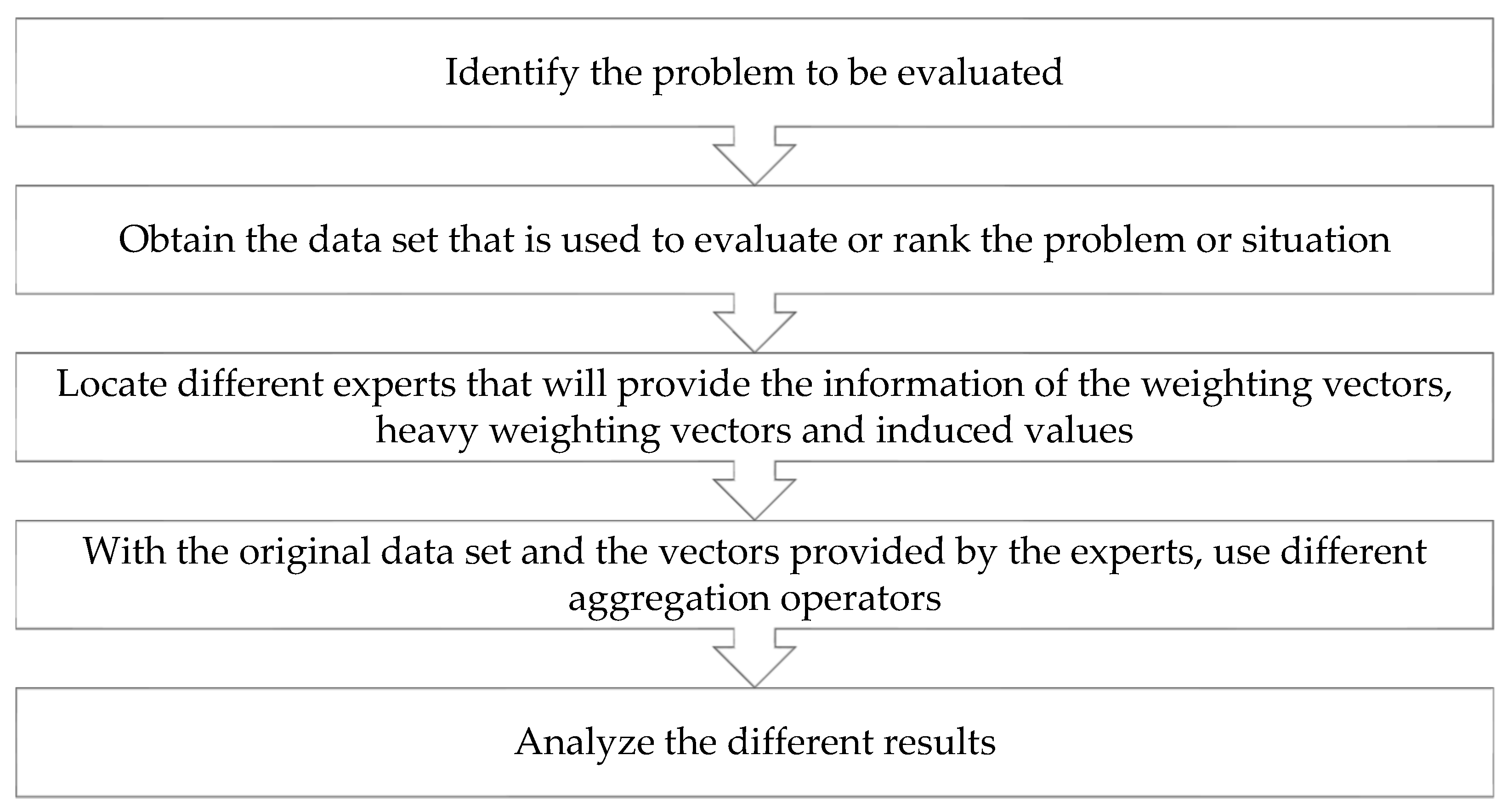
32	Chihuahua	30	12	0	0	45.45	17.49

. Finally, the steps to use the BON-PrOWA operator and other extensions are as follows.

Step 1. Locate different experts that give information regarding each of the components of the ranking of transparency websites. The information that will be requested is (a) weights, (b) heavy weights and (c) induced values. The profile of the experts for this article was as follows: (a) they had minimum of five years of experience within the government sector, specifically in areas related to transparency; and (b) they work or worked directly with government transparency websites.

Step 2. With the information provided by each expert, generate different classifications using the BON-OWA, BON-IOWA, BON-HOWA and BON-IHOWA operators.

Step 3. With the results obtained in Step 3, unify the information of the different experts based on the BON-PrOWA, BON-PrIOWA, BON-PrHOWA and BON-PrIHOWA operators, where the results of each expert are given a specific weight according to their experience in the field.

Step 4. Finally, the results are compared and analyzed.

To more clearly visualize the process to obtain the results, a simplified graph is presented (see Figure 1).

4.2. Evaluation of the Determinants of Transparency

Step 1. The information was provided by five experts. The conditions for being selected were as follows: (a) must be an active worker in an institution related to transparency and (b) must have more than 10 years in a similar position. The information provided by the experts is given in

Table 1. Weights provided by the experts.

Expert	Institutional Arrangements $({\mathit{c}}_1)$	Open Data $({\mathit{c}}_2)$	Vertical Collaboration $({\mathit{c}}_3)$	Horizontal Collaboration $({\mathit{c}}_4)$	Interface $({\mathit{c}}_5)$
$e_1$	0.15	0.30	0.20	0.20	0.15
$e_2$	0.10	0.20	0.30	0.30	0.10
$e_3$	0.10	0.30	0.25	0.25	0.10
$e_4$	0.15	0.15	0.30	0.20	0.20
$e_5$	0.10	0.15	0.30	0.30	0.15

,

Table 2. Heavy weights (heavy weights are the weights that will be used to calculate the heavy ordered weighted average (HOWA) operator. Their difference with the weights in Table 1 is that heavy weights are not bounded to ${\displaystyle \sum }_{j=1}^n{w}_j=1$; in this sense, the weighting vector can be from $1\le {\displaystyle \sum }_{j=1}^n{w}_j\le n$) provided by the experts.

Expert	Institutional Arrangement $({\mathit{c}}_1)$	Open Data $({\mathit{c}}_2)$	Vertical Collaboration $({\mathit{c}}_3)$	Horizontal Collaboration $({\mathit{c}}_4)$	Interface $({\mathit{c}}_5)$
$e_1$	0.20	0.30	0.20	0.20	0.20
$e_2$	0.15	0.20	0.30	0.30	0.15
$e_3$	0.10	0.30	0.30	0.30	0.10
$e_4$	0.20	0.20	0.30	0.20	0.20
$e_5$	0.10	0.20	0.30	0.30	0.20

and

Table 3. Induced values provided by the experts. Induced values are the values that will be used in the induced ordered weighted average (IOWA) operator, instead of a reordering step based on the value of the arguments, in this case, will be based on the induced value determined by the experts, generating a different reordering between the arguments and the weights. Also, the weights used in the Bonferroni induced ordered weighted average (Bon-IOWA) and Bonferroni prioritized induced ordered weighted average (Bon-PIOWA) operators are from Table 1 and for the Bonferroni induced heavy ordered weighted average (Bon-IHOWA) and Bonferroni prioritized induced heavy ordered weighted average (Bon-PIHOWA) operators are from Table 2.

Expert	Institutional Arrangements $({\mathit{c}}_1)$	Open Data $({\mathit{c}}_2)$	Vertical Collaboration $({\mathit{c}}_3)$	Horizontal Collaboration $({\mathit{c}}_4)$	Interface $({\mathit{c}}_5)$
$e_1$	5	2	1	3	4
$e_2$	4	2	1	3	5
$e_3$	3	2	1	4	5
$e_4$	5	4	2	3	1
$e_5$	5	2	3	1	4

.

Step 2. With the information provided in Step 1, generate the results using the BON-OWA, BON-IOWA, BON-HOWA and BON-IHOWA operators to understand the process that has been performed. An example using the information of expert 1 for the state of Zacatecas will be explained in detail, assuming that the process will be the same for all other states and experts. The values of q and p are equal to 1.

The first thing is determine the vectors $V^i$, and the results are

$$\begin{gathered} V_1=\left(90, 56, 85.71, 60\right) \\ {V}_2=\left(56, 85.71, 60, 100\right) \\ {V}_3=\left(85.71, 60, 100, 90\right) \\ {V}_4=\left(60, 100, 90, 56\right) \\ {V}_5=\left(100, 90, 56, 85.71\right) \end{gathered}$$

Next, the BON-OWA operator is applied. Then, a weight is assigned to each attribute according to a maximum criterion, and the results are

$$\begin{gathered} V_1=\left[\left(90\times 0.30)+\left(56\times 0.15\right)+\left(85.71\times 0.20\right)+(60\times 0.20\right)\right]=64.54 \\ {V}_2=\left[\left(56\times 0.15+ 85.71\times 0.20+ 60\times 0.20+100\times 0.30\right)\right]=67.54 \\ {V}_3=\left(85.71\times 0.15+ 60\times 0.15+ 100\times 0.20+ 90\times 0.20\right)=59.86 \\ {V}_4=\left(60\times 0.15+ 100\times 0.30+ 90\times 0.20+ 56\times 0.15\right)=65.40 \\ {V}_5=\left(100\times 0.30+90\times 0.20+ 56\times 0.15+ 85.71\times 0.15\right)=69.26 \\ BON-OWA={\left(\frac{\left[\left(64.54\times 100\right)+\left(67.54\times 90\right)+\left(59.86\times 56\right)+\left(65.40\times 85.71\right)+\left(69.26\times 60\right)\right]}{5}\right)}^{\frac{1}{1+1}} \\ BON-OWA=71.62 \end{gathered}$$

All the results for each state and expert are presented in

Table A2. Bon-OWA operator results.

States	${\mathit{e}}_1$	${\mathit{e}}_2$	${\mathit{e}}_3$	${\mathit{e}}_4$	${\mathit{e}}_5$
Zacatecas	71.62	72.77	72.60	71.12	72.47
Oaxaca	67.75	70.10	69.48	67.75	69.63
Nuevo Leon	66.19	68.30	67.87	66.23	68.02
Puebla	63.93	65.61	65.20	64.03	65.41
Nayarit	59.85	61.66	61.31	59.93	61.38
San Luis Potosí	60.08	62.46	61.73	60.46	62.25
Tlaxcala	58.40	60.19	59.86	57.93	59.80
Sonora	57.06	58.27	58.03	56.72	58.05
Yucatán	56.74	59.01	58.63	56.68	58.48
Querétaro	55.72	56.81	56.61	55.45	56.61
Quintara Roo	53.38	54.43	54.15	53.54	54.28
Estado de México	50.73	51.93	51.52	51.09	51.85
Guanajuato	48.68	50.56	50.14	48.53	50.26
Michoacán	47.66	49.94	49.18	47.95	49.67
Sinaloa	46.95	48.07	47.98	46.59	47.67
Coahuila	44.58	48.27	46.95	45.40	47.98
Veracruz	44.81	47.80	46.97	45.00	47.31
Baja California	44.02	45.53	45.23	43.54	45.21
Morelos	42.22	42.51	42.46	42.08	42.45
Hidalgo	42.01	43.56	43.14	42.11	43.26
Colima	39.93	42.36	41.79	39.99	41.87
Jalisco	37.52	38.51	38.19	37.74	38.44
Baja California Sur	37.23	37.49	37.46	37.13	37.43
Tamaulipas	36.91	37.43	37.31	36.84	37.39
Chiapas	36.62	39.77	38.53	37.23	39.55
Durango	36.53	38.33	37.84	36.65	38.05
Guerrero	36.52	36.99	37.10	36.10	36.73
Tabasco	35.23	37.63	37.01	35.34	37.24
Campeche	31.78	34.34	33.39	32.22	34.12
Aguascalientes	21.89	23.15	22.91	21.81	22.92
Ciudad de México	20.31	21.63	21.30	20.37	21.39
Chihuahua	15.36	16.50	15.94	15.71	16.50

.

In the case of the calculation for the BON-IOWA operator, the vectors $V^i$ are the same as those used in the BON-OWA operator. The next step is the association of the weights with the attributes that in this case will be performed by using the induced variables instead of the values of the attributes. Here, the results for Zacatecas are the following.

$$\begin{gathered} V_1=\left[\left(90\times 0.20)+\left(56\times 0.30\right)+\left(85.71\times 0.20\right)+(60\times 0.15\right)\right]=64.11 \\ {V}_2=\left[\left(56\times 0.20)+\left(85.71\times 0.30\right)+\left(60\times 0.20\right)+(100\times 0.15\right)\right]=66.11 \\ {V}_3=\left[\left(85.71\times 0.20)+\left(60\times 0.20\right)+\left(100\times 0.15\right)+(90\times 0.15\right)\right]=59.86 \\ {V}_4=\left[\left(60\times 0.30)+\left(100\times 0.20\right)+\left(90\times 0.15\right)+(56\times 0.15\right)\right]=65.40 \\ {V}_5=\left[\left(100\times 0.20)+\left(90\times 0.30\right)+\left(56\times 0.15\right)+(85.71\times 0.15\right)\right]=68.26 \\ BON-IOWA={\left(\frac{\left[\left(64.11\times 100\right)+\left(66.11\times 90\right)+\left(59.86\times 56\right)+\left(65.40\times 85.71\right)+\left(68.26\times 60\right)\right]}{5}\right)}^{\frac{1}{1+1}} \\ BON-OWA=71.29 \end{gathered}$$

All the results for each state and expert are presented in

Table A3. Bon-IOWA operator results.

States	${\mathit{e}}_1$	${\mathit{e}}_2$	${\mathit{e}}_3$	${\mathit{e}}_4$	${\mathit{e}}_5$
Zacatecas	71.29	71.97	71.77	70.77	71.32
Oaxaca	67.53	69.53	67.46	67.52	68.72
Nuevo Leon	66.13	68.11	66.85	66.14	67.83
Puebla	63.90	65.38	64.43	63.98	65.08
Nayarit	59.74	61.54	60.43	59.78	61.24
San Luis Potosí	59.80	61.88	60.70	60.07	61.43
Tlaxcala	57.93	59.31	58.54	57.67	58.54
Sonora	56.88	57.56	57.31	56.59	57.04
Yucatán	55.93	58.85	56.73	56.21	58.31
Querétaro	55.67	56.30	55.99	55.41	55.88
Quintara Roo	52.82	54.14	53.45	53.10	53.81
Estado de México	49.96	51.48	50.88	50.07	51.20
Guanajuato	48.49	50.13	48.74	48.34	49.81
Michoacán	46.47	49.20	47.53	47.24	48.60
Sinaloa	45.80	47.60	46.52	45.98	46.98
Coahuila	43.93	47.11	45.50	44.54	46.54
Veracruz	43.18	47.20	44.29	44.16	46.46
Baja California	43.70	44.58	44.16	43.36	43.85
Morelos	41.93	42.27	42.14	41.81	42.09
Hidalgo	40.72	43.08	41.67	41.23	42.63
Colima	38.41	41.92	39.63	39.13	41.46
Jalisco	36.98	38.08	37.62	37.10	37.65
Baja California Sur	37.04	37.30	37.21	36.95	37.20
Tamaulipas	36.45	37.27	36.58	36.58	37.15
Chiapas	35.55	38.62	36.68	36.61	37.90
Durango	35.67	37.82	36.73	36.01	37.54
Guerrero	36.16	36.59	36.34	35.73	36.24
Tabasco	34.46	37.23	35.12	34.90	36.67
Campeche	30.78	33.48	31.76	31.64	32.91
Aguascalientes	21.72	22.88	22.31	21.66	22.76
Ciudad de México	19.62	21.41	20.10	20.01	21.08
Chihuahua	14.13	15.94	15.00	14.94	15.66

.

In the case of the BON-HOWA operator, the vectors $V^i$ are also the same, but the weights will the ones presented in Table 2 and will be ordered with the arguments with a maximum criterion. Therefore, the results for Zacatecas are the following.

$$\begin{gathered} V_1=\left[\left(90\times 0.30)+\left(56\times 0.20\right)+\left(85.71\times 0.20\right)+(60\times 0.20\right)\right]=67.34 \\ {V}_2=\left[\left(56\times 0.20)+\left(85.71\times 0.20\right)+\left(60\times 0.20\right)+(100\times 0.30\right)\right]=70.34 \\ {V}_3=\left[\left(85.71\times 0.20)+\left(60\times 0.20\right)+\left(100\times 0.20\right)+(90\times 0.20\right)\right]=67.14 \\ {V}_4=\left[\left(60\times 0.20)+\left(100\times 0.30\right)+\left(90\times 0.20\right)+(56\times 0.20\right)\right]=71.20 \\ {V}_5=\left[\left(100\times 0.30)+\left(90\times 0.20\right)+\left(56\times 0.20\right)+(85.71\times 0.20\right)\right]=76.34 \\ Bon-HOWA={\left(\frac{\left[\left(67.34\times 100\right)+\left(70.34\times 90\right)+\left(67.14\times 56\right)+\left(71.20\times 85.71\right)+\left(76.34\times 60\right)\right]}{5}\right)}^{\frac{1}{1+1}} \\ BON-HOWA=74.17 \end{gathered}$$

All the results for each state and expert are presented in

Table A4. Bon-HOWA operator results.

States	${\mathit{e}}_1$	${\mathit{e}}_2$	${\mathit{e}}_3$	${\mathit{e}}_4$	${\mathit{e}}_5$
Zacatecas	74.17	75.28	76.06	73.77	75.48
Oaxaca	69.82	72.11	73.16	69.82	72.25
Nuevo Leon	68.33	70.38	71.55	68.33	71.00
Puebla	66.24	67.86	68.66	66.35	68.28
Nayarit	61.82	63.57	64.61	61.88	64.08
San Luis Potosí	61.86	64.17	65.01	62.19	64.60
Tlaxcala	59.95	61.70	62.77	59.53	62.01
Sonora	59.00	60.17	60.86	58.68	60.45
Yucatán	58.05	60.26	61.68	58.09	60.66
Querétaro	57.74	58.79	59.44	57.49	59.05
Quintara Roo	55.30	56.31	56.78	55.48	56.49
Estado de México	52.43	53.59	53.96	52.73	53.81
Guanajuato	50.00	51.84	52.81	49.85	52.23
Michoacán	48.60	50.83	51.55	48.96	51.03
Sinaloa	48.10	49.20	50.09	47.85	49.31
Coahuila	44.96	48.62	49.55	45.74	48.97
Veracruz	45.09	48.07	49.30	45.40	48.33
Baja California	45.07	46.54	47.39	44.61	46.77
Morelos	43.98	44.26	44.44	43.85	44.33
Hidalgo	42.90	44.42	45.09	43.05	44.50
Colima	40.18	42.61	43.81	40.35	42.85
Jalisco	38.71	39.67	39.99	38.92	39.87
Baja California Sur	38.79	39.04	39.24	38.70	39.12
Tamaulipas	38.30	38.80	39.07	38.35	39.00
Chiapas	36.80	39.93	40.51	37.44	40.08
Durango	37.15	38.92	39.69	37.31	39.16
Guerrero	37.66	38.11	38.77	37.27	38.27
Tabasco	35.56	37.94	39.00	35.76	38.24
Campeche	31.94	34.49	35.08	32.42	34.64
Aguascalientes	22.19	23.44	24.16	22.11	23.72
Ciudad de México	20.45	21.76	22.36	20.56	21.89
Chihuahua	15.36	16.50	16.50	15.71	16.50

.

Finally, the BON-IHOWA operator is constructed. The vectors $V^i$ are the same as the other operators, but the weights will be the ones in Table 2 and will be ordered based on the induced values of Table 3 The results for Zacatecas are the following.

$$\begin{gathered} V_1=\left[\left(90\times 0.20)+\left(56\times 0.30\right)+\left(85.71\times 0.20\right)+(60\times 0.20\right)\right]=66.91 \\ {V}_2=\left[\left(56\times 0.20)+\left(85.71\times 0.30\right)+\left(60\times 0.20\right)+(100\times 0.20\right)\right]=68.91 \\ {V}_3=\left[\left(85.71\times 0.20)+\left(60\times 0.20\right)+\left(100\times 0.20\right)+(90\times 0.20\right)\right]=67.14 \\ {V}_4=\left[\left(60\times 0.30)+\left(100\times 0.20\right)+\left(90\times 0.20\right)+(56\times 0.20\right)\right]=71.20 \\ {V}_5=\left[\left(100\times 0.20)+\left(90\times 0.30\right)+\left(56\times 0.20\right)+(85.71\times 0.20\right)\right]=75.34 \\ BON-IHOWA={\left(\frac{\left[\left(66.91\times 100\right)+\left(68.91\times 90\right)+\left(67.14\times 56\right)+\left(71.20\times 85.71\right)+\left(75.34\times 60\right)\right]}{5}\right)}^{\frac{1}{1+1}} \\ BON-IHOWA=73.86 \end{gathered}$$

All the results for each state and expert are presented in

Table A5. Bon-IHOWA operator results.

States	${\mathit{e}}_1$	${\mathit{e}}_2$	${\mathit{e}}_3$	${\mathit{e}}_4$	${\mathit{e}}_5$
Zacatecas	73.86	74.63	75.21	73.44	74.75
Oaxaca	69.61	71.57	70.72	69.60	71.66
Nuevo Leon	68.27	70.27	70.30	68.25	70.88
Puebla	66.21	67.66	67.71	66.29	68.06
Nayarit	61.71	63.50	63.56	61.73	63.99
San Luis Potosí	61.58	63.69	63.89	61.81	64.08
Tlaxcala	59.50	60.93	61.38	59.28	61.21
Sonora	58.83	59.57	60.06	58.55	59.80
Yucatán	57.25	60.18	59.78	57.64	60.55
Querétaro	57.69	58.33	58.68	57.45	58.58
Quintara Roo	54.76	56.16	56.24	55.06	56.19
Estado de México	51.69	53.40	53.62	51.73	53.39
Guanajuato	49.82	51.55	51.14	49.67	51.94
Michoacán	47.43	50.21	50.19	48.26	50.33
Sinaloa	46.98	48.80	48.95	47.26	48.86
Coahuila	44.31	47.68	48.12	44.89	48.04
Veracruz	43.47	47.51	46.90	44.56	47.78
Baja California	44.75	45.69	46.23	44.44	45.91
Morelos	43.71	44.10	44.22	43.59	44.10
Hidalgo	41.64	44.18	44.02	42.19	44.10
Colima	38.68	42.34	42.00	39.49	42.58
Jalisco	38.19	39.47	39.61	38.30	39.36
Baja California Sur	38.61	38.96	39.03	38.52	38.98
Tamaulipas	37.86	38.75	38.42	38.11	38.85
Chiapas	35.73	38.84	38.81	36.82	39.00
Durango	36.31	38.68	38.82	36.68	38.83
Guerrero	37.31	37.87	38.04	36.91	37.95
Tabasco	34.79	37.56	37.09	35.32	37.87
Campeche	30.94	33.70	33.63	31.84	33.85
Aguascalientes	22.03	23.33	23.51	21.96	23.62
Ciudad de México	19.77	21.56	21.27	20.21	21.69
Chihuahua	14.13	15.94	16.06	14.94	15.94

.

Step 3. With all the results obtained in Step 2, the results for the BON-POWA, BON-PIOWA, BON-PHOWA and BON-PIHOWA operators can be obtained. The weights associated with each expert are the following: $e_1=0.30$, $e_1=0.10$, $e_1=0.20$, $e_1=0.15$ and $e_1=0.25$. The result for each operator for Zacatecas is as follows.

$$\begin{gathered} BON-POWA=\left[\left(71.62\times 0.30\right)+\left(72.77\times 0.10\right)+\left(72.60\times 0.20\right)+\left(71.12\times 0.15\right)+\left(72.47\times 0.25\right)\right]=72.07 \\ BON-PIOWA=\left[\left(71.29\times 0.30\right)+\left(71.97\times 0.10\right)+\left(71.77\times 0.20\right)+\left(70.77\times 0.15\right)+\left(71.32\times 0.25\right)\right]=71.39 \\ BON-PHOWA=\left[\left(74.17\times 0.30\right)+\left(75.28\times 0.10\right)+\left(76.06\times 0.20\right)+\left(73.77\times 0.15\right)+\left(75.48\times 0.25\right)\right]=74.93 \\ BON-PIHOWA=\left[\left(73.86\times 0.30\right)+\left(74.63\times 0.10\right)+\left(75.21\times 0.20\right)+\left(73.44\times .15\right)+\left(74.75\times 0.25\right)\right]=74.37 \end{gathered}$$

The results for all the states are presented in

Table A6. Results of prioritized Bonferroni operators.

States	Bon-POWA	Bon-PIOWA	Bon-PHOWA	Bon-PIHOWA
Zacatecas	72.07	71.39	74.93	74.37
Oaxaca	68.80	68.01	71.32	70.54
Nuevo Leon	67.20	66.90	69.85	69.53
Puebla	64.74	64.46	67.41	67.13
Nayarit	60.72	60.44	63.13	62.83
San Luis Potosí	61.25	60.64	63.46	62.91
Tlaxcala	59.15	58.30	61.14	60.41
Sonora	57.57	57.03	59.80	59.35
Yucatán	57.77	57.02	59.65	58.93
Querétaro	56.19	55.81	58.47	58.14
Quintara Roo	53.89	53.37	56.02	55.60
Estado de México	51.34	50.62	53.24	52.68
Guanajuato	49.53	49.01	51.28	50.77
Michoacán	48.74	47.60	50.07	49.11
Sinaloa	47.39	46.45	48.87	48.07
Coahuila	46.40	45.31	47.37	46.43
Veracruz	46.20	44.77	47.08	45.80
Baja California	44.64	43.87	46.04	45.38
Morelos	42.33	42.03	44.17	43.93
Hidalgo	42.72	41.70	43.91	43.07
Colima	41.04	39.88	41.84	40.81
Jalisco	38.02	37.40	39.38	38.91
Baja California Sur	37.34	37.13	38.97	38.81
Tamaulipas	37.15	36.75	38.69	38.35
Chiapas	38.14	36.83	38.77	37.64
Durango	37.37	36.62	38.36	37.73
Guerrero	36.67	36.19	38.02	37.61
Tabasco	36.35	35.49	37.18	36.38
Campeche	33.01	31.90	33.57	32.62
Aguascalientes	22.47	22.21	23.08	22.84
Ciudad de México	20.92	20.32	21.34	20.79
Chihuahua	15.93	14.99	16.04	15.27

.

4.3. Discussion of the Results

After an analysis of the different results obtained and presented in Table A2, Table A3, Table A4, Table A5 and Table A6, the main changes that are found are as follows.

Based on the top 10 results of the different aggregation operators and experts, the first four positions do not change at all with the different aggregation operators and experts. In this sense, even when the importance of each component varies, the four best states remain the same: Zacatecas, Oaxaca, Nuevo Leon and Puebla. Then, according to the aggregation operator and expert that we analyze, the ranking can change. For example, in ranks five and six, we usually find the states of San Luis Potosi and Nayarit, respectively, but with the use of the BON-IHOWA operator, the positions change to Nayarit and San Luis Potosi, respectively. The other remaining positions vary, but the states remain the same and are Tlaxcala, Sonora, Yucatan and Queretaro.

Based on the bottom 10 results, the first four positions (as in the case of the top 10) remain the same considering the different aggregation operators and experts. In this sense, the worst states are Chihuahua, Ciudad de Mexico, Aguascalientes and Campeche. Then, the fifth and sixth positions are Tabasco and Guerrero depending on the aggregation operator and expert. Finally, positions seven to ten can change drastically. For example, for expert 1, from the BON-OWA operator, Chiapas is considered among the bottom 10 states and Jalisco is not; however, according to the information provided by expert 2, Jalisco is among the bottom 10 and Chiapas is not. This is important because in this process, it is possible to see that depending on the importance that is given to the information, the states can be or cannot be in the bottom 10 list.

The same analysis can be performed for the states in the middle of the ranking, and they change positions based on the different experts and aggregation operators. First, the top 10 of the lists does not change at all, but it is possible to see some notable changes as the ones explained in the bottom 10 analysis. This information is important for policymakers and governments to analyze to change and implement public policies according to the deficiency of each state, which can vary depending on the importance given to the components. Additionally, as seen, the ranking changes, and the benefits and government support for the states can be rearranged because of their positions in the ranking.

5. Conclusions

The main objective of this document is to present the new BON-PrIHOWA operator. The main features of this new proposition are that one can combine a nonrestricted to one weighting vector, an induced vector that assigns weights to the attributes and a prioritized vector that unifies the opinions of the decision makers in a group decision-making process, where not all stakeholders have the same importance in the computation.

Additionally, in this document, the main definitions of the BON-PrIHOWA operator are included, and it is important to mention that the BON-PrIHOWA can be reduced to the PrIOWA, PrHOWA, IHOWA, and OWA. This is suggested when the complexity of the problem is minimal and not very extensive. However, the design of this operator, its functionality and its operability are intended for complex phenomena with highly dynamic information. This is the case, e.g., when a combination of expert information is required to assess open government initiatives and public policies.

The complete design of the BON-PrIHOWA operator uses a ranking of transparency websites for Mexico. Among the main results, it was possible to identify that the top and bottom four states remained the same even when the weights, operators and experts changed. This is important because their positions cannot change easily. However, other positions can also change drastically depending on the operator or expert and, because of that, the perception of transparency of the citizens and governors. The main component that changes the ranking is the importance that is given to each component of transparency websites. When the weights assigned to each result are not $\frac{1}{n}$, but rather they depend on the focus and goals of each government, the score can change drastically. This change in the weights is important because not all information can be treated in the same way since the characteristics, objectives and goals of the states are not always the same. They are derived from their demographic, economic, and geographic characteristics, among others, in such a way that treating similar information is not appropriate. The idea of identifying changes in the ranking can improve the public policies that are established because the ranking can be established not only by using the average of the components but also by using a specific operator depending on the individual characteristics of the state.

For future research, more extensions of the OWA operator can be conceived with the use of distance operators [43], Bonferroni means [17,29,44], moving averages [45,46,47,48], forgotten effects [47,49], the least square deviation [50,51] or logarithmic operators [52,53]. This is important when the subjectivity and the uncertainty of the decision–making process are presented. With the use of aggregation operators and other fuzzy techniques, it is possible to generate new scenarios based on the expertise and expectations of the decision makers. Additionally, the use of different coefficients to test the similarity between the rankings will be useful to compare rankings in decision-making fields [54]. Finally, these new techniques can be applied in different areas such as economics, finance, engineering, social science and other areas [55] where the idea and characteristics of fuzzy logic and fuzzy sets can be used [56,57].

References

1. OECD. Open Government: The Global Context and the Way Forward; Organisation for Economic Co-operation and Development: Paris, France, 2016. [Google Scholar]
2. OECD. Government at a Glance 2019; OECD Publishing: Paris, France, 2019. [Google Scholar]
3. Jaeger, P.T.; Bertot, J.C. Transparency and technological change: Ensuring equal and sustained public access to government information. Gov. Inf. Q. 2010, 27, 371–376. [Google Scholar] [CrossRef]
4. Abu-Shanab, E.A. Reengineering the open government concept: An empirical support for a proposed model. Gov. Inf. Q. 2015, 32, 453–463. [Google Scholar] [CrossRef]
5. Nam, T. Challenges and concerns of open government: A case of government 3.0 in Korea. Soc. Sci. Comput. Rev. 2015, 33, 556–570. [Google Scholar] [CrossRef]
6. Piotrowski, S.J.; Van Ryzin, G.G. Citizen attitudes toward transparency in local government. Am. Rev. Public Adm. 2007, 37, 306–323. [Google Scholar] [CrossRef]
7. McDermott, P. Building open government. Gov. Inf. Q. 2010, 27, 401–413. [Google Scholar] [CrossRef]
8. Meijer, A.; ’t Hart, P.; Worthy, B. Assessing government transparency: An interpretive framework. Adm. Soc. 2018, 50, 501–526. [Google Scholar] [CrossRef] [Green Version]
9. Héritier, A. Composite democracy in Europe: The role of transparency and access to information. J. Eur. Public Policy 2003, 10, 814–833. [Google Scholar] [CrossRef]
10. Gupta, A. Transparency in Global Environmental Governance: A Coming of Age? MIT Press: Cambridge, MA, USA, 2010. [Google Scholar]
11. Piotrowski, S.J.; Zhang, Y.; Lin, W.; Yu, W. Key issues for implementation of Chinese open government information regulations. Public Adm. Rev. 2009, 69, S129–S135. [Google Scholar] [CrossRef]
12. Terrazas-Tapia, R. IDAIM 2014. Índice del Derecho de Acceso a la Información de México; Fundar, Centro de Análisis e Investigación: Mexico City, Mexico, 2014. [Google Scholar]
13. INAI. Informe de Labores. Utilidad del Acceso a la Información; Instituto Nacional de Transparencia, Acceso a la Información y Protección de Datos Personales: Mexico City, Mexico, 2019. [Google Scholar]
14. Sandoval-Almazán, R. Midiendo al gobierno abierto en México: Los portales estatales de transparencia durante el periodo 2015–2016. Transparencia Combate a la Corrupción y Gobierno Abierto La Experiencia en México 2017, 29, 47–66. [Google Scholar]
15. Beliakov, G.; Pradera, A.; Calvo, T. Aggregation Functions: A Guide for Practitioners; Springer: Heidelberg, Germany, 2007; Volume 221. [Google Scholar]
16. Yager, R.R.; Kacprzyk, J.; Beliakov, G. Recent Developments in the Ordered Weighted Averaging Operators: Theory and Practice; Springer: Berlin/Heidelberg, Germany, 2011; Volume 265. [Google Scholar]
17. Bonferroni, C. Sulle medie multiple di potenze. Bollettino dell’Unione Matematica Italiana 1950, 5, 267–270. [Google Scholar]
18. Yager, R.R. On ordered weighted averaging aggregation operators in multicriteria decisionmaking. IEEE Trans. Syst. ManCybern. 1988, 18, 183–190. [Google Scholar] [CrossRef]
19. Yager, R.R. Prioritized OWA aggregation. Fuzzy Optim. Decis. Mak. 2009, 8, 245–262. [Google Scholar] [CrossRef]
20. Yager, R.R.; Filev, D.P. Induced ordered weighted averaging operators. IEEE Trans. Syst. ManCybern. Part B (Cybern.) 1999, 29, 141–150. [Google Scholar] [CrossRef] [PubMed]
21. Merigó, J.M.; Gil-Lafuente, A.M. The induced generalized OWA operator. Inf. Sci. 2009, 179, 729–741. [Google Scholar] [CrossRef] [Green Version]
22. Yager, R.R. Generalized OWA aggregation operators. Fuzzy Optim. Decis. Mak. 2004, 3, 93–107. [Google Scholar] [CrossRef]
23. Yager, R.R. Heavy OWA operators. Fuzzy Optim. Decis. Mak. 2002, 1, 379–397. [Google Scholar] [CrossRef]
24. Blanco-Mesa, F.; León-Castro, E.; Merigó, J.M. A bibliometric analysis of aggregation operators. Appl. Soft Comput. 2019, 81, 105488. [Google Scholar] [CrossRef]
25. Detyniecki, M.; Bouchon-meunier, D.B.; Yager, D.R.; Prade, R.H. Mathematical Aggregation Operators and Their Application to Video Querying. Ph.D. Thesis, Pierre and Marie Curie University, Paris, France, 2000. [Google Scholar]
26. Herrera, F.; Martínez, L. A 2-tuple fuzzy linguistic representation model for computing with words. IEEE Trans. Fuzzy Syst. 2000, 8, 746–752. [Google Scholar]
27. Yu, D. A scientometrics review on aggregation operator research. Scientometrics 2015, 105, 115–133. [Google Scholar] [CrossRef]
28. Rickard, J.T.; Aisbett, J. New classes of threshold aggregation functions based upon the Tsallis q-exponential with applications to perceptual computing. IEEE Trans. Fuzzy Syst. 2013, 22, 672–684. [Google Scholar] [CrossRef]
29. Blanco-Mesa, F.; Merigó, J.M.; Kacprzyk, J. Bonferroni means with distance measures and the adequacy coefficient in entrepreneurial group theory. Knowl. Based Syst. 2016, 111, 217–227. [Google Scholar] [CrossRef]
30. Blanco-Mesa, F.; Merigó, J.M. Bonferroni distances and their application in group decision making. Cybern. Syst. 2020, 51, 27–58. [Google Scholar] [CrossRef]
31. Blanco-Mesa, F.; León-Castro, E.; Merigó, J.M. Bonferroni induced heavy operators in ERM decision-making: A case on large companies in Colombia. Appl. Soft Comput. 2018, 72, 371–391. [Google Scholar] [CrossRef]
32. Blanco-Mesa, F.; León-Castro, E.; Merigó, J.M.; Xu, Z. Bonferroni means with induced ordered weighted average operators. Int. J. Intell. Syst. 2019, 34, 3–23. [Google Scholar] [CrossRef] [Green Version]
33. Blanco-Mesa, F.; León-Castro, E.; Merigó, J.M.; Herrera-Viedma, E. Variances with Bonferroni means and ordered weighted averages. Int. J. Intell. Syst. 2019, 34, 3020–3045. [Google Scholar] [CrossRef]
34. Blanco-Mesa, F.; León-Castro, E.; Merigó, J.M. Covariances with OWA operators and Bonferroni means. Soft Comput. 2020, 1–16. [Google Scholar] [CrossRef]
35. Perez-Arellano, L.A.; Leon-Castro, E.; Blanco-Mesa, F.; Fonseca-Cifuentes, G. The ordered weighted government transparency average: Colombia case. J. Intell. Fuzzy Syst. 2020, 1–13. [Google Scholar] [CrossRef]
36. Merigo, J.M.; Casanovas, M. Decision-making with distance measures and induced aggregation operators. Comput. Ind. Eng. 2011, 60, 66–76. [Google Scholar] [CrossRef] [Green Version]
37. Merigó, J.M.; Gil-Lafuente, A.M.; Gil-Aluja, J. A new aggregation method for strategic decision making and its application in assignment theory. Afr. J. Bus. Manag. 2011, 5, 4033–4043. [Google Scholar]
38. Yager, R.R. On generalized Bonferroni mean operators for multi-criteria aggregation. Int. J. Approx. Reason. 2009, 50, 1279–1286. [Google Scholar] [CrossRef] [Green Version]
39. Baez-Palencia, D.; Olazabal-Lugo, M.; Romero-Muñoz, J. Toma de decisiones empresariales a través de la media ordenada ponderada. Inquietud Empresarial 2019, 19, 11–23. [Google Scholar]
40. Yager, R.R. Prioritized aggregation operators. Int. J. Approx. Reason. 2008, 48, 263–274. [Google Scholar] [CrossRef] [Green Version]
41. Merigó, J.M.; Palacios-Marqués, D.; Soto-Acosta, P. Distance measures, weighted averages, OWA operators and Bonferroni means. Appl. Soft Comput. 2017, 50, 356–366. [Google Scholar] [CrossRef]
42. Blanco-Mesa, F.; Merigó, J.M.; Gil-Lafuente, A.M. Fuzzy decision making: A bibliometric-based review. J. Intell. Fuzzy Syst. 2017, 32, 2033–2050. [Google Scholar] [CrossRef] [Green Version]
43. Hamming, R.W. Error detecting and error correcting codes. Bell Syst. Tech. J. 1950, 29, 147–160. [Google Scholar] [CrossRef]
44. Espinoza-Audelo, L.F.; Olazabal-Lugo, M.; Blanco-Mesa, F.; León-Castro, E.; Alfaro-Garcia, V. Bonferroni Probabilistic Ordered Weighted Averaging Operators Applied to Agricultural Commodities’ Price Analysis. Mathematics 2020, 8, 1350. [Google Scholar] [CrossRef]
45. León-Castro, E.; Avilés-Ochoa, E.; Merigó, J.M.; Gil-Lafuente, A.M. Heavy Moving Averages and Their Application in Econometric Forecasting. Cybern. Syst. 2018, 49, 26–43. [Google Scholar] [CrossRef] [Green Version]
46. León-Castro, E.; Avilés-Ochoa, E.; Merigó, J.M. Induced heavy moving averages. Int. J. Intell. Syst. 2018, 33, 1823–1839. [Google Scholar] [CrossRef]
47. Olazabal-Lugo, M.; Leon-Castro, E.; Espinoza-Audelo, L.F.; Maria Merigo, J.; Gil Lafuente, A.M. Forgotten effects and heavy moving averages in exchange rate forecasting. Econ. Comput. Econ. Cybern. Stud. Res. 2019, 53. [Google Scholar] [CrossRef]
48. Kenny, J.F.; Keeping, E.S. Relative merits of mean, median, and mode. Math. Stat. Van Nostrans Nj (Ed) 1962, 211–212. [Google Scholar]
49. Alfaro Calderón, G.G.; Godinez Reyes, N.L.; Gómez-Monge, R.; Alfaro-García, V.G.; Gil Lafuente, A.M. Forgotten effects in the valuation of the social well-being index in Mexico’s sustainable development. Fuzzy Econ. Rev. 2019, 24, 67–81. [Google Scholar] [CrossRef]
50. Hong, D.H.; Han, S. The general least square deviation OWA operator problem. Mathematics 2019, 7, 326. [Google Scholar] [CrossRef] [Green Version]
51. Wang, Y.-M.; Luo, Y.; Liu, X. Two new models for determining OWA operator weights. Comput. Ind. Eng. 2007, 52, 203–209. [Google Scholar] [CrossRef]
52. Alfaro-García, V.G.; Merigó, J.M.; Gil-Lafuente, A.M.; Kacprzyk, J. Logarithmic aggregation operators and distance measures. Int. J. Intell. Syst. 2018, 33, 1488–1506. [Google Scholar] [CrossRef] [Green Version]
53. Zhou, L.G.; Chen, H.y. Generalized ordered weighted logarithm aggregation operators and their applications to group decision making. Int. J. Intell. Syst. 2010, 25, 683–707. [Google Scholar] [CrossRef]
54. Sałabun, W.; Urbaniak, K. A new coefficient of rankings similarity in decision-making problems. In Computational Science—ICCS 2020; ICCS 2020. Lecture Notes in Computer Science; Springer: Cham, Switzerland, 2020; pp. 632–645. [Google Scholar]
55. Blanco-Mesa, F. La ciencia de la decisión. Revista UIS Ingenierías 2020, 19, I–V. [Google Scholar] [CrossRef]
56. Zadeh, L.A. Fuzzy sets. Inf. Control. 1965, 8, 338–353. [Google Scholar] [CrossRef] [Green Version]
57. Zadeh, L.A. Fuzzy logic. Computer 1988, 21, 83–93. [Google Scholar] [CrossRef]
Figure 1. Flowchart of the steps to use the Bonferroni prioritized induced heavy ordered weighted average (BON-PIHOWA) operator.
Mathematics 09 00024 g001