Cluster Flows and Multiagent Technology

Abstract

Multiagent technologies provide a new way for studying and controlling complex systems. Local interactions between agents often lead to group synchronization, also known as clusterization (or clustering), which is usually a more rapid process in comparison with relatively slow changes in external environment. Usually, the goal of system control is defined by the behavior of a system on long time intervals. As is well known, a clustering procedure is generally much faster than the process of changing in the surrounding (system) environment. In this case, as a rule, the control objectives are determined by the behavior of the system at large time intervals. If the considered time interval is much larger than the time during which the clusters are formed, then the formed clusters can be considered to be “new variables” in the “slow” time model. Such variables are called “mesoscopic” because their scale is between the level of the entire system (macro-level) and the level of individual agents (micro-level). Detailed models of complex systems that consist of a large number of elementary components (miniature agents) are very difficult to control due to technological barriers and the colossal complexity of tasks due to their enormous dimension. At the level of elementary components of systems, in many applications it is impossible to verify the models of the agent dynamics with the traditionally high degree of accuracy, due to their miniaturization and high frequency of control actions. The use of new mesoscopic variables can make it possible to synthesize fewer different control inputs than when considering the system as a collection of a large number of agents, since such inputs will be common for entire clusters. In order to implement this idea, the “clusters flow” framework was formalized and used to analyze the Kuramoto model as an attracting example of a complex nonlinear networked system with the effects of opportunities for the emergence of clusters. It is shown that clustering leads to a sparse representation of the dynamic trajectories of the system, which makes it possible to apply the method of compressive sensing in order to obtain the dynamic characteristics of the formed clusters. The essence of the method is as follows. With the dimension N of the total state space of the entire system and the a priori assignment of the upper bound for the number of clusters s, only m integral randomized observations of the general state vector of the entire large system are formed, where m is proportional to the number s that is multiplied by logarithm $N/s$. A two-stage observation algorithm is proposed: first, the state space is limited and discretized, and compression then occurs directly, according to which reconstruction is then performed, which makes it possible to obtain the integral characteristics of the clusters. Based on these obtained characteristics, further, it is possible to synthesize mesocontrols for each cluster while using general model predictive control methods in a space of dimension no more than s for a given control goal, while taking the constraints obtained on the controls into account. In the current work, we focus on a centralized strategy of observations, leaving possible decentralized approaches for the future research. The performance of the new framework is illustrated with examples of simulation modeling.

1. Introduction

It is common in a sociological (or physical) investigation to differ amid three primary societal (or system) levels: the micro-level, the meso-level, and the macro-level. In sociology, the analysis deals with a person in a social context or with a small people unit in a particular social setting. The consequences across a large population that result in significant inner transmissions are a matter of the macro-level commonly associated with the so-named global level. In turn, a meso-level study is provided for groups lying in their size amid the micro and macro levels, and often explicitly invented in order to disclose relations between micro and macro levels. Following this general taxonomy, we can analogously consider the Information (Digital) Age (a famous appellation of the modern period) as the macro-level Industrial Revolution, expressed by a quick transmission from the traditional industry to the massive application of information technology. Thus, humanity reconsiders the old-fashioned machinery aiming for new manufacturing solutions for new, regularly arising problems. Modern technologies lead to difficult supplementary tasks in the “global balancing” in humans’ interactions and nature. Most people hardly comprehend their lifestyle undergo significantly modifying on the micro-level than the prior industrial standard of living. The majority barely seriously consider modern discoveries in natural sciences, such as in high-energy physics or cosmology. For instance, even though the quantum theory has proven itself to be essential in nanotechnology [1,2], as well as particle accelerators in tumor treatment [3], yet, for many people, these fundamental achievements remain “abstract nonsense”. Consecutively, the scientific community facing a severe problem cannot often deliver further strict theoretical evaluation regarding new previously unknown phenomena. It takes place due to the known crisis of the modern scientific look at the “picture of the world”. Aiming to handle this global difficulty, it seems reasonable to primarily pay attention to an appropriate theory that is based on a suitable mathematical model. Note that a real-world system often cannot be described sufficiently entirely with a partial model that raises the need to have one with the lowest potential bias. While discussing the model concept, it appears to be essential to mention such a notion as information. According to [4], data are inextricably presented as a reflection of a mutable object and it can be described through other primaries notions, such as “matter”, “structure”, or “system”. Information can be stored and transferred with a material carrier, giving a form further perceived. It should also be noted that such a data concept is dedicated (from a system) to be supplementarily exploited. Generally speaking, it is a complex of ideas and representations of patterns that are discovered by a person in the real world. Thus, one may visualize a typical personal information process, as follows:

• Data gathering.
• Data studying.
• Data linkage to knowledge.

Thus, a model is nothing else but a way of information processing to knowledge. It is important to note that the human "perception" is an uninterrupted procedure of data accumulating with an "integration" that is needed in order to attain the required awareness.

Now, the question is whether we can decompose the information process further. In fact, psychology and cybernetics make attempts to do so; however, the further it goes, the harder it is to track the relation between a complex cognitive system and its fundamental components.

1.1. A New Approach to Compression

We can uncover the common features and fundamental differences at the outset, when comparing Data and Control Science with Physics. The central distinction between them is that Control Science studies systems with different complexity levels, commonly perceiving it as a scale. While physics deals in some extent with various systems in space and time, expressed in scales, like “length”. For example, the galaxy is immense in its extent in space, and the brain is immense in the complexity of its inner performance. As co-existing measures, these gradations are indeed tools uniting Physics with Data and Control Science in comprehending the world around us. Following the conventional view of the history of the Universe, we can suggest that the initial chaos of elementary particles strives to arrange (clusterize) into the molecular connectivity studied by chemistry. This structure later led to the origin (clusterization) of life as a highly organized form of matter, studied by biology. The described clustering process is a subject of Control Science, which can seemingly connect the natural Sciences while studying each scale of complexity of the organization of matter from its own standpoint.

It appears that clustering: is closely related to a term lik “compression”. With the aim to understand compression, it is helpful to mention that a human usually is not capable of accumulating every detail in the personal sensory perception (registered by each cone and rod), but only the essential details. Such details could be considered to be clusterization of low-level data from the retina into high-level features. Moreover, the general tendency is to forget even these points, mainly due to the brain’s limited capabilities. Accordingly, the data are being distorted or lost, which leads to a deterioration in the quality of information recovery. In general, as it was discussed in [5], our mind quite often compresses data while using induction or deduction, in order to simplify information regarding the world.

This peculiarity of human perception is broadly exploited in computer systems. The famous Kotelnikov–Nyquist–Shannon sampling theorem [6,7] dictates the genaral rules of signal digitization, which allow for compressing continuous signal flow into a discrete set of numbers without a loss of information. However, this approach exhausts its limits over the years: it is exponentially harder to quantize signals when their dimensionality grows linearly, so that, where a 1-D signal requires ${10}^3$ samples to be preserved, a corresponding 2-D signal would require ${10}^6$ samples, not to mention the signals of higher dimensionality, which are being routinely transmitted today. Thus, compression algorithms are incredebly relevant nowadays, since they allow for speeding up information exchange at fixed bandwith: e.g., MP3 [8,9] allows for getting rid of unnecessary high sound frequencies in music, while JPEG [10,11] reduces the picture file size at the cost of coarsening high frequency components that are responsible for small details. In this way, a kind of compression is believed to occur in the flow of visual information (if we follow the most popular hypothesis) among the brain’s ventral and dorsal streams. However, such processes perform “on the fly” in the brain. On the other side, the computer can only manipulate preliminarly given data to be compressed.

Mathematically, a real-time compression can be understood as selecting essential parts of the surrounding big data containing the comprehensive information and then storing linear combinations of these parts (possibly with random weights). In order to implement this idea, a method like compressive sensing was proposed and discussed in [12,13,14]. In this paradigm, it is possible to compress a signal gradually, as it is read or perceived by a sensing system. Assume that a signal $f\in {\mathbb{R}}^N$ is s-sparse in some domain $\Psi \in {\mathbb{R}}^{N\times N}$, namely $f=\Psi x$, where x has, at most, s ($s\ll N$) non-zero elements (thus being called an s-sparse vector). In our interpretation, it means that, on some basis, the comprehensive information is stored in only s units of data out of N. Subsequently, compressive sensing can be described as:

$$y=\Phi \Psi x=Ax,$$

(1)

where $\Phi$ is an $m\times N(m\ll N)$ sampling matrix, A is the so-called measurement matrix, and $y\in {\mathbb{R}}^m$ is called the measurement vector or vector of compressed observations. Because $m\ll N$, the estimation of x by given y drives infinitely many solutions. However, in the case x is s-sparse, it becomes possible to reconstruct it without much loss of useful data with only $m\sim slog(N/s)$ variables being required. According to [12,13,14], amid the solutions of (1), we prefer those that maximize the number of zero elements in x. While one would be interested in minimizing an ${\ell }_0$ norm, as it provides the sparsest solution, this problem is NP-hard and a linear relaxation via the ${\ell }_1$ norm provides a good compromise between sparsity and computations complexity [12,15]. It is possible to compute ${\ell }_1$-optimized solution in polynomial time, using, for example, the interior-point method [16,17]. Optimization with the ${\ell }_1$ metric for the task of pattern recognition was first discussed in [18]. An optimal sparse ${\ell }_1$-stabilizing controller for a non-minimum phase system (a solution for the task of ${\ell }_1$-optimization in an infinite-dimensional space) was proposed in [19].

While the design of $\Phi$ is, in general, complicated, some randomized choices of $\Phi$ are possible according to the restricted isometry property (RIP) and minimization of incoherence [4]. It was shown that only $m=2cs{(logN)}^2,c>0$ measurements are sufficient for reconstructing x. In a special case when the elements $a_{ij}$ of A are identically independently distributed with respect to the normal distribution

$$a_{ij}\sim \mathcal{N}\left(0,\frac{1}{m}\right),$$

then $m=c_{1}slog(N/s)$ measurements are sufficient. In practice, it is known that $m\approx 4s$ measurements are often enough for the initial sparse data to be effectively reconstructed.

1.2. Multiagent Systems

Studied in Data and Control Science, the complexity levels in the matter’s configuration lead to the emergence of the "complex system" notion. It is important to note that the complexity is not ascribed to the system that is comprehended as a static object, but, to a greater extent, to the dynamic processes occurring within the system. They are the primary purpose of our research. A lack of computing power and limitations of the cognition methods encourage many severe difficulties in such research. In this regard, an approach that is intended to study a particular complex process resorts to various generalizations simplifying the considered task. For a while, systems that consist of numerous practically indistinguishable segments with obscure disordered interactions have only been statistically described. It appears to be impossible to describe the system’s overall behavior while using just macroscopic statistical characteristics of its composite elements. This approach can merely explain a minimal class of the perceived effects. While many complex systems properties may significantly disagree with relatively simple states of equilibrium or chaos, the statistical approaches deal with actually averaged or integrated subsystems. This circumstance can lead to the omission of important details, if, for example, the system forms a pattern or structure of clusters.

The above-described manifestation of the whole system properties that are not inherent to its separate elements is called emergence [20,21,22]. Indeed, any non-comprehended characteristic of a structure can be considered to be emergent. For example, if a person cannot understand why a car moves, then moving is understood as an emergent behavior of the system-the car. However, this process is undoubtedly well apprehended from an engineering standpoint of the smooth operations in the engine, transmission, and control system. Thus, emergence may turn out to be a common subjective misunderstanding, and it is quite another matter if the system’s behavior is a mystery beyond the capacity of any scientist. Say, consciousness is an emergent behavior of the brain from a naturalist’s point of view. To date, there are no apparent means for explaining the concept of consciousness itself resting upon just elements composing the brain. Moreover, even there is no way to check whether such a system is whatever cognizable with the help of somewhat arbitrarily powerful existing intelligence—or whether it is fundamentally, objectively unknowable. In the last case, the emergence is ostensive [21].

Assuming that the surrounded systems are still subjectively emergent, we can critically appraise the statistical methods that were applied to study complex systems. As an alternative to the accepted statistical methodology, the current article suggests an agent-based approach designed to overcome this practice’s limitations. In the agent-oriented framework, a complex system (called a multiagent system) is respected as an arrangement of basic independent elements (termed intelligent agents or just agents), which communicate to each other [23,24,25]. The current study intends to suggest a unified general theory connecting the macroscopic scale of the whole system and the individual components’ microscopic scale. It aims to understand the reasons for "complexity" occurring in multiagent networks. An expected result of such an approach consists of constructing managing multiagent systems (MAS) without an in-depth investigation of the agents’ profound nature.

The known belief–desire–intention model (BDI) of intelligent agents is a model of intelligent agents suggesting that each agent has a "convinced" achievable goal, including excitation of particular states, stabilization, or mutual synchronization. The latter of particular interest [26,27] subject is frequently associated with the agents’ self-organization in a network. The conception behindhand this consequence lies in the behavior of agents within a MAS. I.e., agents can regulate their internal states by exchanging messages that aim to form a system structure on a macroscopic scale. It is worth noting that a system can start from an arbitrary initial state, and not all agents are required to interact with others. These structures may include persistent global states (for example, task distribution in load balancing for a computer network [28]) or synchronized oscillations (Kuramoto networks [29]).

Because dynamic systems usually describe multiagent networks, the synchronization state signifies a convergence of dynamic trajectories to some unique synchronized one. This consequence is well studied in the case of linear systems [23,30,31]. The more general case of nonlinear control rules is first considered in [32], where the Kuramoto model of coupled oscillators is analyzed as an example of a system with nonlinear dynamics.

Cluster synchronization is a particular type of such procedures, which is essential in control tasks. The genuine compound of large-scale systems, like alliances of robots operating in a continuously changing setting, are frequently overly complicated to be regulated by traditional procedures, incorporating, for example, approximation by classical ODE models. However, sometimes, some groups in a population synchronize in clusters. The agents who fit in the same group are synchronized, but ones that belong to different groups are not. Because these clusters can be deemed to be separate variables, it is possible to significantly reduce the control system inputs.

Thus, we can now introduce three levels of complex multiagent systems: microscopic (the level of individual agents), mesoscopic (the level of clusters), and macroscopic (the level of the system as a whole). The following equation can write down the described relation

$$N\gg M>1,$$

(2)

where N is the number of agents and M is the number of clusters, which is supposed to be of the same order as the sparsity of the system.

In this paper, we reformalize the framework of multiagent networks proposed in [23] and refined in [32], aiming to apply compressive sensing for efficient observations of dynamic trajectories. For this purpose, in the current work, we propose an algorithm, on the first step of which the trajectories are quantized, then compressed. Afterward, we visualize the results and compare the quantized representations of the original state space with the reconstructed one. In some cases, the visual representation of the state space may lack contrast, especially when the resolution is quite high (the quantization step is low). For this issue to be resolved, some contrast enhancement techniques may be considered [33,34].

1.3. The Kuramoto Model

Y. Kuramoto [29] proposed a straightforward, yet versatile, nonlinear model of coupled oscillators for their oscillatory dynamics. Given a network of N agents (by $\mathcal{N}=\{1,\dots ,N\}$ here and further we denote a set of N agents), each with one degree of freedom frequently entitled a phase of an oscillator, the following system of differential equations describes its dynamics:

$${\dot{\theta }}_i\left(t\right)=w_i+\sum _{j=1}^N{K}_{ij}sin\left({\theta }_j\left(t\right)-{\theta }_i\left(t\right)\right),$$

(3)

where ${\theta }_i\left(t\right)$ is a phase of an agent-oscillator i, $K_{ij}$ is a weighted adjacency matrix of the network, and $w_i$ is an own (ingerent) frequency of an oscillator. Consistent with [35,36,37], agents move towards the position of frequency (${\dot{\theta }}_i={\dot{\theta }}_j\forall i,j\in \mathcal{N}$) or phase (${\theta }_i={\theta }_j\forall i$, $j\in \mathcal{N}$) synchronization below particular conditions on $w_i$ and $K_{ij}$.

Many generalizations of this model, like time-varying coupling constants (adjacency matrix $K_{ij}\left(t\right)$) and frequencies $w_i\left(t\right)$, are proposed [38]. The Kuramoto model with phase delays is considered in [39,40]. Furthermore, there exist extraordinary multiplex [41] or quantum [42] and cluster synchronization [43] variants of this model.

The mentioned model is an effective instrument for the cortical activity explanation in the human brain [41], exposing three brain activity types linking to three states of the Kuramoto network: unsynchronized, highly synchronized, and cluster synchronization. The methodology that is behind the model is also applied in robotics. Accordingly, in [44], the task of pattern formation on a circle using rules encouraged by it is presented. A paper [45] proposes an idea of an artificial brain that is based on the Kuramoto oscillators. In [32], cluster synchronization appearing in the discussed framework is examined in the multiagent systems context. Given the framework that we reformalize in the current paper, the restrictions for the clusterization to remain invariant were formulated. Thus, the simplicity and usefulness of this model caught our attention, so that we choose it further in order to demonstrate how compressive sensing can be applied to multiagent clustering.

2. Cluster Flows

The framework of cluster flows was first proposed in [23] and then supplemented by additional concepts and definitions in [32]. In the current work, we introduce this framework in the same form, as it is formulated in our previous article [32]. Thus, the definitions that we present in this paper strictly replicate those proposed in the mentioned previous works.

Intending to investigating the Kuramoto model, we discuss at the beginning general multiagent systems. Throughout, we consider non-isolated systems that consist of N agents, whose evolution is determined by their current state, their overall configuration, and the environment’s external influence. The following system of differential equations characterizes the dynamics of the agents’ interaction:

$$\dot{x_i}\left(t\right)=f_i(x_i\left(t\right),u_i\left(t\right),U_i\left(t\right),{\eta }_i\left(t\right)),$$

(4)

where t is unidirectional time, $x_i\left(t\right)\in {\mathbb{R}}^{n_i}$ is a so-called state vector of an agent $i\in \mathcal{N}$; $u_i\left(t\right)$ is a microscopic control input describing local interactions between agents; $U_i\left(t\right)$ is another function, which is responsible for macro- or mesoscopic control simultaneously affecting large groups of agents; and, ${\eta }_i\left(t\right)\in {\mathbb{R}}^{m_i}$ is an uncertain vector, which adds stochastic disturbances to the model. Despite that $u_i\left(t\right)$ and $U_i\left(t\right)$ can be included in the state vector of a system, it is essential to separate them from the state vectors for two reasons: in the context of information models, it is necessary to distinguish both the local process of communication ($u_i\left(t\right)$) and external effects ($U_i\left(t\right)$) that are usually caused by a macroscopic agent with an actuator, allowing to influence the whole system; more than that, it allows for clarifying the model itself. The state vector $x_i\left(t\right)$ may also have a continuous index, so that it becomes a field $x(t,a)$, where a is a continuous set of numbers. This could allow for reducing the summation to integration in some cases.

As it widely accepted, the topology of an agents’ network is presented by means of a directed interaction graph: $\mathcal{G}\left(t\right)=\left(\mathcal{N},\mathcal{E}\left(t\right)\right)$, where $\mathcal{N}$ is an agent vertex set and $\mathcal{E}\left(t\right)$ is the set of directed arcs. Introduce ${\mathcal{N}}_i\left(t\right)\subseteq \mathcal{N}$ as a time-dependent neighborhood of an agent i that consists of a set of in-neighbors of this agent. We further denote the in-degree of a vertex-agent i ($i\in \mathcal{E}$) by $d\left(i\right)={\sum }_{l=1}^N{a}_{il}$, where $a_{ij}$ are the elements of an adjacency matrix A of $\mathcal{G}$ (the sum of the weights of the corresponding arcs). Likewise, the in-degree of a vertex-agent i excluding j ($i,j\in \mathcal{E}$) is $d_j\left(i\right)={\sum }_{l=1,l\ne j}^N{a}_{il}$. A strongly connected graph is said to be if there is a directed path from any vertex-agent to every other one.

Our next purpose is to introduce two agents outputs, one intending to their communication and another evaluating the synchronization between agents. For this purpose, we associate with each agent i its output function $g_i$:

Definition 1.

A function $g_i(x_i\left(t\right),{\eta }_i\left(t\right))$ is called an output of an agent i if $g:{\mathbb{R}}^{n_i}\times {\mathbb{R}}^{m_i}\mapsto {\mathbb{R}}^l$, where l does not depend on i.

Onwards, we denote two outputs, the former of which is applied to the communication process, while the latter is responsible for measurement of inter-agent synchronization.

First, let $y_j\left(t\right)=g_j(x_j\left(t\right),{\eta }_j\left(t\right))j\in {\mathcal{N}}_i\left(t\right)$ be a communication output of an agent j from the neighborhood of i. We assume that the dynamics of an agent i at time t is affected by the outputs $y_j\left(t\right)$ of the agents j from its neighborhood. Further, we refer to this relation between agents as "coupling". In practice, the output data flow $y_i\left(t\right)$ can be transmitted from j to i or shown by the agent j and then identified by i. The exact transmission rules are usually outlined in $u_i$ (see (4)):

$$u_i\left(t\right)=f_i\left({\left\{y_j\left(t\right)\right\}}_{j\in {\mathcal{N}}_i\left(t\right)}\right),$$

(5)

where $f_i(·)$ depends on the outputs $y_j\left(t\right)j\in {\mathcal{N}}_i\left(t\right)$. The equation (5) provides control rules for i based on all outputs j recognized by i. With this regard, as in the network science and control theory, we call it a coupling protocol. Thus, we present the definition of a multiagent network, as in [32]:

Definition 2.

The triple consisting of (1) family of agents (see (4)); (2) interaction graph $\mathcal{G}$; and, (3) coupling protocol defined as in equation (5) is called a multiagent network.

Henceforth, we denote a multiagent network by the letter $\mathcal{N}$ and then sassociate it with its set of agents. Let $z_i\left(t\right)=h_i(x_i\left(t\right),{\eta }_i\left(t\right))$ be an output of an agent i, which we introduce for the measurement of synchronization.

Definition 3.

Let ${\Delta }_{ij}\left(t\right)=∥z_i\left(t\right)-z_j\left(t\right)∥$ stand for the deviation between outputs $z_i$ and $z_j$ at time t, where $∥·∥$ is a corresponding norm. Then:

1. 

agents i and j are (output) synchronized, or reach (output) consensus at time t if ${\Delta }_{ij}\left(t\right)=0$; similarly, agents i and j are asymptotically (output) synchronized if ${\Delta }_{ij}(\infty )={\overline{\lim }}_{t\to \infty }{\Delta }_{ij}\left(t\right)=0$; and,

2. 

agents i and j are (output) ε-synchronized, or reach (output) ε-consensus at time t if ${\Delta }_{ij}\left(t\right)\le \epsilon$; similarly, agents i and j are asymptotically (output) ε-synchronized if ${\Delta }_{ij}(\infty )={\overline{\lim }}_{t\to \infty }{\Delta }_{ij}\left(t\right)\le \epsilon$;

Summarizing the above, cluster synchronization of microscopic agents may lead to mesoscopic-scale patterns that are recognizable by a macroscopic sensor. However, there is no need to restrict those patterns to be static, since the most interesting cases appear when the patterns evolve and change in time. Such alterations may be caused either by external impacts, or as a result of critical changes inside the system.

Definition 4.

A family of subsets $\mathcal{M}\left(t\right)={\left\{{\mathcal{M}}_{\alpha }\left(t\right):{\mathcal{M}}_{\alpha }\left(t\right)\subseteq \mathcal{N}\forall t\ge 0\forall \alpha \in \overline{1,M\left(t\right)}\right\}}_{\alpha =1}^{M\left(t\right)}$ of $\mathcal{N}$ is told to be a time-dependent partition over $\mathcal{N}$ (in this work, time-dependent partition is also called just “partition” for the sake of simplicity) at time t if the following conditions are respected:

1. 

$\nexists {\mathcal{M}}_{\alpha }\left(t\right)\in \mathcal{M}\left(t\right):{\mathcal{M}}_{\alpha }\left(t\right)=⌀$;

2. 

${\bigcup }_{\alpha =1}^{M\left(t\right)}{\mathcal{M}}_{\alpha }\left(t\right)=\mathcal{N}\forall t\ge 0$; and,

3. 

${\mathcal{M}}_{\alpha }\left(t\right)\cap {\mathcal{M}}_{\beta }\left(t\right)=⌀\alpha \ne \beta$.

The following definition interprets cluster synchronization in terms of a set partition with conditions for the outputs $z_i\left(t\right)$.

Definition 5.

A multiagent network with a partition $\mathcal{M}\left(t\right)$ over $\mathcal{N}$ is (output) $(\epsilon ,\delta )$-synchronized, or reach (output) $(\epsilon ,\delta )$-consensus at time t for some $\delta \ge \epsilon \ge 0$ if

1. 

${\Delta }_{ij}\left(t\right)\le \epsilon$$i,j\in {\mathcal{M}}_{\alpha }\left(t\right)$${\mathcal{M}}_{\alpha }\left(t\right)\in \mathcal{M}\left(t\right)$ and

2. 

${\Delta }_{ij}\left(t\right)>\delta$$i\in {\mathcal{M}}_{\alpha }\left(t\right)$$j\in {\mathcal{M}}_{\beta }\left(t\right)$${\mathcal{M}}_{\alpha }\left(t\right)$, ${\mathcal{M}}_{\beta }\left(t\right)\in \mathcal{M}\left(t\right)\alpha \ne \beta$.

A $(0,0)$-synchronization is henceforth referred to as cluster synchronization. We also say that the $\mathcal{M}\left(t\right)$ is a clustering over $\mathcal{N}$.

Each cluster in a system with $M\left(t\right)$ clusters also has a set ${\overline{x}}_{\alpha },\alpha \in \overline{1,M\left(t\right)}$ of cluster integrals: such an approach is usually used for dimensionality reduction in physical models.

3. Compressive Sensing within the Kuramoto Model

The Kuramoto oscillator system with mesoscopic control function has been studied in paper [32] resting upon the canonical representation (4) and the proposed earlier definition of a multiagent network. Such a system can undertake cluster synchronization under certain conditions, as was demonstrated (see [32], Theorem 2). An appropriate simulation was also provided in order to illustrate this circumstance. We exploit these results in the subsequent consideration of compressive sensing.

3.1. Clusterization and Mesoscopic Control of the Kuramoto Model

Following the definition of a multiagent network, we introduce the connectivity graph between oscillator agent $\mathcal{G}=\left(\mathcal{N},\mathcal{E}\right)$ and suggest, for simplicity, that this graph is time-independent. The corresponding adjacency matrix is denoted by $\mathsf{{\rm Y}}$, an element ${\mathsf{{\rm Y}}}_{ij}$ of this matrix taking just values 0 and 1. The value 0 may be interpreted as “the agent j can not communicate to i ($j\notin {\mathcal{N}}_i$)”, while the value 1 means “signals from the agent j reach i ($j\in {\mathcal{N}}_i$)”. The communication between agents is implemented by transmitting their outputs $y_i\left(t\right)$ (see (5)) coinciding in this situation with the phase ${\theta }_i\left(t\right)$.

Let $\mathcal{M}\left(t_1\right)$ be a clustering of the system of oscillators at time t and do not let this clustering change over the interval $T=[t_1,+\infty )$ and $t\in T$. We introduce the following local and mesoscopic control functions:

$$\begin{array}{c}{u}_i\left(t\right)=w_i+\rho {\displaystyle \sum _{j\in {\mathcal{N}}_i}}{\mathsf{{\rm Y}}}_{ij}sin\left({\theta }_j\left(t\right)-{\theta }_i\left(t\right)\right),\\ U_i\left(t\right)={\mu }_i{\mathcal{F}}_{\alpha }(t,{\overline{x}}_{\alpha }),\end{array}$$

(6)

were $\rho >0$ is a constant, $w_i$—the own (natural) oscillator frequency ${\mathcal{F}}_{\alpha }(·)$—a mesoscopic function taking the same value for all elements in each cluster ${\mathcal{M}}_{\alpha }$, ${\mu }_i$ is the sensitivity of agent i to the control function ${\mathcal{F}}_{\alpha }(·)$. An additional argument ${\mathcal{F}}_{\alpha }(·)$ is ${\overline{x}}_{\alpha }\left(t\right)$ containing the integral characteristics of a cluster $\alpha$. It could be, for example, the position of the cluster centroid. Note that, in systems with a large number of agents in a cluster, its integral characteristics are weakly dependent on the state of individual agents.

Looking at the classical Kuramoto model (3), we can see that its right side is similar to the expression of a protocol in (6). In fact, we consider the right-hand side of (3) entirely as a protocol that corresponds to various adjacency matrices. For example, in the classical model (3), it is a weighted adjacency matrix K containing arbitrary real numerical values. We simplify the model by considering a binary adjacency matrix $\mathsf{{\rm Y}}$ that is multiplied by $\rho$. Thus, the Kuramoto model in the canonical multiagent representation with the addition of the meso-control function ($i\in {\mathcal{M}}_{\alpha }$) is:

$$\begin{array}{c}{\dot{\theta }}_i\left(t\right)={\mu }_i{\mathcal{F}}_{\alpha }(t,{\overline{x}}_{\alpha }\left(t\right))+w_i+\rho {\displaystyle \sum _{j\in {\mathcal{N}}_i\left(t\right)}}{\mathsf{{\rm Y}}}_{ij}sin\left({\theta }_j\left(t\right)-{\theta }_i\left(t\right)\right).\end{array}$$

(7)

Assume that the system has established a state of a cluster $(\epsilon ,\delta )$ synchronization. However, dynamics of some agents in the cluster ${\mathcal{M}}_{\alpha }$ under the control of $\mathcal{F}(·)$ can become "destructive" for the whole cluster in case the values of their sensitivity highly differ from those among the rest. Besides, a significant difference in the values of $w_i$ can also lead to undesirable effects, up to the chaotic behavior of the system. The following Theorem, which is also presented in [32], formalizes such scenarios by providing conditions for the model’s parameters that are sufficient for the $(0,0)$ cluster synchronization to remain.

Theorem 1.

Consider a multiagent network corresponding to (7). Let $t\in T$, output $z_i\left(t\right)={\dot{\theta }}_i\left(t\right)$, and ${\Delta }_{ij}\left(t\right)=\left|z_i\left(t\right)-z_j\left(t\right)\right|$. Let also ${\mathcal{F}}_{\alpha }$ does not depend on ${\theta }_i\forall i$. The following conditions are sufficient for this network to be output $(0,0)$-synchronized.

1. 

In case $i,j\in {\mathcal{M}}_{\alpha }$,

$$\left|w_i-w_j+({\mu }_i-{\mu }_j){\mathcal{F}}_{\alpha }\right|\le \rho C_{ij}\left(\sum _{l\in {\mathcal{N}}_i\left(t\right)}{\mathsf{{\rm Y}}}_{il}+\sum _{l\in {\mathcal{N}}_j\left(t\right)}{\mathsf{{\rm Y}}}_{jl}\right),$$

(8)

where $C_{ij}=1$ in case ${\mathsf{{\rm Y}}}_{ij}={\mathsf{{\rm Y}}}_{ji}=0$; otherwise,

$$C_{ij}=max\left\{\sqrt{1-{\left({\mathsf{\Gamma }}_i\left(j\right)\right)}^2},\sqrt{1-{\left({\mathsf{\Gamma }}_j\left(i\right)\right)}^2},\frac{\sqrt{2}}{2}\right\},$$

(9)

where

$${\mathsf{\Gamma }}_i\left(j\right)=\frac{-d_i\left(j\right)+\sqrt{{\left(d_i\left(j\right)\right)}^2+8{({\mathsf{{\rm Y}}}_{ij}+{\mathsf{{\rm Y}}}_{ji})}^2}}{4({\mathsf{{\rm Y}}}_{ij}+{\mathsf{{\rm Y}}}_{ji})}.$$

(10)

2. 

For $i\in {\mathcal{M}}_{\alpha }$, $j\in {\mathcal{M}}_{\beta }$, $\alpha \ne \beta$

$$|w_i-w_j+{\mu }_i{\mathcal{F}}_{\alpha }(t,{\overline{x}}_{\alpha })-{\mu }_j{\mathcal{F}}_{\beta }(t,{\overline{x}}_{\beta })|>0.$$

(11)

3. 

Graph $\mathcal{G}$ is strongly connected.

At the next step, we consider the simulations of the dynamic trajectories, together with the simulations of their mesoscopic observations that are based on compression sensing.

3.2. Algorithm of Compressive Sensing Application for Mesoscale Observations

Aiming to model the observations of the multiagent system by a data center, we similarly quantize its dynamic trajectories, as is done in the classical signal processing theory. With that being said, we heuristically bound and discretize the state space of the multiagent network of oscillators. Because the desired one-dimensional outputs are ${\left\{{\dot{\theta }}_i\left(t\right)\right\}}_{i\in \mathcal{N}}$, the corresponding dynamical trajectories lay on a coordinate plane with the horizontal axis being t and the vertical one being $\dot{\theta }$. We call the half-plane $t>0$ the whole state space, and denote it as $\mathfrak{S}$. Next, we wish to extract the bounded region of $\mathfrak{S}$ with corresponding infimum and supremum along $\dot{\theta }$, denoted as ${\dot{\Theta }}_{min}$ and ${\dot{\Theta }}_{max}$; at the same time, corresponding infimum and supremum along t are $t_{min}$ and $t_{max}$. Such a region is denoted $\mathfrak{R}$ and it is formally defined as $\mathfrak{R}=\left[{\dot{\Theta }}_{min},{\dot{\Theta }}_{max}\right)\times [t_{min},t_{max})\subset \mathfrak{S}$. Thus, for each $t\in T=[t_{min},t_{max})$, a point of a trajectory ${\dot{\theta }}_i\left(t\right)$ belongs to $\left[{\dot{\Theta }}_{min},{\dot{\Theta }}_{max}\right)$. The values of the infima and the suprema are such that all of the trajectories ${\left\{{\dot{\theta }}_i\left(t\right)\right\}}_{i\in \mathcal{N}}$ are contained within $\mathfrak{B}$ and they are visually resolvable on a plot. We choose not to include the suprema in $\mathfrak{R}$ for the sake of simplicity of the further notion.

In our case, the discretization of $\mathfrak{R}$ implies its splitting into cells (sampling):

$$\begin{array}{cc}\hfill \left[{\dot{\Theta }}_{min},{\dot{\Theta }}_{max}\right)& =\left[{\dot{\Theta }}_{min},{\dot{\Theta }}_1\right)\cup \dots \cup \left[{\dot{\Theta }}_{p-1},{\dot{\Theta }}_{max}\right),\hfill \\ \hfill {}_{min},t_{max})& =[t_{min},t_1)\cup \dots \cup [t_{q-1},t_{max}),\hfill \end{array}$$

(12)

where the values p and q are determined by sampling steps $ϵ={\dot{\Theta }}_i-{\dot{\Theta }}_{i-1}$ and $\tau =t_j-t_{j-1}$. In turn, the values of $ϵ$ and $\tau$ depend on the form of trajectories ${\left\{{\dot{\theta }}_i\left(t\right)\right\}}_{i\in \mathcal{N}}$ and they are chosen empirically. For example, the time $\tau$ should be much smaller than that during which a dynamical process of interest occurs. Such processes may include intra-cluster disturbances or inter-cluster flows of agents (cluster flows). Concerning $ϵ$, its value should be such that trajectories of agents from the same cluster lay in a single cell or, at least, in closely located ones. As for the agents from different clusters, their trajectories should be separated by a significant number of cells. Finally, we introduce matrix $\mathfrak{B}\in {\{0,1\}}^{p\times q}$ with an element $b_{i,j}$, being 1 in the case that at least a single trajectory lays in the cell $\left[{\dot{\Theta }}_{i-1},{\dot{\Theta }}_i\right)\times [t_{j-1},t_j)$; otherwise, this element equals 0.

Thus, the columns of $\mathfrak{B}$ are ready to be compressed according to (1). It is clear that, by choosing lower values of $ϵ$ and $\tau$, the dimensionality of $\mathfrak{B}$ increases, leading to an increase of resolution and "readability" of the corresponding discrete trajectory portrait. What is more important, the sparsity of $\mathfrak{B}$ would also increase, which could allow to apply compression more effectively, while preserving a decent amount of details.

The main sourse of "complexity" for such systems is the scale of its state space, thus data transmission from the micro-level to the macro-level might be a bottleneck in the whole pipeline of the communication process between the system and the data center. With that being said, we estimate the complexity of the proposed algorithm in terms of the amount of gathered data, rather than in terms of the classical asymptotic computational complexity. The classical approach to such a problem is to observe each agent among $\mathcal{N}$ separatedly or, if we reformulate this in relation to our method, to observe each segment of the quantized state space, as it was shown in [4]. Consider a column $b_{·j}$ of $\mathfrak{B}$, which is a vector in an p-dimensional space. Compressive sensing allows for reducing the amount of transmitted data from p to $slog(p/s)$, where s equals the number of non-zero components in the sparse signal that is represented by the vector $b_{·j}$. Thus, in the case of large state spaces compressive sensing allows to widen the mentioned bottleneck proportional to the sparsity for the mesoscopic control rules to be synthesized faster.

4. Simulations

The simulations are set up while using Python, as the simplicity of this programming language allows for us to focus on algorithms, rather than syntax. We have implemented the code in the Jupyter Notebook tool, where the visual representation of results interactively and consequently supports the corresponding blocks of code. The simulation environment can be found in the GitHub repository [46] and is free to use.

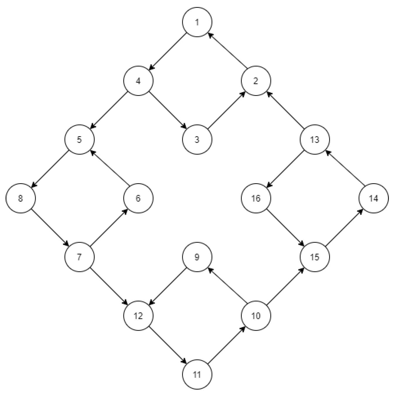
Consider model (7) and its solutions on $T=[0,60]$. Let the number of agents N be equal to 16, and the topology of connections between them be as on Figure 1. Despite that we choose N to be not quite large, its quantized state space appears to be of significant dimensionality, as it will be shown below. Such a state space may undoubtedly include a much larger amount of agents. However, after the cluster synchronization, they would occupy a relatively small zone (thus making the state space sparse), whether there are 16 or 1000 agents. With that being said, in the current work, we focus on a simple example just to demonstrate the main features of our approach.

Additionally, let the global connection strength $\rho =0.5$ and inherent frequencies ${\left\{w_i\right\}}_{i\in \mathcal{N}}$ be, as follows: $w_1,\dots ,w_4=\{4.1,4.2,4.3,4.4\},w_5,\dots ,w_8=\{8.1,\dots ,8.4\},w_9,\dots ,$ $w_{12}=\{12.1,\dots ,12.4\}$, $w_{13},\dots ,w_{16}=\{16.1,\dots ,16.4\}$, so that agents from one “square”-shaped component of the graph $\mathcal{G}$ (see Figure 1) satisfy the condition of the Theorem 1 manifested in (8). On the other hand, agents from different "squares" does not obey those conditions.

Assuming that the initial phases ${\theta }_i\left(0\right)$ are uniformly distributed on a circle $S^1$, in the absence of any mesoscopic control ($U_i=0$) and given that the outputs $z_i$ coincide with ${\dot{\theta }}_i$, the described configuration leads to cluster synchronization with a partition $\mathcal{M}$ consisting of four subsets of agents. 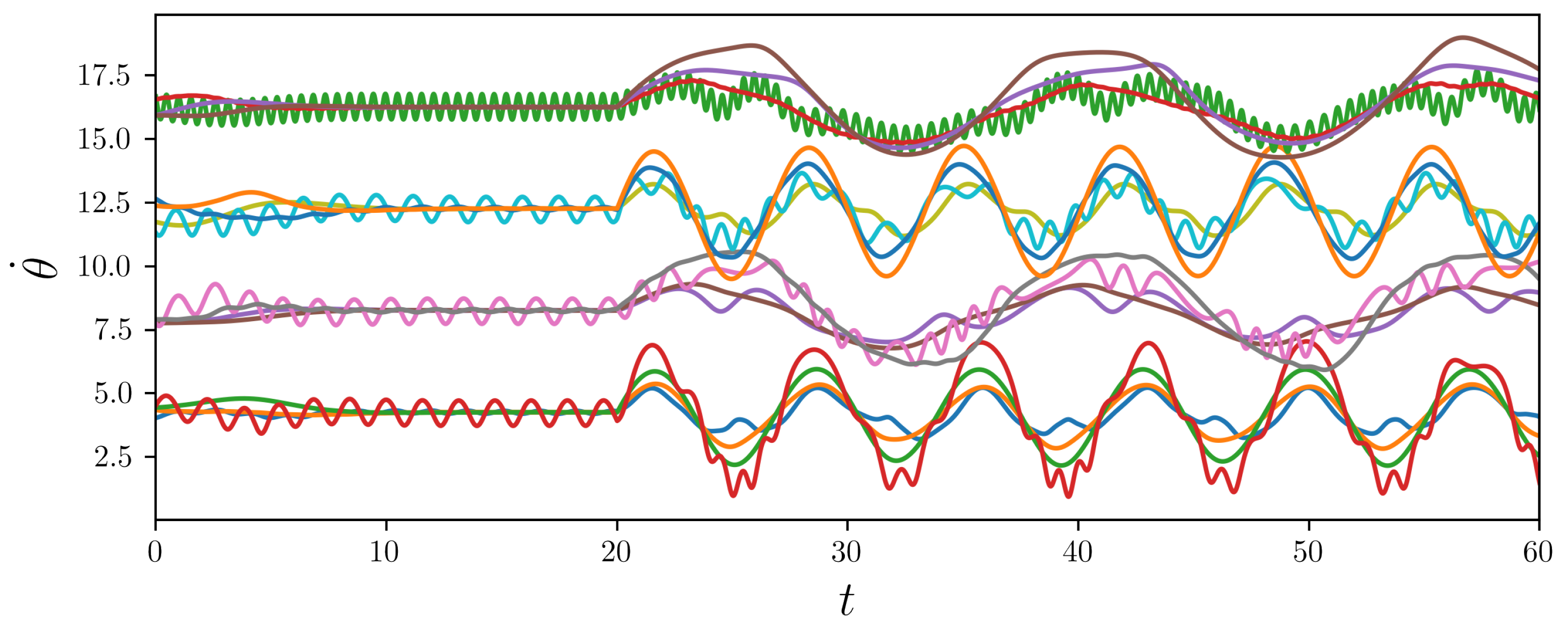In other words, we obtain $(\epsilon ,\delta )$-synchronized clusters for some values $\epsilon$ and $\delta$, such that $\epsilon \ll \delta$, which are analyzed in [32]. However, in this work, we focus on non-trivial “flowing” cluster patterns, which emerge after adding a sinusoidal control function $U_i\left(t\right)$ at $t\ge 20$, i.e., when $(\epsilon ,\delta )$-synchronization visually estabilish:

$$U_i={\mu }_i{\mathcal{F}}_{\alpha }(t,{\overline{x}}_{\alpha }\left(t\right))={\mu }_{i}sin\left(2\pi f_{\alpha }(t-20)\right),$$

where $f_{\alpha }$ are uniformly distributed on an interval $[0,1]$. We introduce the set of values ${\left\{{\mu }_i\right\}}_{i\in \mathcal{N}}$: $\{{\mu }_1,\dots ,{\mu }_4\}=\{{\mu }_5,\dots ,{\mu }_8\}=\{{\mu }_9,\dots ,{\mu }_{12}\}=\{{\mu }_{13},\dots ,{\mu }_{16}\}=\{0.625,1.25,1.875,2.5\}$. According to the Theorem 1 (see (8) and (11)), the assumed values of agents’ sensitivity may break cluster invariance. The simulated results that are illustrated in Figure 2 prove this statement to be correct.

We denote the parameters for quantization of the state space:

• ${\dot{\Theta }}_{min}=0$, ${\dot{\Theta }}_{max}=20$, $ϵ=0.02$; and,
• $t_{min}=20$, $t_{max}=60$, $\tau =0.1$.

The corresponding $1000\times 400$ matrix $\mathfrak{B}$ is constructed according to the algorithm described above and it is shown in Figure 3.

It turned out that $93\%$ of $\mathfrak{B}$’s elements are zero, so that its columns have sparse representation in the standard basis. We choose to compress the columns of $\mathfrak{B}$, since they represent the states of the considered systems observed during the time interval $[t_{i-1},t_i)$.

The next step is to generate $\Phi$, which is chosen to origin its elements from normal distribution $\mathcal{N}\left(0,\frac{1}{m}\right)$ (according to [4]), where m is the number of measurements, which we choose to be $2s$. We choose s to be the average number of non-zero elements among the columns of $\mathfrak{B}$. 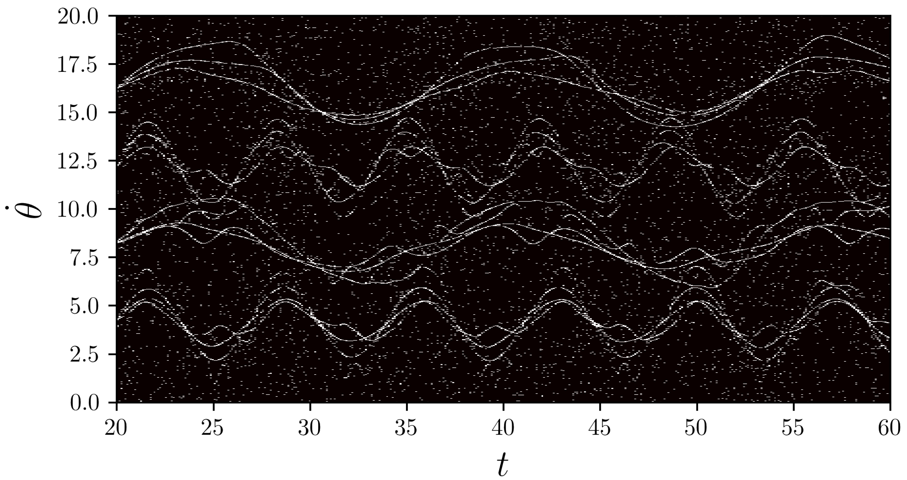As it will be shown in the image with reconstructed trajectories, the multiplier 2 is sufficient, despite that, in [4], it was equal to 4. This empirical decision can be justified by the fact that the dynamic trajectories have very sparse representation, unlike ordinary images. Thus, we provide decent compression for each column, reducing its length from 1000 to 139. Such data reduction brings us closely from the level of individual agents to the mesoscopic scale of clusters. A decompressed matrix $\overline{\mathfrak{B}}$ is obtained as a collection of restored columns as ${\ell }_1$-optimized vectors, numerically calculated with the interior-point method; it is shown in Figure 4. Despite that the decompressed matrix appears to be noisy, the overall features of the trajectories are still perceptable, which could inform us of the close to lossless compression.

5. Conclusions

We proposed a mathematical framework for the analysis of complex systems as multiagent networks. Besides, we proposed an algorithm of compressive sensing application for centralized observations of the agent trajectories, exploiting their sparsity in the discretized state space that is caused by clustering. We have also shown how this algorithm can be applied to the Kuramoto model: the achieved degree of compression could make it possible to efficiently transmit compressed state space data to a data center, where the results of cluster identification can be further handled by a control synthesis unit based on control methods with predictive models for a given control goal. Furthermore, we plan to consider a more in-depth study of compression in application to multiagent networks, which may bring us to the point of simple rules that link and explain all of the scales that complex systems operate on. For example, we are to consider decentralized multiagent strategies of data gathering. It would also be interesting to simulate systems that are composed of a huge amount of agents for better interpretation of the proposed method. We hope that our results would push further interest in researches regarding compressed observations of agent states for mesoscopic control.