1. Introduction
Over the last few years, an increasing number of research studies dealing with modeling of technological response variables as a function of process parameters in order to determine the most appropriate operating conditions has been observed in Manufacturing Engineering. Given the importance that these manufacturing processes have for industry, a large number of models have been developed in recent years, based on regression techniques, fuzzy inference systems, and artificial neural networks, generally through the application of supervised learning and feed forward networks. In this present research study, different techniques, based both on response surface methodology (RSM) and on soft computing, will be analyzed to determine their capacity to accurately predict the response variables. It should be noted that conventional regression techniques are effective when the models provide high values of the coefficient of determination. However, when the response variables have high curvature or are irregular, conventional models are not effective in modeling the response variables. Therefore, when regression models are not adequate to predict the behavior of the response variables, it is necessary to use other alternative methodologies and, as shown further on, soft computing has significant advantages over conventional regression methods.
In this present study, a comparative study is first carried out between the accuracy in regression models, based on RSM, versus that of soft computing techniques such as Artificial Neural Networks (ANN) and Adaptive Neuro-Fuzzy Inference Systems (ANFIS). First, from a Design Of Experiments (DOE), two sets of values generated from a function that can be made to exhibit both low curvature and high curvature within the range of variation of the DOE will be used, which is usually observed when modeling variables obtained in manufacturing processes where some part of them are well fitted by models obtained from regression, with high coefficients of determination, and some others, on the contrary, exhibit a behavior which is not possible to adequately model by using conventional regression techniques. Finally, a comparative analysis will be carried out between the results obtained with those that would be obtained in a real manufacturing study case and a comparison between those obtained will be carried out.
Furthermore, this comparison made between the regression and soft computing models does not use all the data from the DOE to fit the models, as is common practice. Instead, a part of the design is used to fit the model and another part for validation and testing, since the fact of using the entire DOE to fit the model does not allow its validation with independent data, and it may lead to results that are not completely reliable, as shown in this present study. Although it is true that there are different research studies that carry out comparative studies, the above-mentioned is not usually taken into consideration. In addition, this present study proposes a new methodology to obtain an ANFIS which is capable of efficiently modeling the response variables obtained from a DOE. An iteration with the membership functions is carried out to develop a Fuzzy Inference Systems (FIS) that will be tuned later by using an ANFIS. In this study, it will be shown that by using this method it is possible to efficiently model both response variables with low curvature and high curvature. The proposed method, which is shown is
Section 4.4, is based on finding the shape of the initial membership functions in order to develop a FIS which will be then tuned with an ANFIS and which will later lead to a better fit in the validation data as well as in the train data.
The results obtained by the different techniques are also compared. Before approaching the present study, several research works that were found in the bibliography will be analyzed in the “State of the Art” section.
2. State of the Art
Over the last few years, regression techniques as well as ANN, FIS, and ANFIS have been widely employed for modeling several manufacturing processes. In regard to FIS, these have been widely used in distinct scientific fields, among others, dealing with control, pattern recognition, and modeling [
1], where Takagi–Sugeno [
2,
3] and Mamdani [
4,
5] are the most commonly employed. Several studies can be found in the literature dealing with FIS, such as that of Mouralova et al. [
6] who proposed a Mamdani FIS for modeling the cutting speed in wire electrical discharge machining (WEDM). These authors employed a maximum of results for aggregation and the centroid to de-fuzzify the aggregated output. In another study, Aamir et al. [
7] used a Mamdani FIS to predict the surface roughness and hole size as a function of feed rate and cutting speed in multi-hole drilling. These authors calculated the outputs based on the centroid method. Some other studies are those of Cuka and Kim [
8] that developed a fuzzy inference system for tool condition monitoring in end-milling operations and Joshi et al. [
9] who analyzed surface roughness and material removal rate (MRR) of Inconel 800HT, when machined with copper electrode on electrical discharge machining (EDM). On the other hand, Wang et al. [
10] employed a fuzzy multicriteria decision-making model (MCDM) for raw material supplier selection in the plastic industry. Likewise, Lin et al. [
11] applied fuzzy collaborative intelligence approach for fall detection in four existing smart technology applications and a methodology for obtaining technological tables based on using a zero-order Sugeno FIS is shown in Ref. [
12]. Some other studies, worth mentioning, are those of Cavallaro [
13] that employed a Takagi–Sugeno FIS to assess the sustainability of biomass of production and that of Shabgard et al. [
14] who employed a Mamdani inference system to predict MRR, electrode wear and surface roughness in the EDM and ultrasonic-assisted EDM (US/EDM) processes of tungsten carbide.
Comparing the performance of different models for the prediction of response variables has been examined by different authors and for different variables and technological processes. For example, it is worth mentioning the research studies of Bernardos et al. [
15] which analyzed the arithmetic average roughness (Ra) in face milling using a feedforward ANN and a Levenberg–Marquardt algorithm. Furthermore, in the study of Devarasiddappa et al. [
16] these authors employed an ANN to predict surface roughness in WEDM of Inconel 825, and Twardowski et al. [
17] employed multilayer perceptron (MLP) for modeling tool wear during turning of hardened steel, among others. Another interesting technique for modeling technological variables in manufacturing processes are hybrid learning procedures that combine ANNs and FIS, which are known as ANFIS [
18]. ANN and Fuzzy systems are commonly combined in soft computing to solve real-world problems. From the research study of Jang [
18], several studies have been developed, as can be observed in the review of the state of the art of Shihabudheen and Pillai [
19]. For example, in Maher et al. [
20] an ANFIS was employed to predict cutting speed, surface roughness, and heat-affected zone in WEDM and in Çaydaş et al. [
21] an ANFIS was used for modeling surface roughness and white layer thickness in WEDM of an AISI D5 tool steel. Likewise, Kang et al. [
22] proposed a heating temperature estimation method for diagnosis and assessment of fire-damaged concrete structures by using an ANFIS. Al-Ghamdi [
23] employed an ANFIS and polynomial modeling approaches to model the MRR in EDM of a Ti-6Al-4V alloy. A first order Sugeno along with a back-propagation neural network training algorithm was used by these authors [
23]. Both ANNs and ANFIS have been widely used in Engineering and Technology fields, among many others. Comparison of ANFIS and MLP ANNs can be found in the bibliography dealing with different subjects. For example, in the study of Suparta et al. [
24] the authors employed both ANFIS and MLP for prediction of precipitable water vaper. These authors found that the ANFIS provided a better performance than that obtained by using MLP. On the other hand, in the research study of Yilmaz and Kaynar [
25] the authors employed multiple linear regression, ANN and ANFIS for prediction of swell percent of soil. These authors found that the ANN models had a better performance than that obtained with ANFIS and multiple regression.
Fuzzy modeling has been widely applied in several scientific and technological fields. There exists a large amount of industrial applications which are based on these techniques. Among the research studies found in the literature it is worth mentioning the application of soft computing techniques for airport classification, as shown in the research study of Postorino et al. [
26], control of piezoelectric actuators, as shown in Li et al. [
27] and in Cheng et al. [
28], control of Brushless DC motors [
29] and monitoring of fuel system of an industrial gas turbine, as shown in Bagua et al. [
30]. Other applications deal with both detection and classification of defects, as shown in Versaci [
31] and in Versaci et al. [
32], fault diagnosis of rolling bearing in industrial robots [
33], and fault detection in wind turbines [
34], among many others.
In addition, fuzzy systems are able to handle uncertainties in an efficient way, as shown in Lin et al. [
35], where a Takagi–Sugeno–Kang (TSK) type-2 fuzzy neural network was proposed for system modeling and noise cancellation, or in Biglarbegian et al. [
36], where a design methodology based on interval type-2 TSK fuzzy logic controllers for modular and reconfigurable robots manipulators with uncertain dynamic parameters was shown, among many others [
37,
38]. Furthermore, Chen et al. [
39] employed a type-2 fuzzy neural network to predict bearing health conditions and Tayyab et al. [
40] applied fuzzy theory to consider uncertainty in demand information in a multi-stage lean manufacturing system. These authors employed the centroid to de-fuzzify the objective function. Other studies such as that of Faisal et al. [
41] used particle swarm optimization (PSO) and biogeography-based optimization (BBO) algorithms for a multiple-objective optimization of the MRR and the arithmetical mean roughness (Ra) for the EDM process, Alarifi et al. [
42] employed genetic algorithms and particle swarm optimization to determine the parameters of an ANFIS model to predict the thermo-physical properties of Al
2O
3-MWCNT/thermal oil hybrid nanofluid and an analysis of the PSO implementation in designing parameters of manufacturing processes as well as a benchmark with other optimization techniques can be found in the review study of Sibalija [
43]. On the other hand, Alajmi et al. [
44] used an ANFIS-QPSO to predict the surface roughness of the dry and cryogenic turning process of AISI 304 stainless steel. Moreover, a comparison of prediction accuracy between ANFIS, ANFIS-GA, ANFIS-PSO, and ANFIS-QPSO was carried in this study in terms of the MAPE, root mean squared error (RMSE) and R
2 values for both dry and cryogenic turning processes [
44].
Furthermore, neural networks have also been widely employed in several scientific and technological fields. Among the research studies found in the literature it is worth mentioning the application of neural networks for prediction of biogases concentration using spiking neural networks [
45], feature recognition and process planning of casting dies [
46], quality control in manufacturing processes [
47], prediction of springback in sheet metal forming [
48], aerodynamic data modeling [
49], detection of skin diseases [
50], automatic control of house elements [
51,
52] and energy forecasting in the manufacturing sector [
53], among many other applications.
Finally, it is worth mentioning the employment of techniques based on the DOE and regression techniques that have also been widely used for the study of technological variables found in manufacturing processes as shown in research studies such as that of Airao et al. [
54] which analyzed the effect of cutting speed, feed rate, and axial depth of cut on surface roughness obtained in end-milling of a stainless steel, that of Kasdekara et al. [
55], which employed a 2
4 full factorial (DOE) for determining the most important factors which influence MRR in Electro-chemical machining of AA6061 by using MLP and regression, and that of Ahmed et al. [
56] in which the MRR, in laser milling of three alloys (Ti6Al4V, Inconel 718 and AA 2024), was evaluated using the response surface method and DOE. On the other hand, Aslantas et al. [
57] obtained empirical relations between cutting speed, feed rate, depth of cut and surface roughness parameters using the RSM for the micro-turning process in a Ti6Al4V alloy and Su et al. [
58] employed a multi-objective optimization method based on grey relational analysis and RSM along with Taguchi method for analyzing surface roughness and MRR in turning of an AISI 304 austenitic stainless steel. Regression analysis is also used by Zajac et al. [
59] to make predictions of cutting tool durability in turning processes. Furthermore, in the research study from Torres et al. [
60] the manufacturing of TiB
2 by using EDM was analyzed by using RSM. On the other hand, Torres at al. [
61] employed a 4
3 factorial DOE for modeling the behavior of the arithmetical mean roughness (Ra), the electrode wear (EW) and the MRR in the EDM machining of an Inconel
®600 alloy using Cu-C electrodes (Inconel®600 alloy is a registered trademark of the Special Metals Corporation group of Companies). In Lin et al. [
62] surface roughness in the end-milling process is analyzed as a function of spindle speed, cutting depth, and feed rate and machining vibration by using multiple regression and ANNs and in Karloopia et al. [
63] cutting speed, depth of cut, and feed are used as independent variables to obtain cutting force and tool wear in Al–Si–TiB2 composites by using linear regression.
As was observed in the “State of the Art” section, there are different methodologies that have been used for modeling technological variables in manufacturing processes, some of which will be analyzed in order to determine their performance in modeling response variables. The following section describes the methodology to be followed in this present study.
3. Methodology
As shown in the review of the state of the art, it is observed that regression models based on the use of experimental design have been widely employed for modeling the behavior of different technological variables, which in the manufacturing field, are usually related to surface finish, MRR, or tool wear, among many others. If there is enough data available, it would be considered interesting to validate the models with other independent experimental data to determine the validity of the fits. For this reason, the present study compares the results obtained when only one set of the DOE is used to train the model and the rest of the DOE is used to validate the obtained models, following the methodology that is employed in the Deep Learning Toolbox™ of Matlab
TM2019b [
64] to train, test, and validate ANNs and in order to compare the obtained results with both regression and soft computing tools (ANN and ANFIS).
Therefore, First, the data is randomly divided using the Matlab
TM2019b functions into three sets comprising 70%, 15%, and 15% of data (train, test, and validate, respectively). With the train data, a model will be fitted first, and then the thus obtained models will be validated using the validation data and later on they will be tested with independent test data [
64]. RSM as well as ANN, FIS, and ANFIS will be employed to analyze the advantages and disadvantages of each. Moreover, a method for obtaining and ANFIS from the DOE is proposed.
It should be mentioned that if the RSM model can provide a highly adjusted R-squared value, it could be considered in advance that it is not necessary to use soft computing techniques since they require higher computational time than the previous ones and, in general, the models thus obtained are more complex. However, if more precision is required or the response surface of a certain variable has a high curvature in the design range or if it is very irregular, this will make conventional regression models ineffective and lead to low values of the coefficient of determination to be obtained. Therefore, the use of some other types of techniques should be considered, such as those based on soft computing.
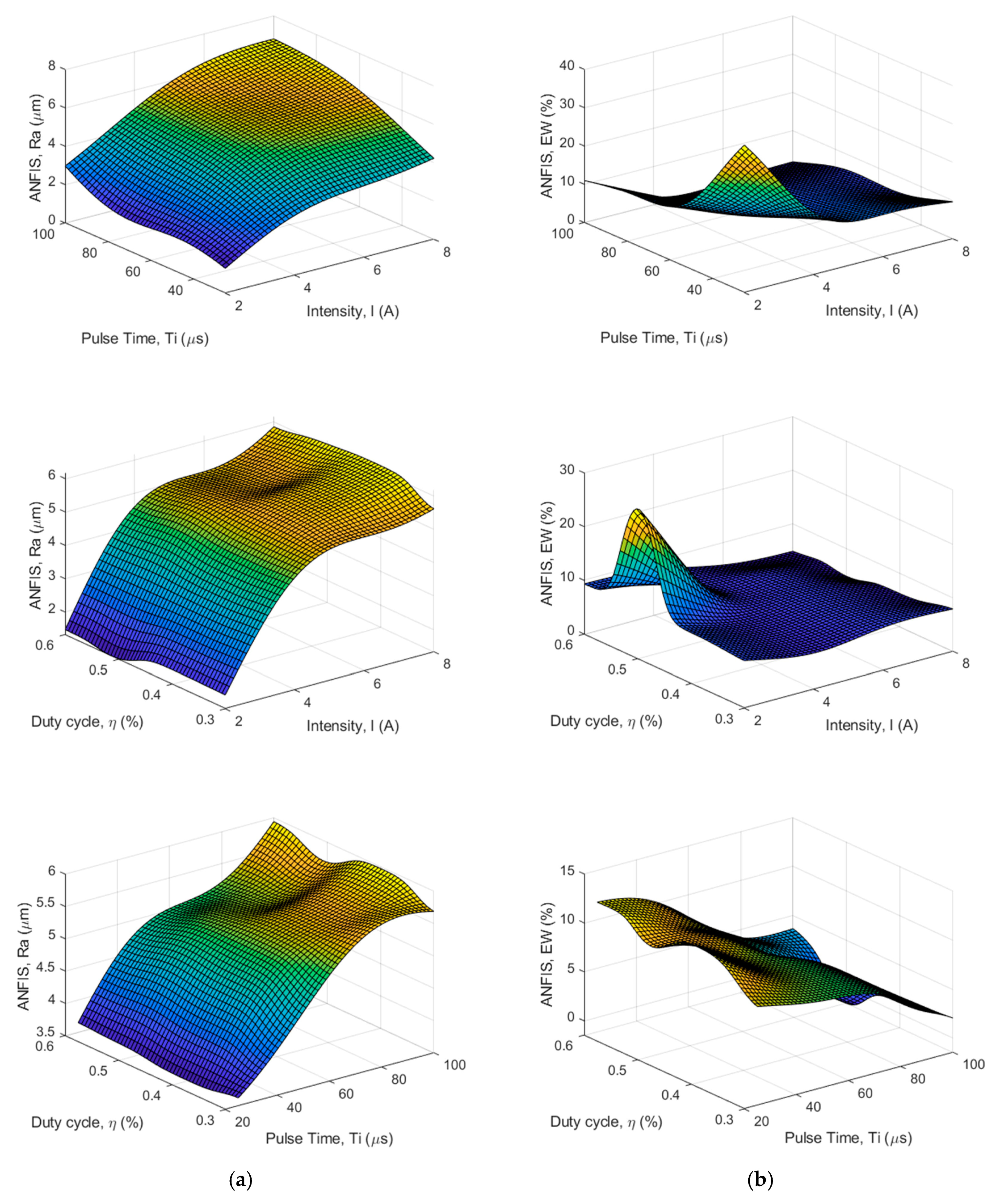
In manufacturing processes, is it quite common for certain technological variables to have a more regular response behavior and, therefore, they can be modeled by methodologies such as RSM, and, on the other hand, there also exist some other technological variables that cannot be adequately modeled using conventional regression techniques. For example, in Reference [
61] it is shown that the arithmetic average roughness (Ra) can be approximated by a polynomial regression using RSM, in an EDM process. However, due to the variability of the data, the wear that the electrode (EW) undergoes in this EDM process cannot be adequately modeled by using RSM, and for this reason, in order to adequately model this technological variable, it would be necessary to employ some other technique, for example based on using an ANFIS or an ANN. In this way, and using an ANFIS,
Figure 1a,b have been generated in order to show the surface responses that would be obtained when modeling Ra (µm) and EW (%), in the case of positive polarity of the electrode, using data taken from Ref. [
61]. As can be seen from the results shown in Ref. [
61], in which only RSM-based polynomial regression is used, the R-squared value is greater than 90% in the case of average roughness (Ra), but this coefficient is much lower in the case of EW and, hence, although Ra could be modeled by using RSM, this is not the case for the EW.
In this present study the function defined by Equation (1) will be used where their constants will be varied to have two types of response variables. This function has been chosen since it is possible to vary the values of the constant to have a function that shows a behavior that could be modeled properly by conventional regression techniques and can also be made to present a behavior with greater curvature, which is difficult to model by using the RSM methodology. The first type of response variable would represent the behavior of a response variable that has low curvature within the study range, which is to be classified as type 1 function , i.e., functions in which if the RSM is used in a set of data obtained from these functions, the adjusted coefficient of determination of the RSM regression models would provide values greater than 90%. Likewise, the second type of response variable would represent a behavior that either has a high curvature or where the experimental data are irregular in the design range considered, which may be classified as type 2 function .
As an example, from the determination coefficient of the regression shown in Ref. [
61], Ra (µm) surface response could be classified, from the previously mentioned, as type 1 function and EW (%) surface response could be classified as type 2 function. A DOE with three factors and four levels for each factor (3
4) will be used. This arrangement of the design is similar to that used in Ref. [
61]. However, any other type of DOE could be used. From this, the levels of the variables shown in
Table 1 are considered, where the levels of variation of the variables have been normalized to fall into the range
and the value obtained in the response variable will be left without normalizing it in order to directly obtain its value, without the need for a subsequent transformation. If necessary, a transformation of the dependent variable could also be performed so that it falls within a certain interval. Therefore, the
value corresponds to the minimum level of an input variable and the +1 value corresponds to the maximum value of this variable. It would be feasible to have any other range and to make a transformation to bring it to this range or to analyze it directly in the starting range.
The responses surfaces of the function considered in this present study are shown in
Figure 2. As can be observed,
Figure 2a presents a behavior that, in advance, could be considered to be adequately modeled by the RSM since it does not exhibit a great degree of curvature within the considered interval. On the contrary,
Figure 2b shows another function with a response surface in the considered interval which exhibits much greater curvature than the former.
It may be underlined that either an actual study case or any other function could have been used to carry out the first part of this study. As can be observed in
Figure 1 and
Figure 2, the response variables have similar shapes, for both study cases, i.e., low curvature in one response variable and high curvature in the other. Since a DOE has been used in accordance with that shown in
Table 1, therefore 4
3 experiments will be available. The values shown in
Table 2 and
Table 3 that have been generated from the previously mentioned functions, which are shown in
Figure 2, will be used in this study. To be consistent with the uncertainty of the measurements that the response variables may have, the values of the functions are considered to have been rounded to two decimal places.
As previously mentioned, in order to carry out the comparative study between the different models, data shown in
Table 2 and
Table 3 are randomly divided into three sets (train, test, validate) according to (70%, 15% and 15%). Thus, the experiments used to test and to validate the models are those corresponding to the positions {16, 17, 21, 22, 29, 32, 47, 51, 54, 62} and {2, 6, 20, 25, 35, 48, 49, 50, 52, 56}, respectively, the rest of the remaining experiments will be used to train the models. It should be noted that it would be possible to use all the points to train the models. However, it is considered that either some additional experiments or some points of the DOE should be used to validate the models, and hence this procedure has been followed in this study.
Once the methodology to be followed in this study as well as the classification proposed for the response variables (Types 1 and 2) has been shown, the results obtained by using the different methodologies for data modeling will be analyzed. Next, the validity of the results obtained with the analytical function will be compared with those obtained when a real case is studied. In addition, a new method for obtaining an ANFIS based on the train data and the validation data of the DOE will be shown in
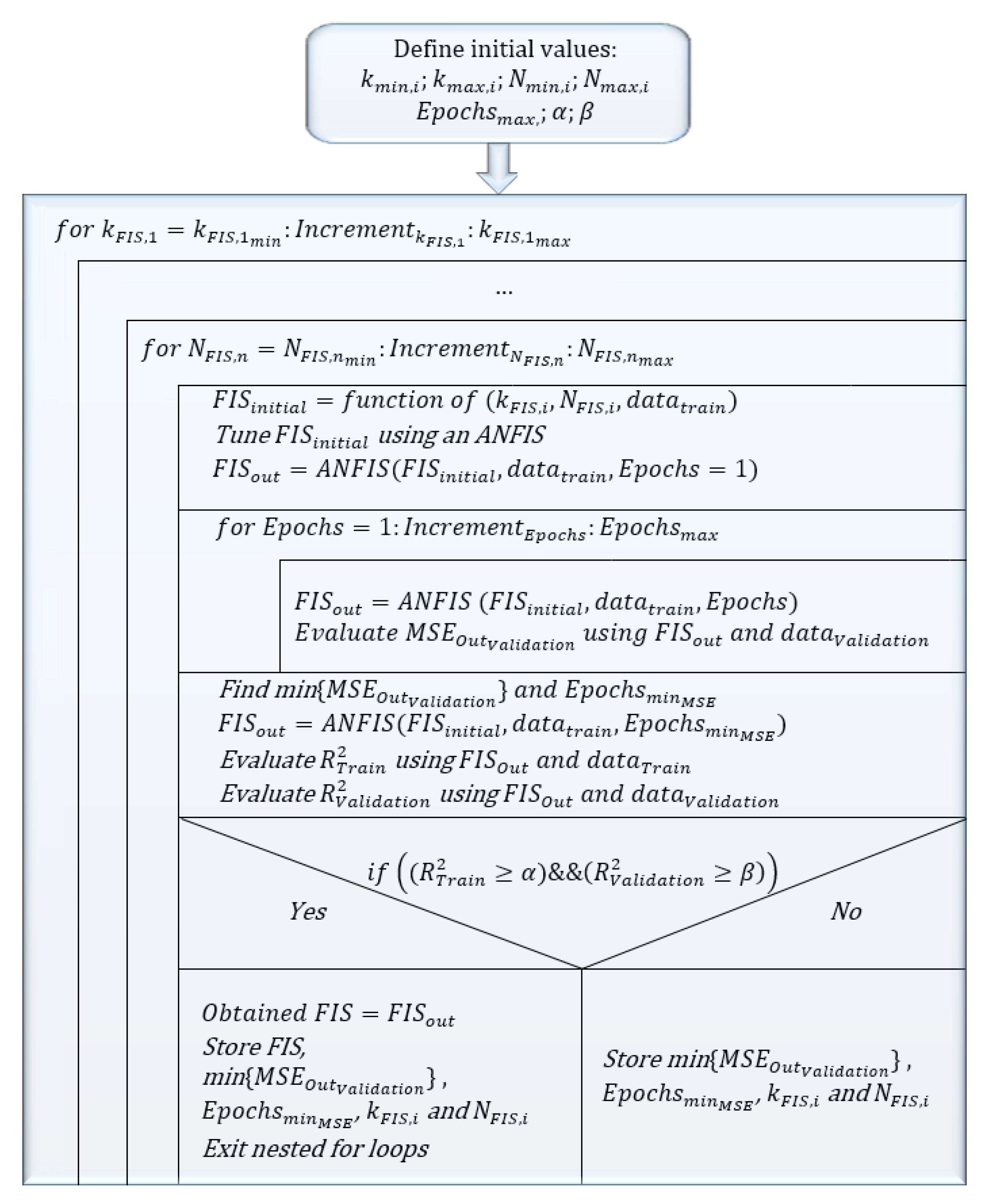
Section 4.4 and the obtained results will be compared. As previously mentioned, this proposed method is based on finding the shape of the initial membership functions in order to develop a FIS which will be then tuned with an ANFIS and in this way a better fit in the validation data as well as in the train data will be obtained.
Figure 3 shows a flowchart using a Nassi–Shneiderman diagram [
65] in order to introduce the algorithm of the proposed method, which will be analyzed in
Section 4.4 of this present study.
4. Results and Discussion
In this section, the results obtained when modeling the function shown in Equation (1) are shown which, as indicated, can present a behavior as shown in
Figure 2a that, in advance, could be expected that it will be adequately modeled by the RSM since it does not exhibit a great degree of curvature within the considered interval (type 1 function) and, on the contrary, it can be made to exhibit much greater curvature in the considered interval, as shown in
Figure 2b, and then it is likely that conventional regression techniques would not be adequate (type 2 function). Hence, some other types of technologies for data analysis should be used.
4.1. Response Surface Model (RSM)
Equation (2) shows the RSM to be used to predict the behavior of type 1 (
) and type 2 (
) functions, which are shown in
Figure 2a,b, by using data shown in
Table 2 and
Table 3, respectively.
Likewise, as previously mentioned,
Table 1 shows the levels of the independent variables analyzed in this study, where they are varied following a full factorial DOE.
Table 4 and
Table 5 show the results obtained by performing a regression fit using the train data included in
Table 2 and
Table 3 and by using the model shown in Equation (2). As can be observed, the regression coefficient of determination has a value of 0.961 and an adjusted R-squared value of 0.951, for the case of
function, which are high enough to be able to draw some conclusions from the regression models. However, in the case of
function, these values are much lower (0.577 and 0.465), respectively. For this reason, the model shown in Equation (2) is not as good as the first one for making predictions about the response variable. Therefore, it is necessary to use some other types of models that allow a better approximation to the actual behavior of the said variable to be obtained.
In this present study, instead of using the regression model obtained from the , the complete regression model will be used, which both considers all the effects of the variables in the models and has a higher value, since the fact of using the model adjusted to the degrees of freedom could eliminate some of the independent variables.
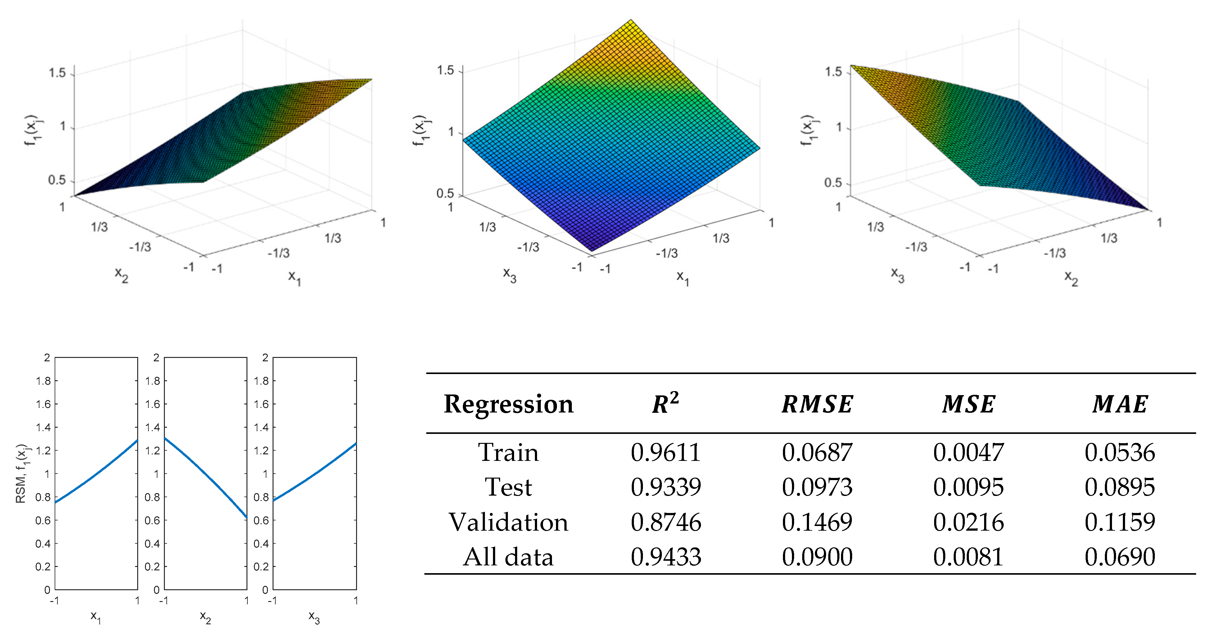
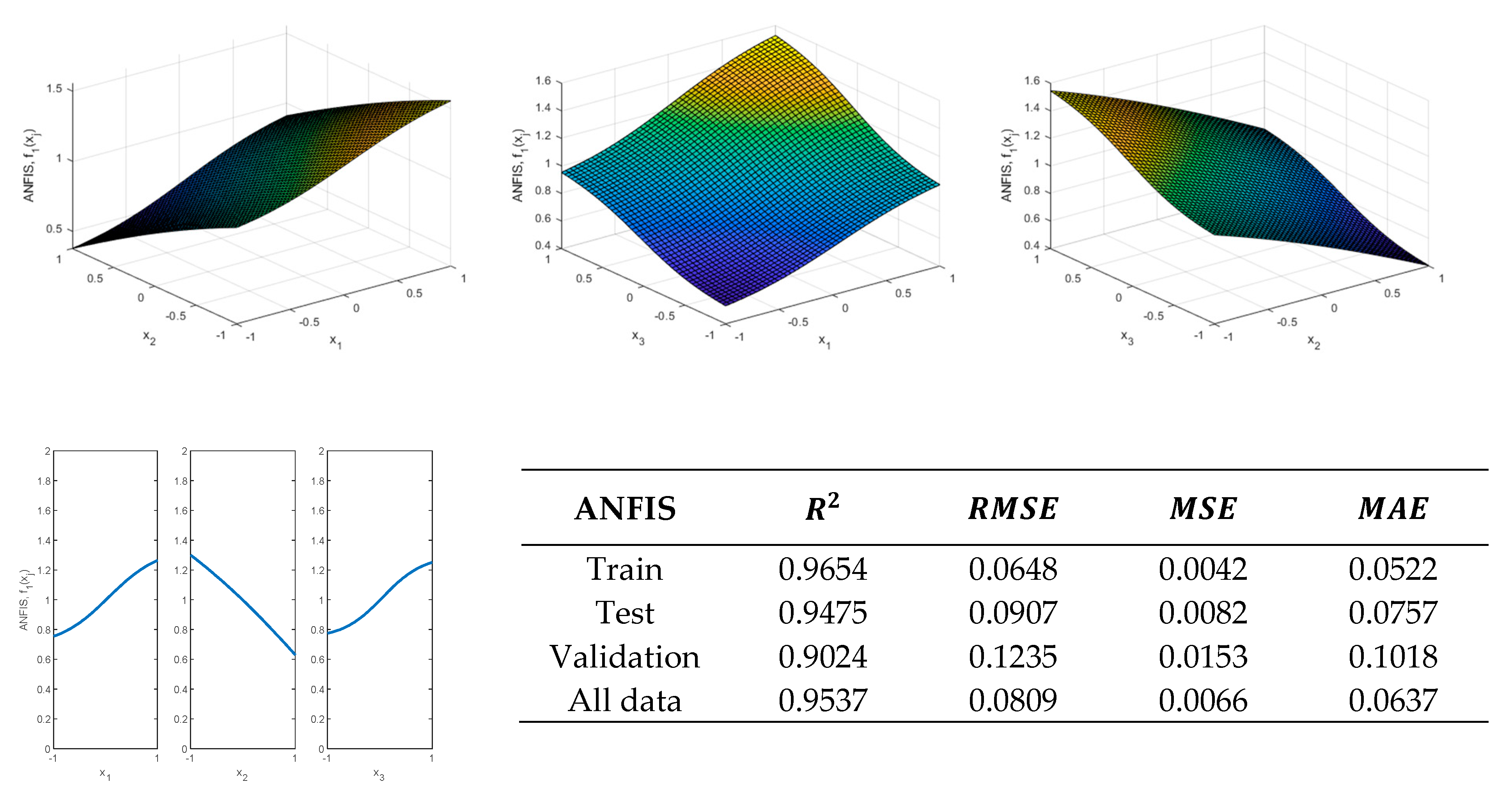
Figure 4 shows the results obtained from the model fitted with the train data. In addition, the results of the validation metrics are shown in
Figure 4. From these results, it is possible to affirm that this model could be applied to analyze the behavior of the response surface shown in
Figure 2a. However, although this regression model could be used to draw some conclusions about the response variable, it presents some limitations because the coefficient of determination when using test data is slightly lower than that obtained with the train data. This can also be observed if the main effects plots obtained with the fitted model and those obtained with the actual function are compared, which are shown in
Figure 4 and
Figure 5, respectively.
Figure 4 and
Figure 6 show the response surfaces obtained with the RSM model when fitting the data from
Table 2 and
Table 3, for types 1 and 2 functions, respectively. The validation metrics employed for measuring the goodness of the fit are mean squared error (
), RMSE and mean absolute error (
). These validation metrics are defined by Equation (3), where
are the actual values and
the estimated values.
On the other hand,
Figure 6 shows the regression results for
function. As can be observed, the regression model cannot adequately predict the behavior of
function. As mentioned earlier, if the evaluation metrics used to assess the goodness of fit (
) provide appropriate values, the RSM model could be used to analyze the behavior of the response variables versus the inputs as well as analyzing the interaction factors. However, this is not the case for
function and therefore, in this case, when using methodologies such as RSM, it would not be possible to trust the model obtained. Therefore, it is necessary to use some other types of methods that allow a better approximation to be obtained from the real behavior of the dependent variable.
As previously mentioned, from the validation metrics shown in
Figure 4 and
Figure 6 it can be affirmed that the RSM model is suitable for modeling a function of type 1 (
) and, therefore, it can be used to analyze the influence of the input variables on the response variables despite the fact that the values obtained in the validation and in the test are lower than those of the training. For example, as can be seen in
Figure 4, increasing the values of variables
and
increases
function and increasing
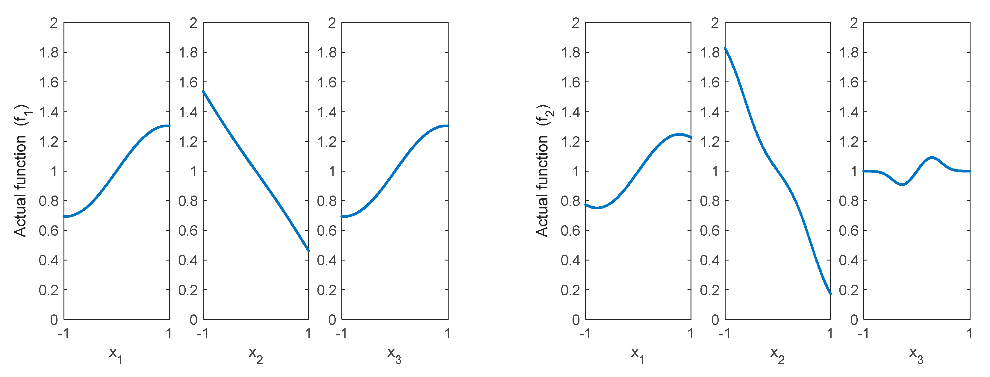
leads to a decrease in the function. If the values obtained with the regression are compared with those that would be obtained with the actual curve, which is shown in
Figure 5, it is shown that in this case the regression provides adequate values and, therefore, it could be used to achieve an approximation to the actual behavior of the function. On the contrary, for
function large discrepancies can be observed in the main effect plots, when comparing the actual results with those obtained from RSM, which are shown in
Figure 5 and
Figure 6, respectively. As can be seen in
Figure 6,
function cannot be properly modeled by a regression using the RSM. Therefore, soft computing techniques will be used to avoid the above-mentioned drawbacks of the RSM models.
4.2. Artificial Neural Network (ANN) Modeling
As shown in the previous section, the RSM model could be used for modeling the behavior of
function. However, in the case of
function, RSM is not able to correctly predict its behavior. Therefore, other types of soft computing-based tools will be used for its modeling. First, a neural network will be trained, using the train data shown in
Table 2 and
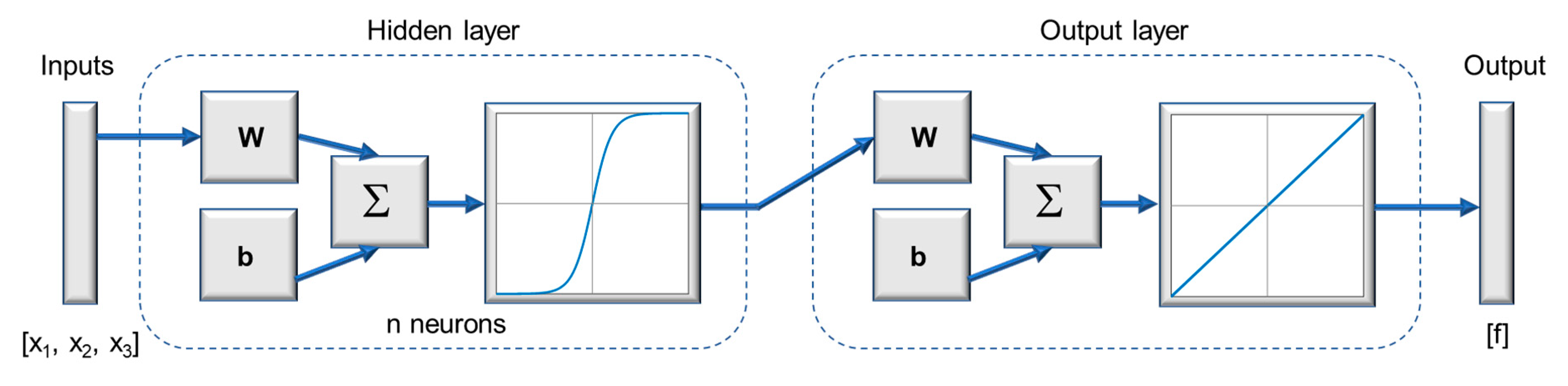
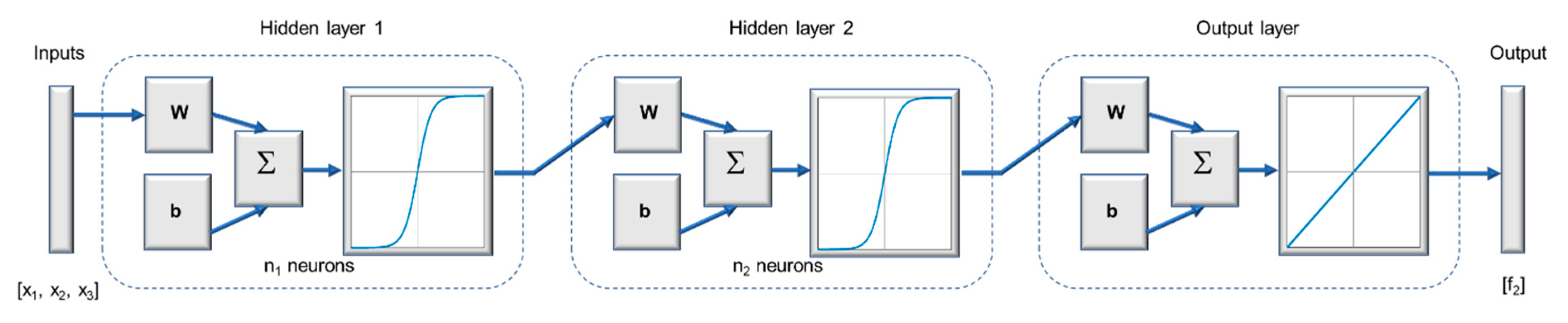
Table 3. The neural network to be used is shown in
Figure 7, where the inputs correspond to the DOE factors
. In this present study the dimension of the input vector will be
since the neural network is to be trained with the 44 points indicated in
Table 2 and
Table 3, for
and
, respectively. The number of neurons in the hidden layer will be varied, starting from
n = 1, as shown in
Figure 7 and the transfer function to be used is a hyperbolic tangent sigmoid transfer function [
64] which is shown in Equation (4). In addition, a Levenberg–Marquardt back-propagation algorithm will be used, using the functions of the Deep Learning Toolbox™ of Matlab
TM2019b [
64]. From the above, a neural network will be used for
and another for
, since due to the variability that exists between the data generated from types 1 and 2 functions it is likely to have a different structure. To obtain the model fitted with the ANN, an iterative process will be carried out for each function that will consist of calculating
neural networks with each ANN structure and, among those ANNs, the one which obtain, first, the lowest MSE in the validation, and secondly the best results in the other validation metrics, will be chosen.
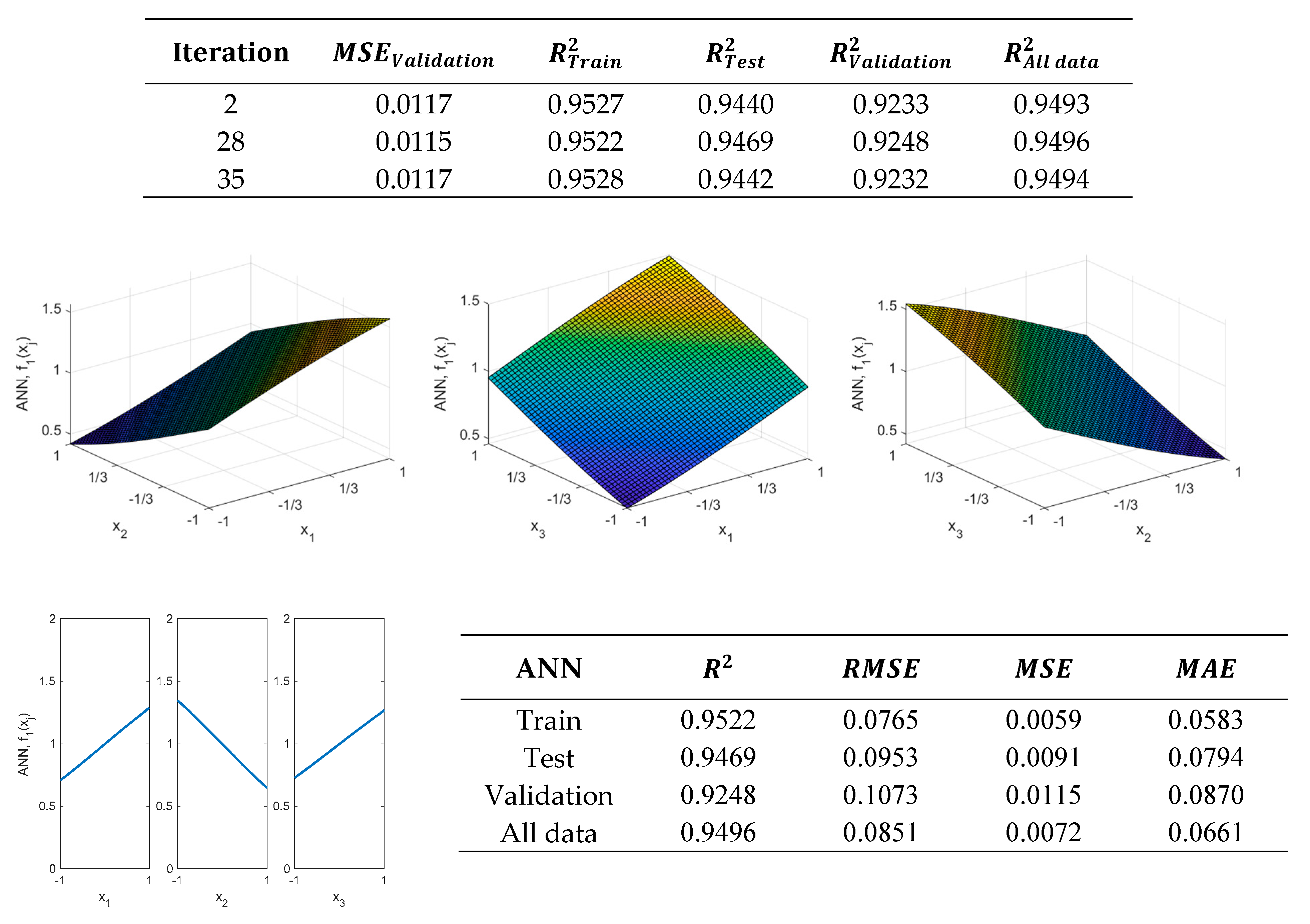
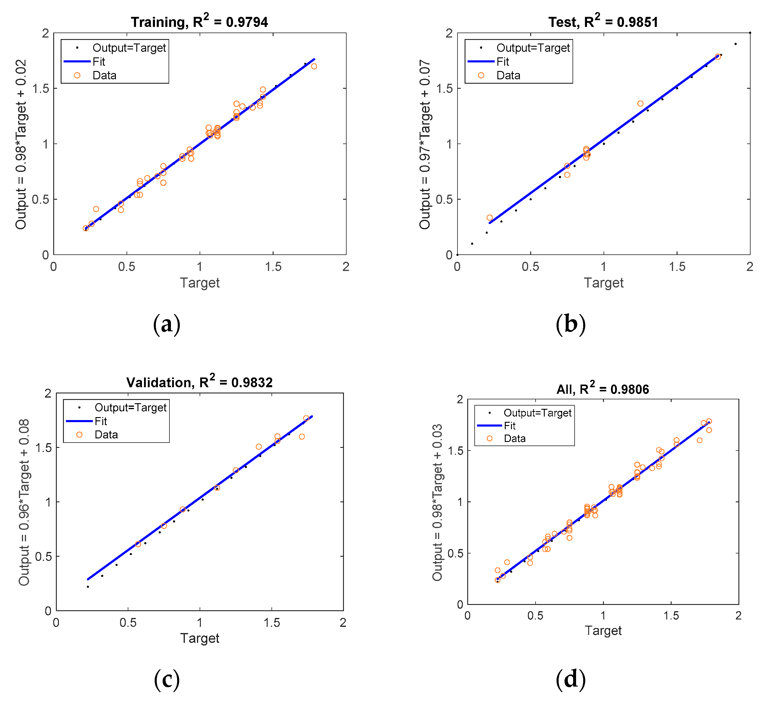
Figure 8 shows the results of the validation metrics shown in Equation (3), obtained using the ANN structure shown in
Figure 7 with
neuron in the hidden layer. This ANN was obtained in the 28th iteration. As can be observed, these values are better than those obtained with the regression model, in the case of the
function, which has been shown in
Figure 4.
Equation (5) shows the results obtained by modeling the
function using an ANN with one neuron in the hidden layer. In this case, the obtained expression is somewhat simpler than that obtained with the RSM and provides slightly better results. Therefore, it could be used to model the response of the
function. If more precision is required, it would be necessary to increase the number of neurons in the hidden layer, but this would lead to more complex expressions to be obtained.
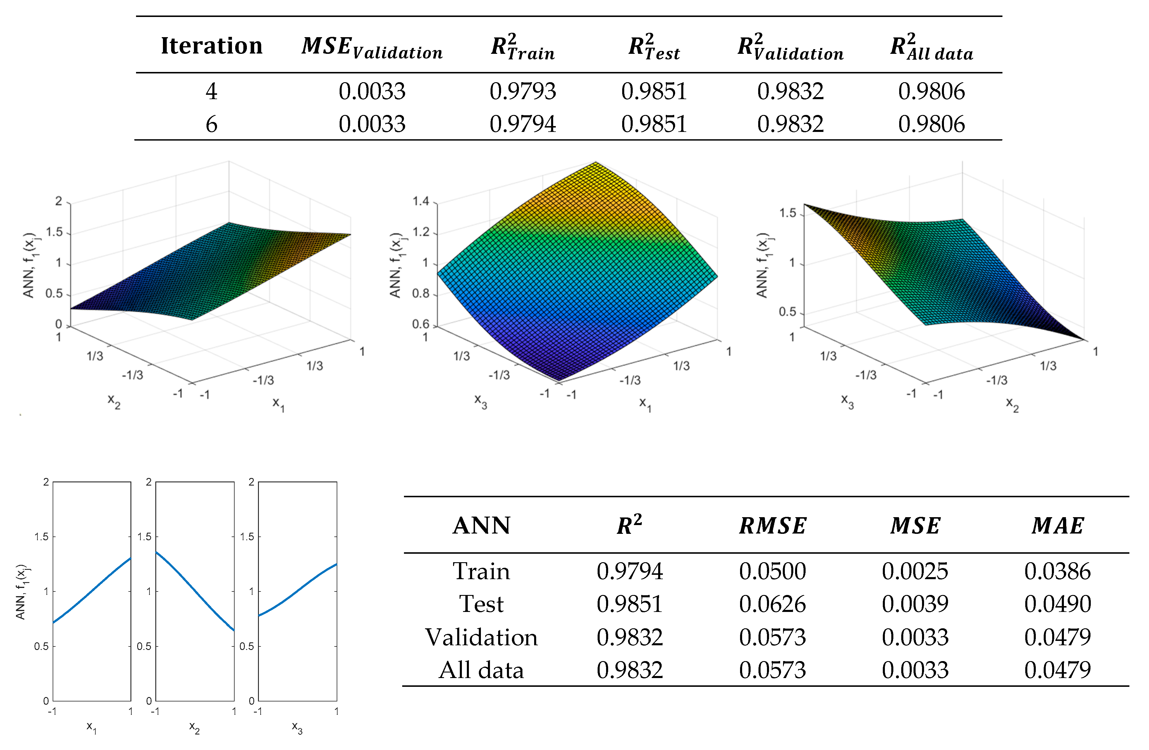
As previously mentioned, if more precision is required, an additional neuron could be added to the hidden layer. Thus, for example, if the hidden layer is made up of two neurons, the results shown in
Figure 9 are obtained, where it is possible to observe that the ANN with two neurons, obtained in the 6th iteration, allows obtaining improved results in the validation metrics.
Moreover, it is possible to increase the number of neurons in the hidden layer. However, the obtained model will be more complex.
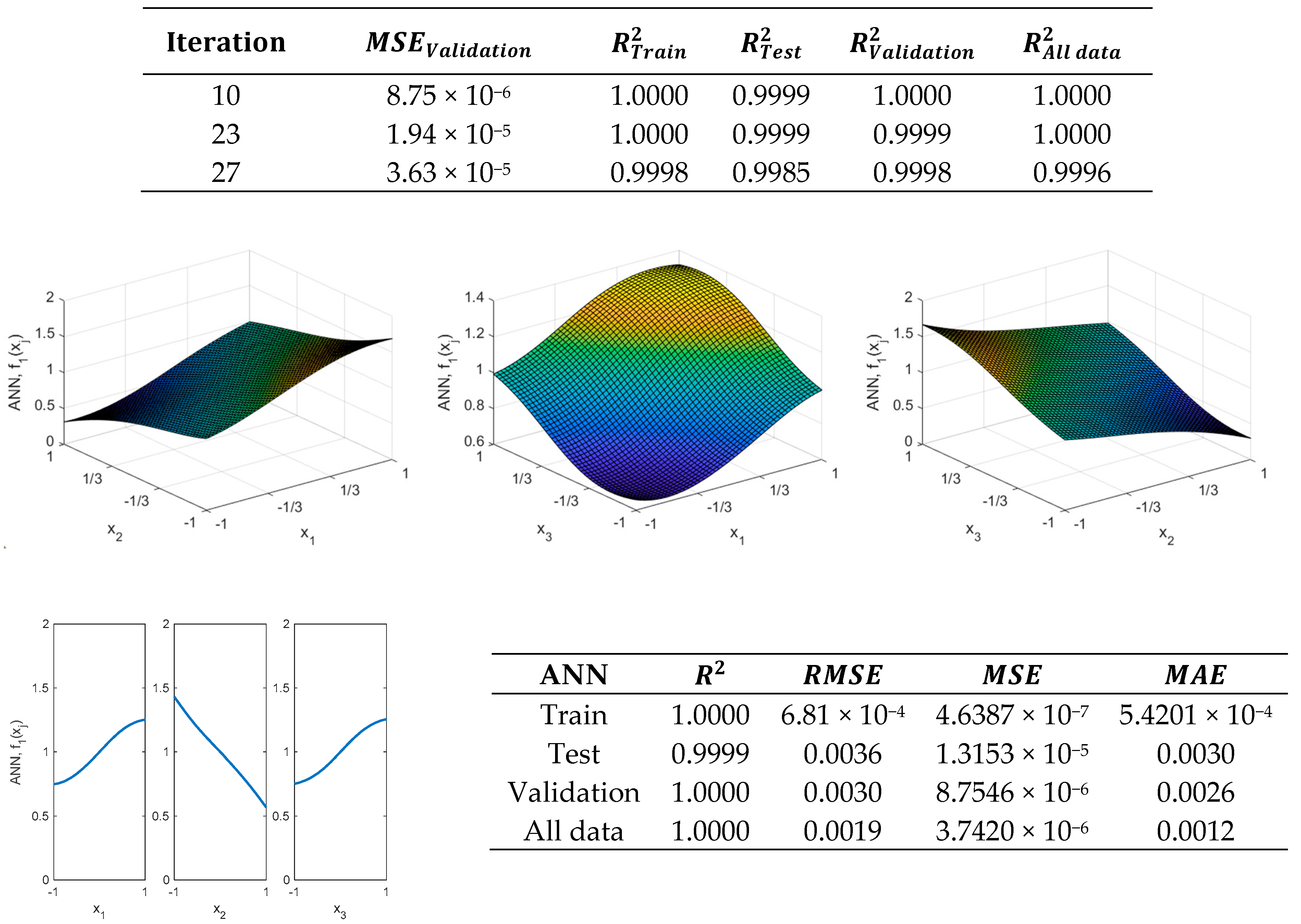
Figure 10 shows results obtained when using the ANN, found in the 10th iteration, which has eight neurons in the hidden layer.
If the
results are compared between the RSM and ANN models, which are shown in
Figure 4 and
Figure 9 (
), i.e.,
, it is observed that
are lower in all cases (−27.22%, −35.66%, −60.99%, −36.33%). A similar result is observed with the
(−27.99%, −45.25%, −58.67%, −39.57%). Moreover,
Figure 11 shows that the coefficients of determination of the regression are higher in all cases (0.98, 0.99, 0.98, 0.98). Regarding the ANN with (
).
Figure 8 shows that the validation metrics obtained with this model are somewhat higher with the train data, but they are lower in the validation, test, and with all data (11.35%, −2.06%, −26.96%, −5.44%). A similar result is obtained with
MAE (8.77%, −11.28%, −24.94%, −4.20%). In any case, since the RSM in this case provides values close to those given by the neural network, in this particular case the RSM model could be used since the values of the coefficient of determination of the regression for the
function are (0.96, 0.93, 0.87, 0.94) in the analyzed cases (train, test, validate, and all data). However, the model with one neuron provides a somewhat improved model (0.95, 0.94, 0.92, 0.95) compared to that obtained with the RSM.
In the case of
function a Levenberg–Marquardt back-propagation algorithm is also used in order to update weights and biases of the ANN by employing the Deep Learning Toolbox™ of Matlab
TM2019b [
64].
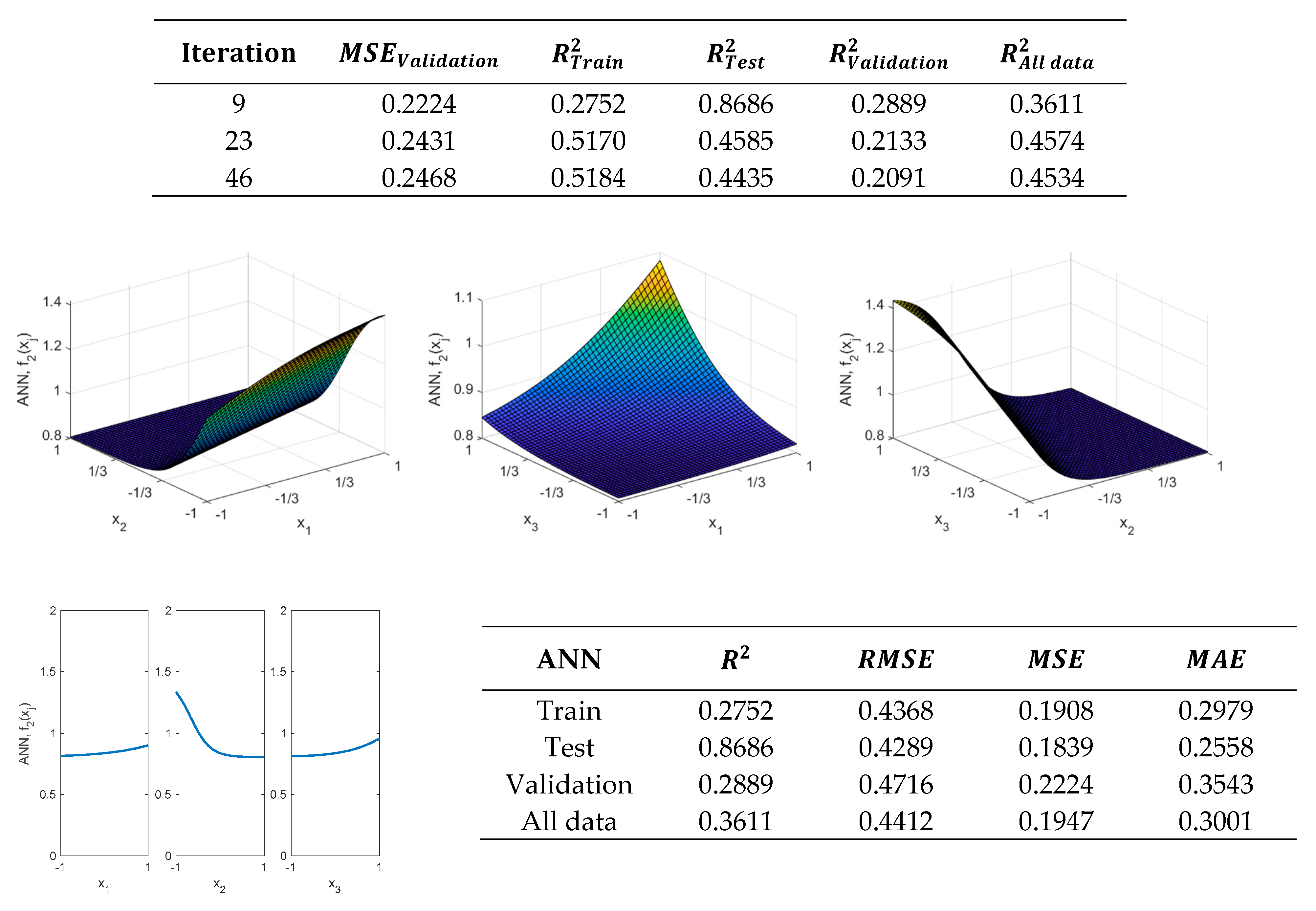
Figure 12 shows results obtained with one neuron in the hidden layer.
As
Figure 12 shows, regression results do not improve with a neuron. Therefore, the number of neurons in the hidden layer will be increased until better results are obtained. For example, with two neurons in the hidden layer, an increase in the coefficient
as well as a decrease in both RMSE and MAE are attained.
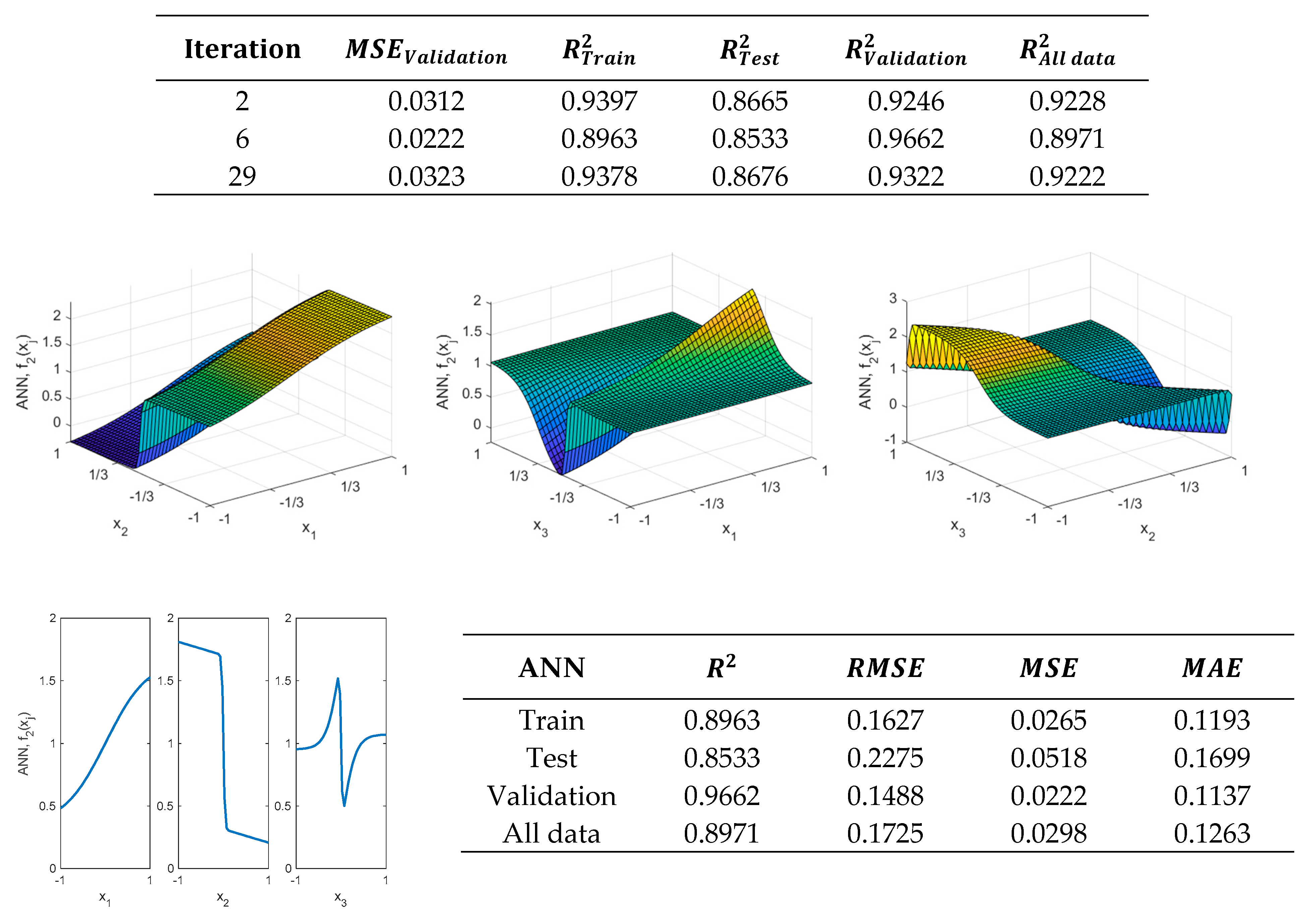
Figure 13 shows that the validation metrics significantly improve, compared to those obtained with one neuron in the hidden layer when using the ANN obtained in the 6th iteration.
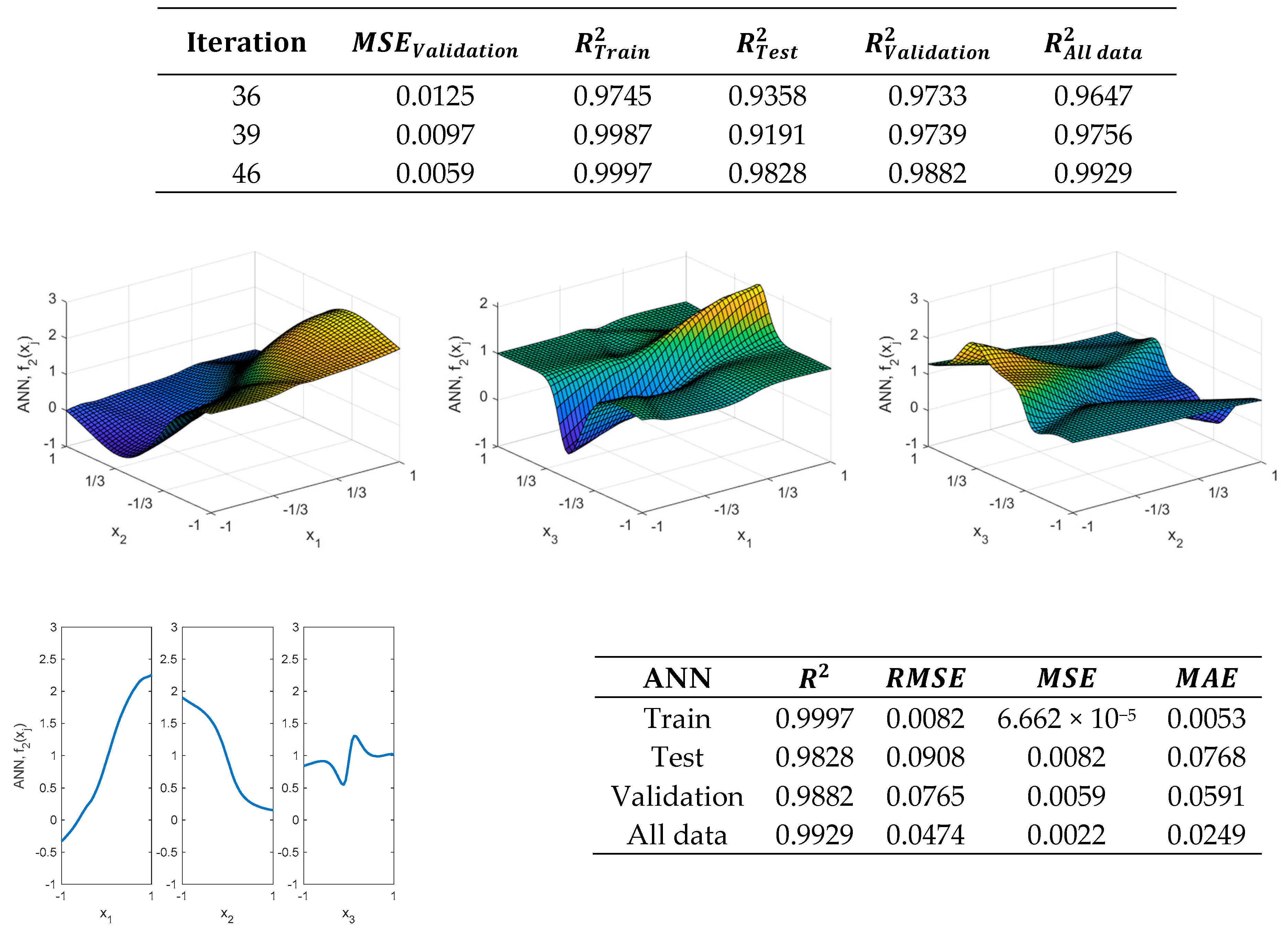
Figure 14 shows that the R-squared result is approximately 1 in the train data with the neural network, obtained in the 48th iteration, which has 8 neurons in the hidden layer. In addition, the results of the validation metrics are also improved for both test and validation data. However, as can be observed by comparing
Figure 2 and
Figure 14, this neural network is neither able to reproduce the actual shape of the
function. Furthermore, a two-layer ANN could also be used for modeling
, as
Figure 15 shows.
Although the transfer functions of this ANN are not required to be the same, those shown in Equation (4) will be used. In addition, a Levenberg–Marquardt back-propagation algorithm will be used by employing the Deep Learning Toolbox™ of Matlab
TM2019b [
64].
As
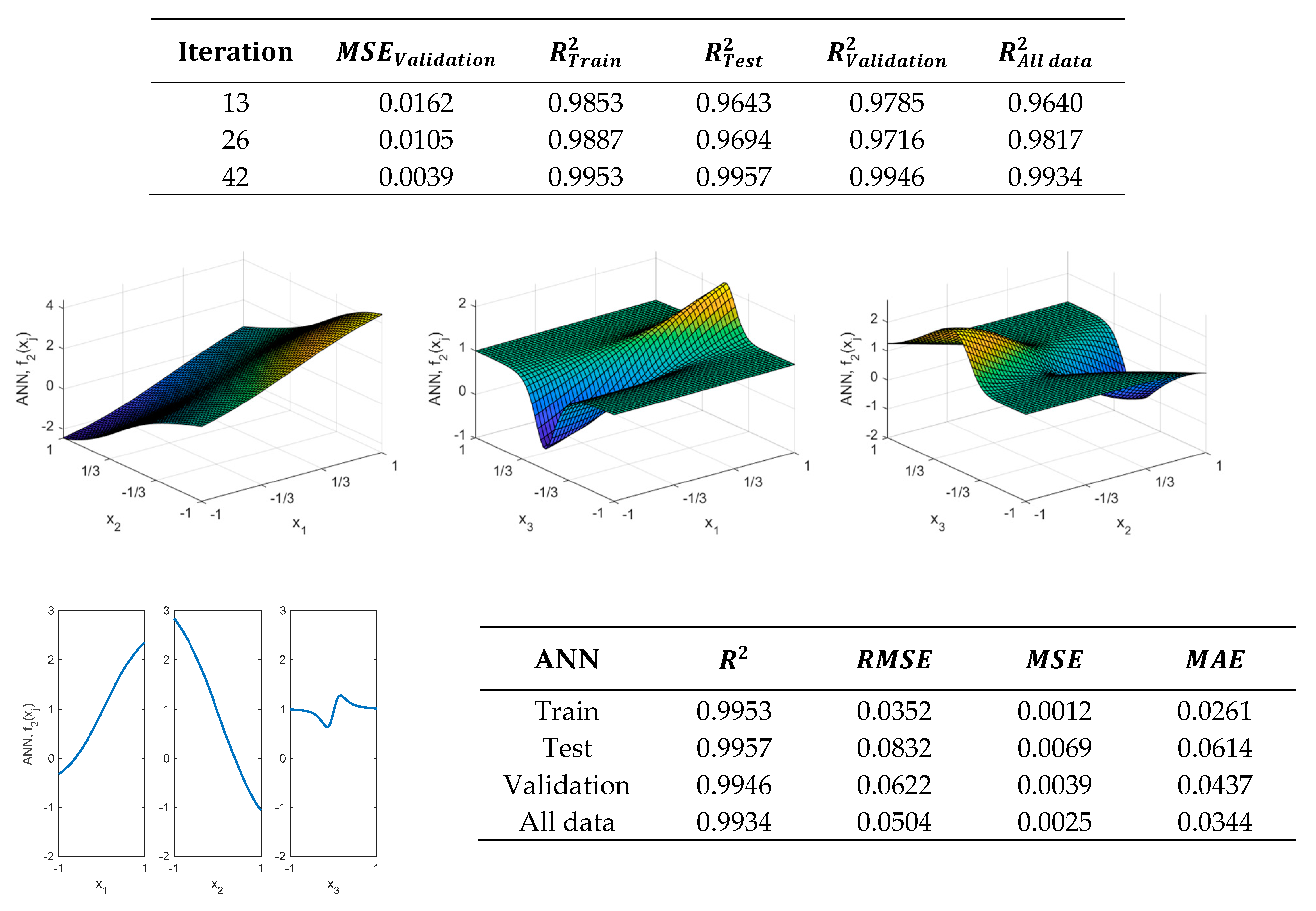
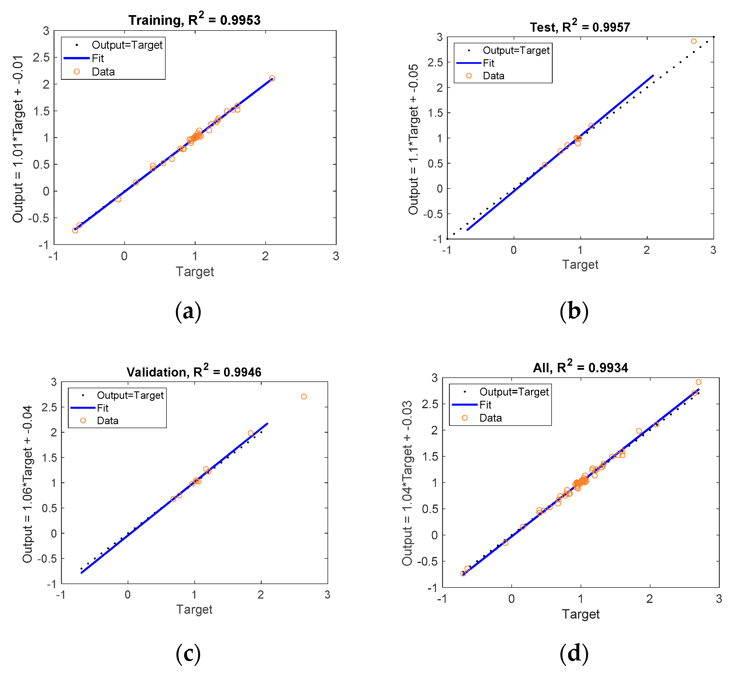
Figure 16 shows, by using two hidden layers a significant improvement is attained in the validation metrics shown by Equation (3).
Figure 17 shows that the
, which is obtained after the 42nd iteration, can provide higher values of the coefficient of determination. Although the complexity of the model is higher than that of RSM, the RSM model does not provide adequate values for modeling the
function.
On the other hand, the neural network, despite providing values closer to the behavior of
, requires many parameters for this. In any case, the neural network can model the behavior of the
function much better than the RSM and can provide much better values in the validation metrics than those obtained with the regression model. However, this ANN is neither able to fully reproduce the actual shape of the
function, as can be observed when comparing the response surfaces obtained in
Figure 2 and
Figure 16.
4.3. Adaptive Neuro-Fuzzy Inference System (ANFIS) Modeling
In this present study, two strategies are shown to model the behavior of types 1 and 2 functions using an ANFIS. First, a modeling based on the Matlab
TM2019b functions is used, which is shown in this current
Section 4.3, and secondly, in
Section 4.4, a new methodology is proposed.
Figure 18 shows the two strategies that will be considered.
With regard to the first strategy, the “genfis” function of Matlab
TM2019b [
66] will be used to obtain a zero-order Sugeno FIS and then an ANFIS will be used to tune the parameters of the membership functions. Secondly, another strategy is proposed in this study which consists of using an iterative process to obtain the FIS from the DOE and then using an ANFIS for tuning the constants of the membership functions. As will be shown in
Section 4.4, with this proposed methodology, it is possible to obtain improved results in both the validation metrics and in the modeling of the actual shape of the function.
As was previously mentioned, a zero-order Sugeno FIS is employed by using the Fuzzy Logic Toolbox™ of Matlab
TM2019b [
66], because the de-fuzzification process for a Sugeno system is computationally more efficient compared to that of a Mamdani system [
66,
67,
68]. However, it should be mentioned that Mamdani systems are more intuitive and the rules are easier to understand, making them more suitable for expert systems, developed from human knowledge [
66,
67,
68]. Both types of FIS could have been used.
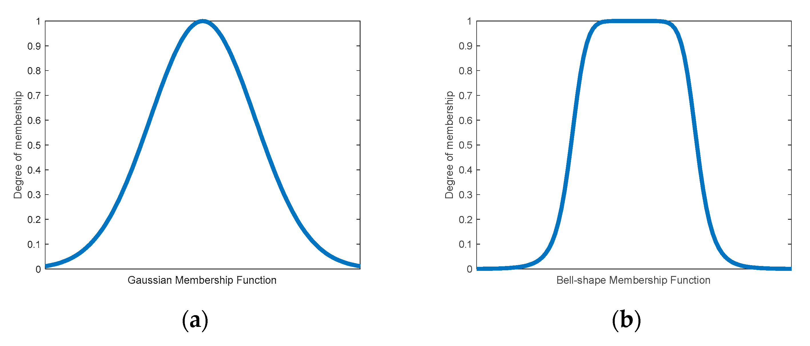
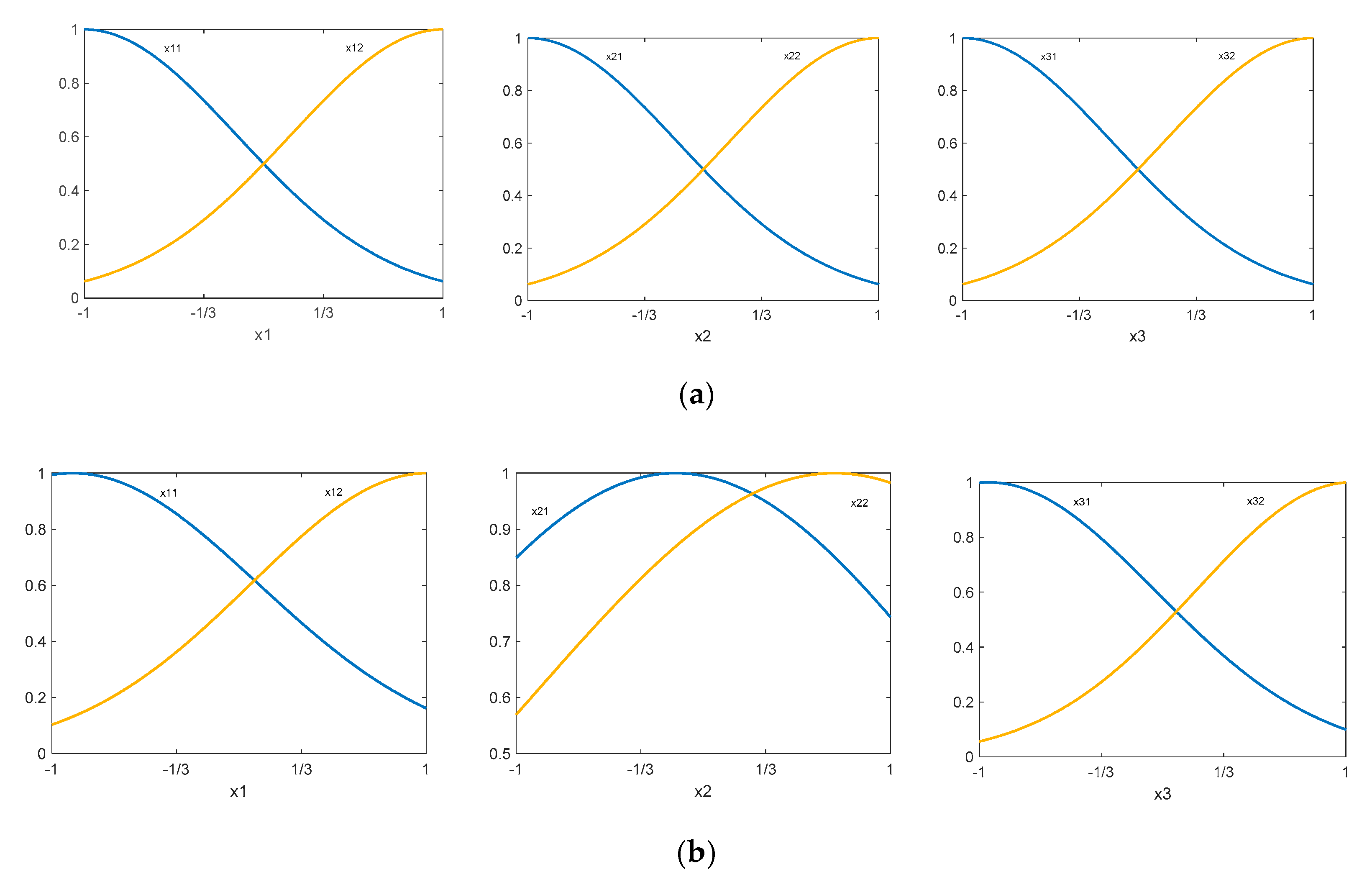
Figure 19 shows two membership function that could be used for fuzzification of the inputs. The membership functions to be used in this study are of the Gaussian type. However, some other types of membership functions such as triangular or bell-shape could have been used.
As previously mentioned, the first strategy is to use the Matlab™2019b “genfis” function [
66] to obtain a zero-order Sugeno FIS from the input data. It should be mentioned that it would have been possible to start from the inputs and the outputs and to use some algorithm of the type pattern search or genetic algorithm in order to find a set of rules that model the behavior of the response variables. However, this has not been done in this present study. Furthermore, the membership functions for fuzzification of the independent variables are Gaussian as shown in Equation (6).
The aggregation method is the sum of fuzzy sets, and the aggregated output is obtained from the weighted average of all output rules. For the
rule, the implication method is obtained from Equation (7), where product implication method is used in Sugeno systems [
66] and Equation (8) shows the final output of the Sugeno system.
The created FIS will have a set of
rules of the form:
From the above, a zero-order Sugeno FIS [
2,
3,
66] is selected with Gaussian membership functions.
Figure 20 shows the Gaussian membership functions for the zero-order Sugeno FIS employed for modeling
, before and after using the ANFIS. It should be mentioned that a greater number of membership functions could have been used for modeling
, but two membership functions for each of the variables was enough. Therefore, 8 rules are generated for the zero-order Sugeno FIS. To train the fuzzy system an ANFIS employing the Fuzzy Logic Toolbox of Matlab
TM along with a back-propagation algorithm has been used [
66]. This training process adjusts the membership function parameters of a FIS such that the system models the input/output data.
Table 6 shows the values of the Gaussian membership functions, where
and
are the parameters of the Gaussian function shown by Equation (6) and
Table 7 shows the rules obtained after the ANFIS.
Figure 21 shows the results obtained by using a zero-order Sugeno FIS for modeling
using two Gaussian membership functions for each of the inputs after 100 epochs.
Regarding
function, first a zero-order Sugeno was generated. From this, the membership functions before and after using an ANFIS are shown in
Figure 22.
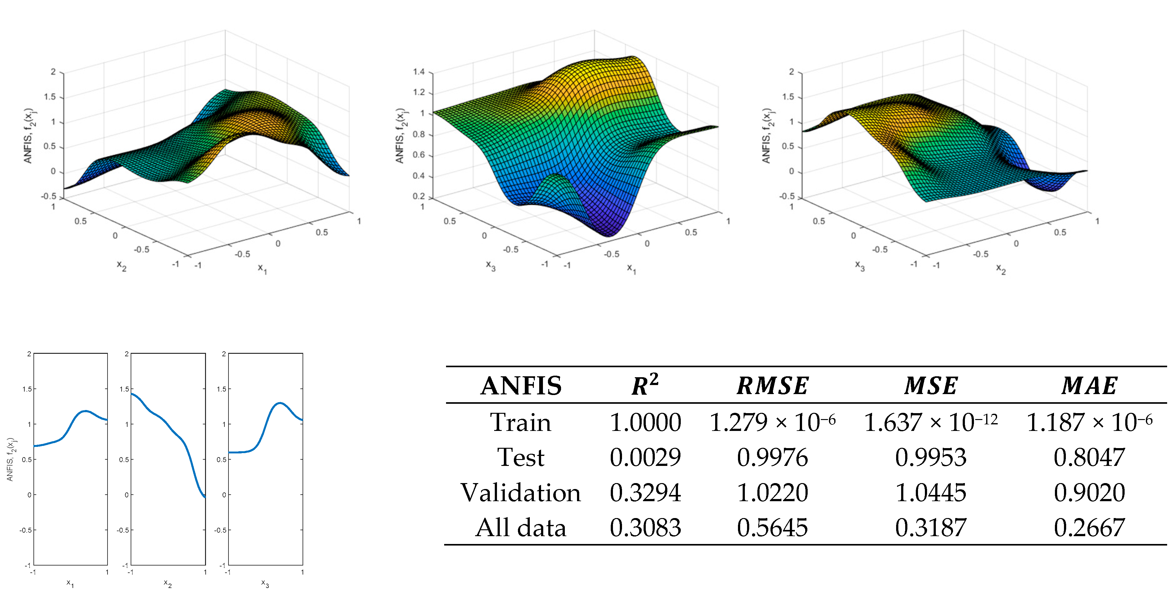
Figure 23 shows the results obtained by modeling the function using the membership functions shown in
Figure 22a and then using an ANFIS. In this case, it is shown in
Figure 23 that after 500 epochs it has not been possible to adequately model the function
.
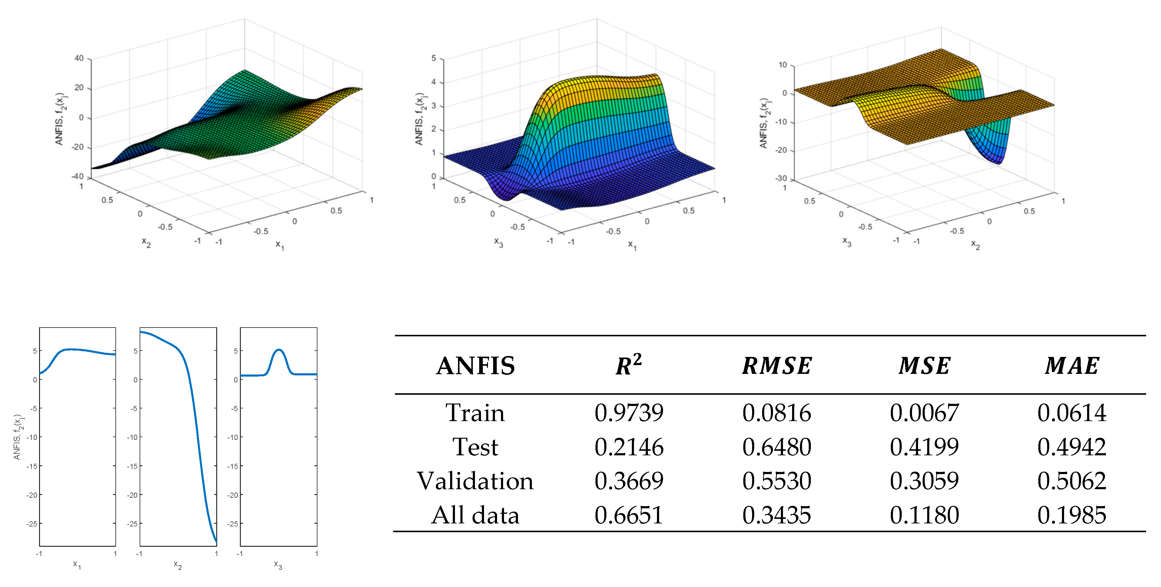
If the membership functions are increased to three, a satisfactory result is not obtained either, as
Figure 24 shows.
A similar behavior is obtained using four membership functions. Although the values of the validation metrics obtained with the train data are adequate, this is not the case with the validation and test data, as
Figure 25 shows. Therefore, a new procedure for obtaining an ANFIS is to be proposed in the next section that avoids these drawbacks. As will be shown in the next section, the accuracy of the thus obtained model is higher than that obtained with the previous method.
4.4. Proposal of a Method for Obtaining an Adaptive Neuro-Fuzzy Inference System
One of the advantages that FIS have over other computing tools is that it is possible to take advantage of the user experience to generate them. In this section, the FIS is generated directly from the train data of the DOE. Therefore, from data shown in
Table 2 and
Table 3, it will be possible to directly obtain the set of rules that make up a zero-order Sugeno FIS. Then an iterative process will be followed, and the FIS parameters will be tuned using an ANFIS, according to the procedure shown below. Once the adjusted models have been developed, the results obtained will be analyzed in a similar way to that used for the case of RSM and ANN.
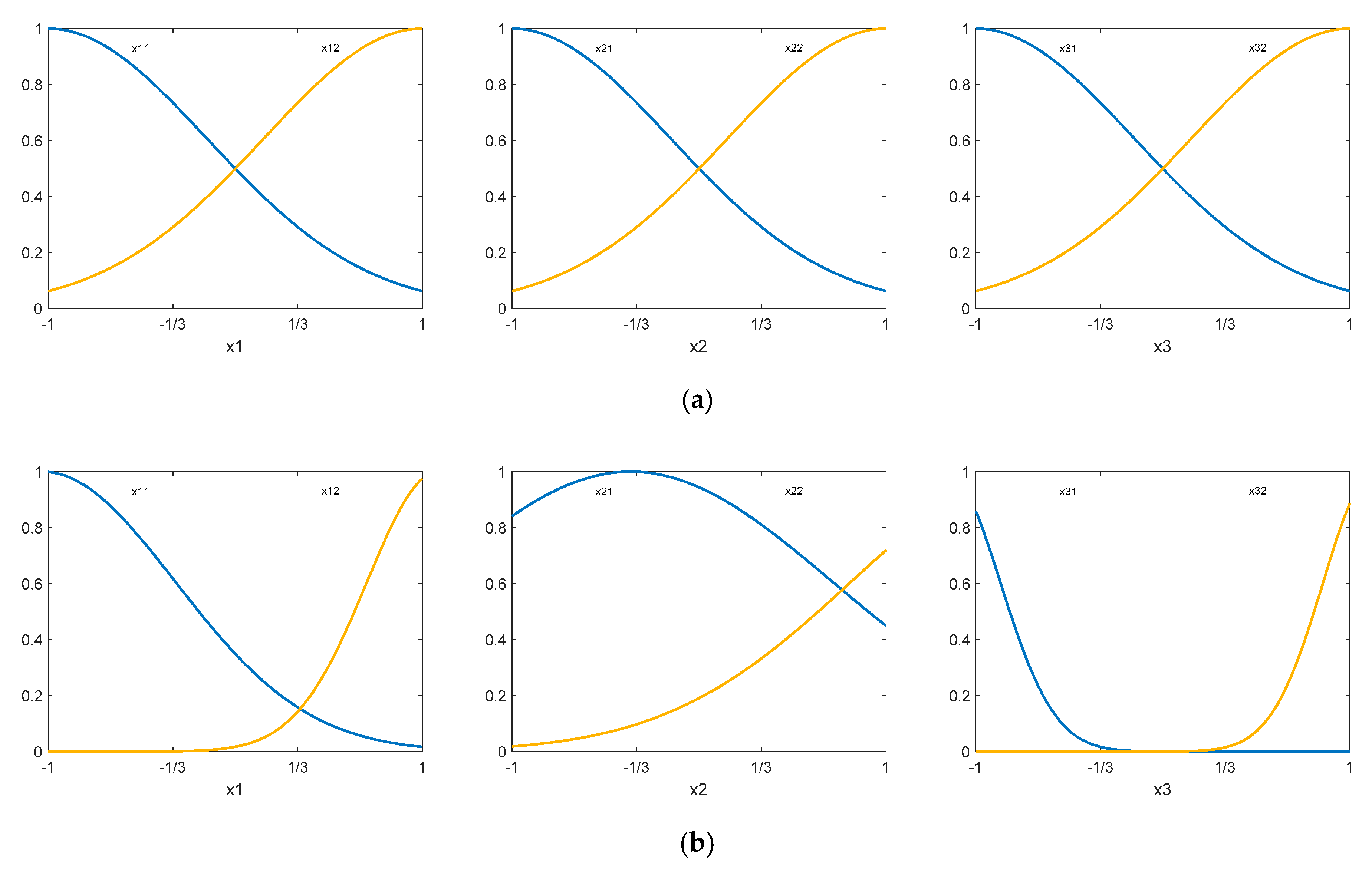
The proposed methodology begins by selecting membership functions of the Gaussian type, such as those shown in Equation (9). The standard deviation values of the membership functions are obtained from Equation (10) and the corresponding levels of the DOE will be used for the mean values of the membership functions, as shown in Equation (11). Since the DOE has four levels for the input variables, as shown in
Table 1, four Gaussian functions will be employed, as shown in Equations (9)–(11). From this, a zero-order Sugeno FIS will be developed from the DOE and then it will be tuned by using an iterative process and an ANFIS, i.e.:
where the levels of the variables
are obtained from the DOE shown in
Table 1, where
,
,
and
can be increased with respect to the previous one in order to introduce an imbalance in the form of the membership functions, if necessary, or they can be the same. Based on the above, different initial FIS can be obtained by varying the values of
and
. As was previously mentioned, a zero-order Sugeno FIS will be used in this study. The proposed procedure is based on adjusting the parameters of the membership functions using an iterative process combined with an ANFIS.
To summarize the proposed methodology, the algorithm that has been programmed to obtain the results shown in this current section is as follows:
- (1)
Select the range of variation of and , i.e., and
- (2)
Select the increment for variation of and
- (3)
Select the maximum number of Epochs as well as the initial value of and , where is the desired level for and is the desired level for .
- (4)
Determine the strategy to calculate the values of the membership functions constants.
(4.1) A full iteration can be followed to look for and .
To reduce the running time, two strategies may be considered (either 4.2. or 4.3).
(4.2) It is assumed that and (That is a double iteration is obtained).
(4.3) Using a constant for all the membership functions and then iterate to obtain (That is: assume a value for . For example, and then iterate to obtain ) (That is a triple iteration is obtained).
Then, the algorithm continues as follows:
(4.1a) Iterate to obtain
and
. (As shown in Algorithms 1, if exit
n inputs, then
n iterations would be obtained).
| Algorithms 1. Iterate to obtain and .(Case of n inputs) |
|
| |
| |
| |
| |
| |
| Obtain a zero-order Sugeno FIS, |
| Tune using an ANFIS, that is: |
| For Epochs = 1:: |
| |
| Evaluate using |
| |
| Find min{ to obtain min{ |
| |
| Evaluate using |
| Evaluate using |
| |
| |
| Store calculated FIS, min{ , and |
| Exit of the iteration loop |
| Else |
| Store min{ , and |
| |
| |
| |
| |
| |
| |
|
(4.1b) Iterate to obtain
and
. (The present study considers three inputs variables. As shown in Algorithms 2, if a full iteration is carried out, then six iterations would be obtained).
| Algorithms 2. Iterate to obtain and .(Case of 3 inputs) |
|
| |
| |
| |
| |
| |
| Obtain a zero-order Sugeno FIS, |
| Tune using an ANFIS, that is: |
| For Epochs = 1:: |
| |
| Evaluate using |
| |
| Find min{ to obtain min{ |
| |
| Evaluate using |
| Evaluate using |
| |
| |
| Store calculated FIS, min{ , and |
| Exit of the iteration loop |
| Else |
| Store min{ , and |
| |
| |
| |
| |
| |
|
(4.2) Algorithms 3 shows the procedure to obtain
and
.
| Algorithms 3. Assumed and . |
|
| |
| Obtain a zero-order Sugeno FIS, |
| Tune using an ANFIS, that is: |
| For Epochs = 1:: |
| |
| Evaluate using |
| |
| Find min{ to obtain min{ |
| |
| Evaluate using |
| Evaluate using |
| |
| |
| Store calculated FIS, min{ , and |
| Exit of the iteration loop |
| Else |
| Store min{ , and |
| |
| |
|
(4.3) Algorithms 4 shows the procedure to obtain
, when a value is assumed for
(For example,
).
| Algorithms 4. Iterate to obtain (assumed for ) |
|
| |
| |
| Obtain a zero-order Sugeno FIS, |
| Tune using an ANFIS, that is: |
| For Epochs = 1:: |
| |
| Evaluate using |
| |
| Find min{ to obtain min{ |
| |
| Evaluate using |
| Evaluate using |
| |
| |
| Store calculated FIS,min{ , and |
| Exit of the iteration loop |
| Else |
| Store calculated FIS as well as Epochs,, and |
| |
| |
| |
|
- (5)
Among the results obtained, the one that optimizes the value of .and at the same time meets the condition will be selected.
- (6)
Once the iterations are finished, will be obtained. Then both the validation metrics and the response surface could be obtained by using the tuned FIS.
In this present study, the procedure consisting of obtaining
and
will be followed. Once the optimal values (
and
) have been found, in the first case, or
,
and
, in the second case, the ANFIS, which optimizes the value of
, is obtained directly. As previously mentioned, other alternatives will be possible for obtaining
and
, i.e., iterating with the full set of constants. However, they may require higher running time when
and
are increased. If
and
are set to 1, then a full iteration is carried out. Therefore, the results shown below have been obtained with the strategy of iterating to find (
and
), i.e., look for the values of
and
that lead to a lower
(MSE value obtained with the validation data). If all simulation data are collected, then several solutions could be obtained and, in that case, the value that minimizes the
.will be selected. If there exist several solutions, then the values that minimize the R
2-coeffients obtained with the train, validation, and test data in that order, will be chosen. According to the described procedure, an ANFIS is used together with a back-propagation algorithm to tune the values of the membership functions. Each of the thus obtained FIS are tuned using an ANFIS by employing the functions of the Fuzzy Logic Toolbox of Matlab
TM [
66].
Table 8 and
Figure 26 show the programming results for
function. As indicated, a double iteration is performed to find
and
and at the same time an ANFIS is employed to tune the FIS parameters obtained with each value of
and
.
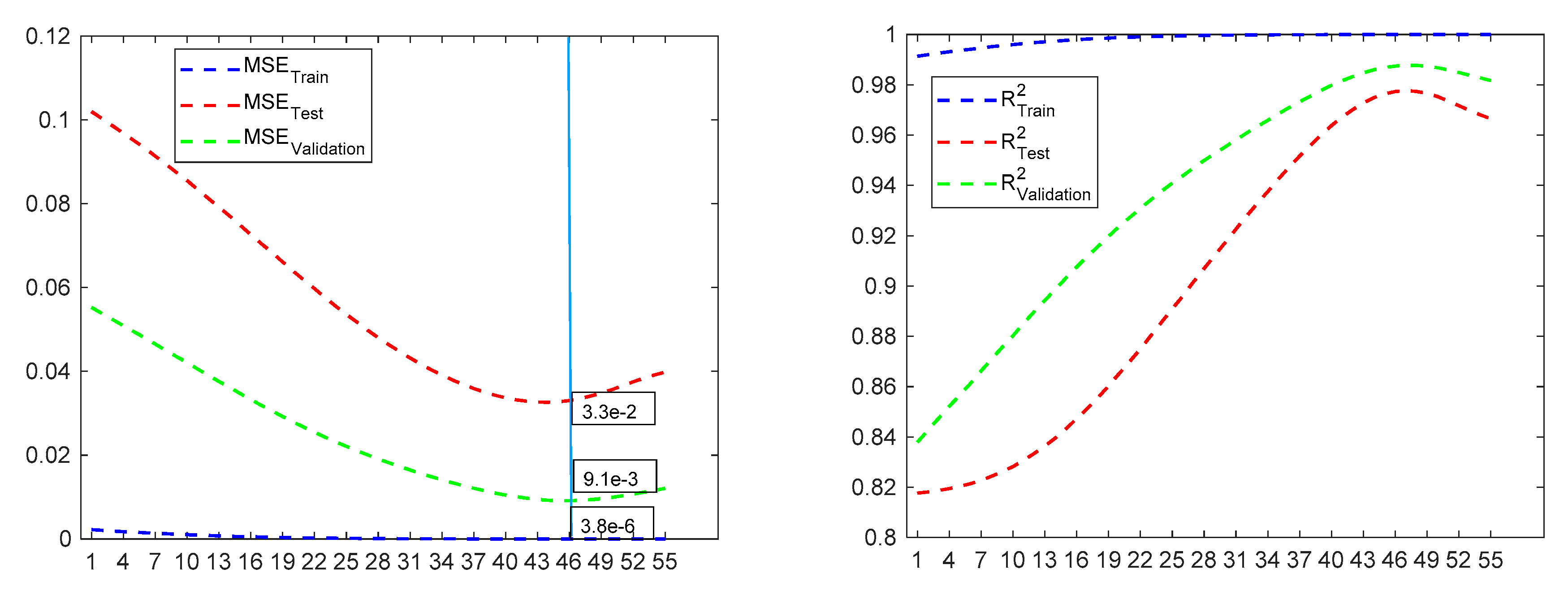
Thereafter, the number of epochs will be increased in the ANFIS for tuning the FIS, the number of epochs that optimizes will be selected and at the same time verifies that and that the maximum number of epochs is not reached. This will lead to the optimal of to be obtained and, subsequently, the obtained ANFIS will be evaluated both in the test and in the train data and finally in all the data.
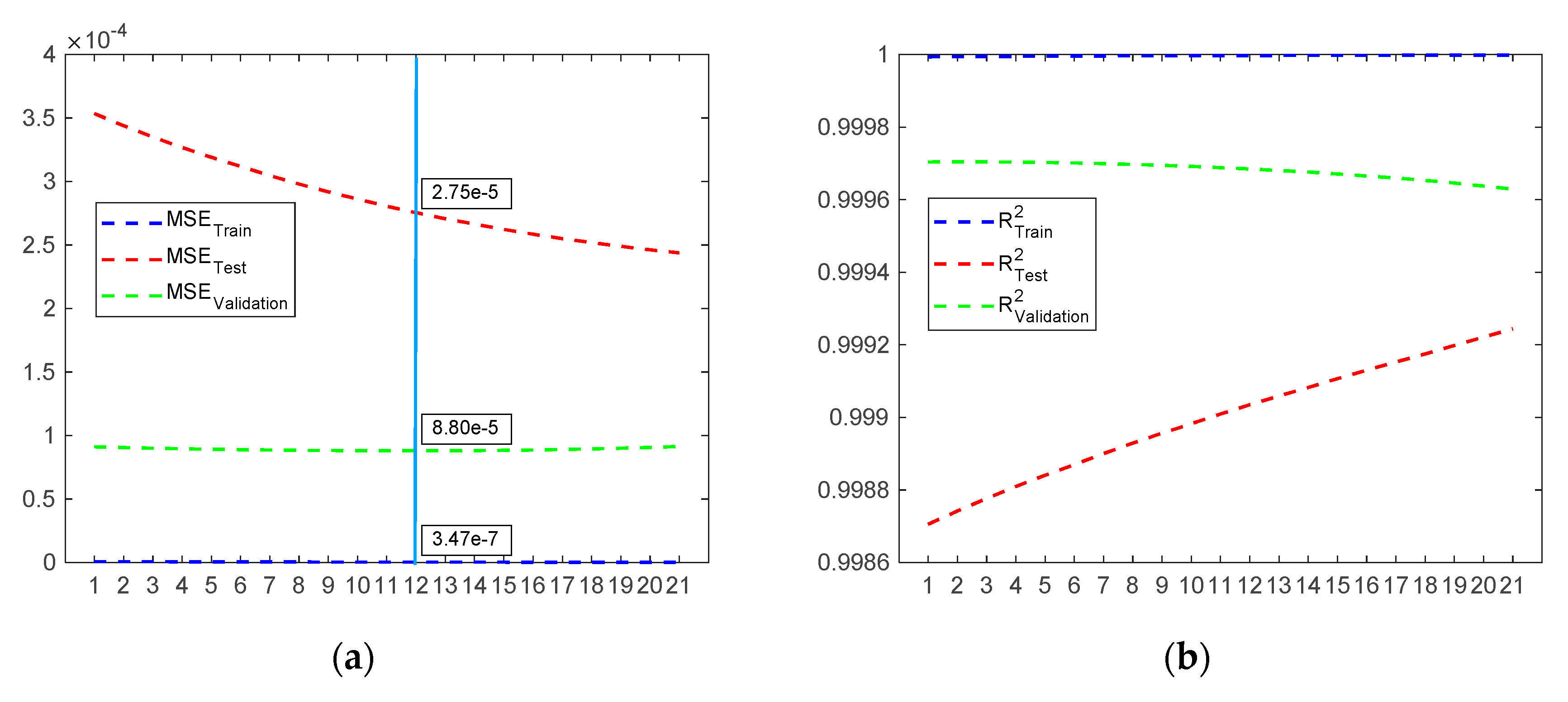
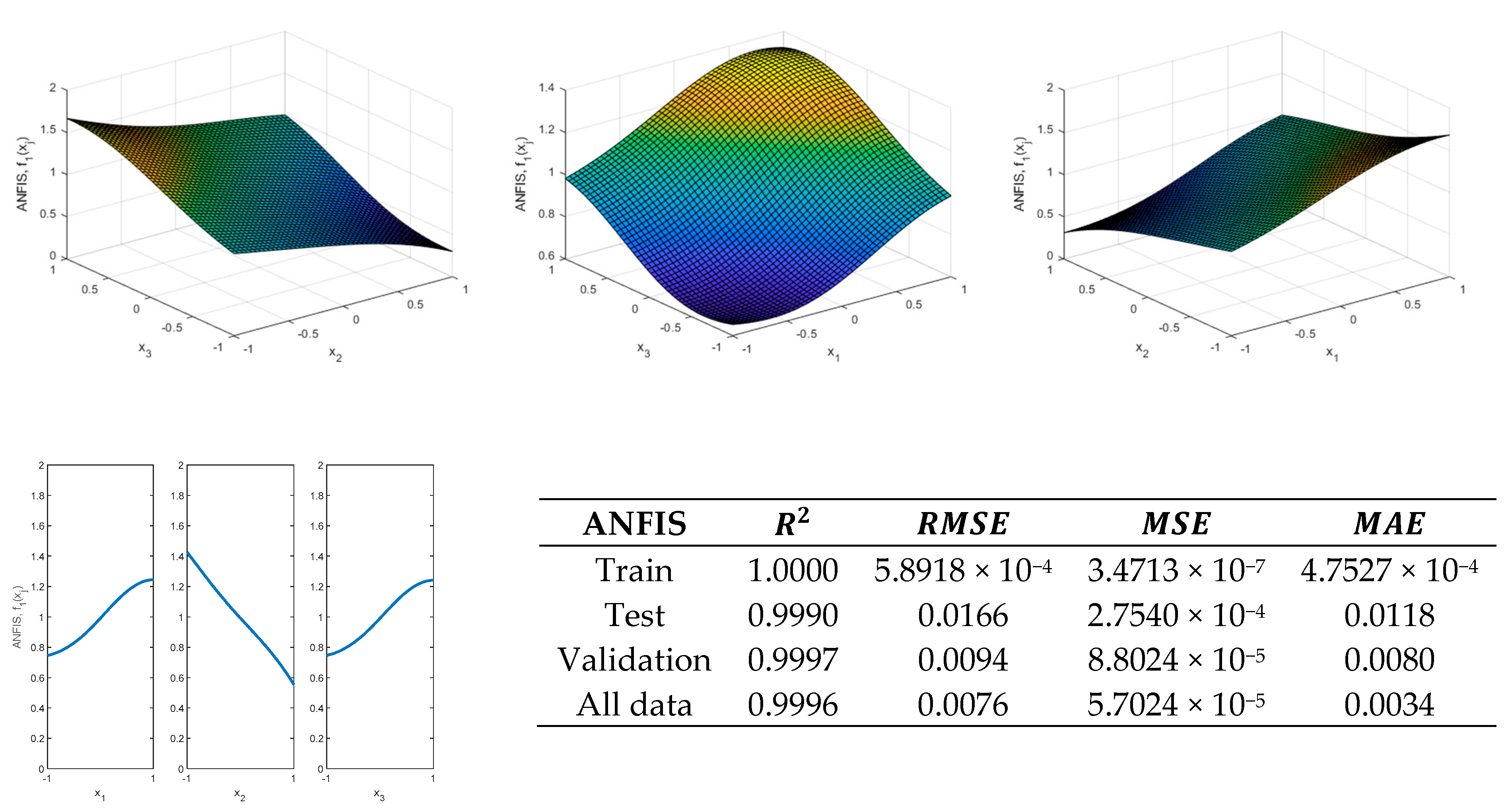
Figure 27 and
Figure 28 show the results obtained with the ANFIS generated from the aforementioned methodology. As can be observed, the proposed method is able to find an approximation with high accuracy. The ANFIS thus obtained which led to better results was the one with
and
and after 10 epochs with the ANFIS.
As can be observed, the ANFIS obtained with the proposed methodology can provide better values of the validation metrics than those obtained with both the RSM model and with the ANN that has 1 and 2 neurons in the hidden layer and the obtained results are similar to those obtained with the ANN that has 8 neurons in the hidden layer, when modeling the behavior of
. However, it should be noted that adding more neurons to the ANN can cause irregularities in the response surface to be obtained. As shown, the FIS obtained through the proposed methodology can provide accurate results that could be used to model the response of type 1 functions (
). As will be seen below with the methodology proposed in this present section, it is also possible to obtain satisfactory results, in the case of type 2 functions (
), opposite to that obtained in the previous section, as is shown in
Figure 23,
Figure 24 and
Figure 25.
The results shown in
Table 9 and
Figure 29 have been obtained with the strategy of iterating to find (
and
) in the case of function
, i.e., look for the values of
and
that lead to a lower
. As with
, a double iteration is carried out to find
and
and at the same time an ANFIS is employed to tune the FIS parameters obtained with each value of
and
. The number of epochs that optimizes
will be selected and at the same time verifies that
and that the maximum number of epochs is not reached. Result obtained are
and
for the initial FIS and the tuned FIS is achieved after 46 epochs using an ANFIS that tune the initial parameters of the FIS adjusted with the previously mentioned
and
.
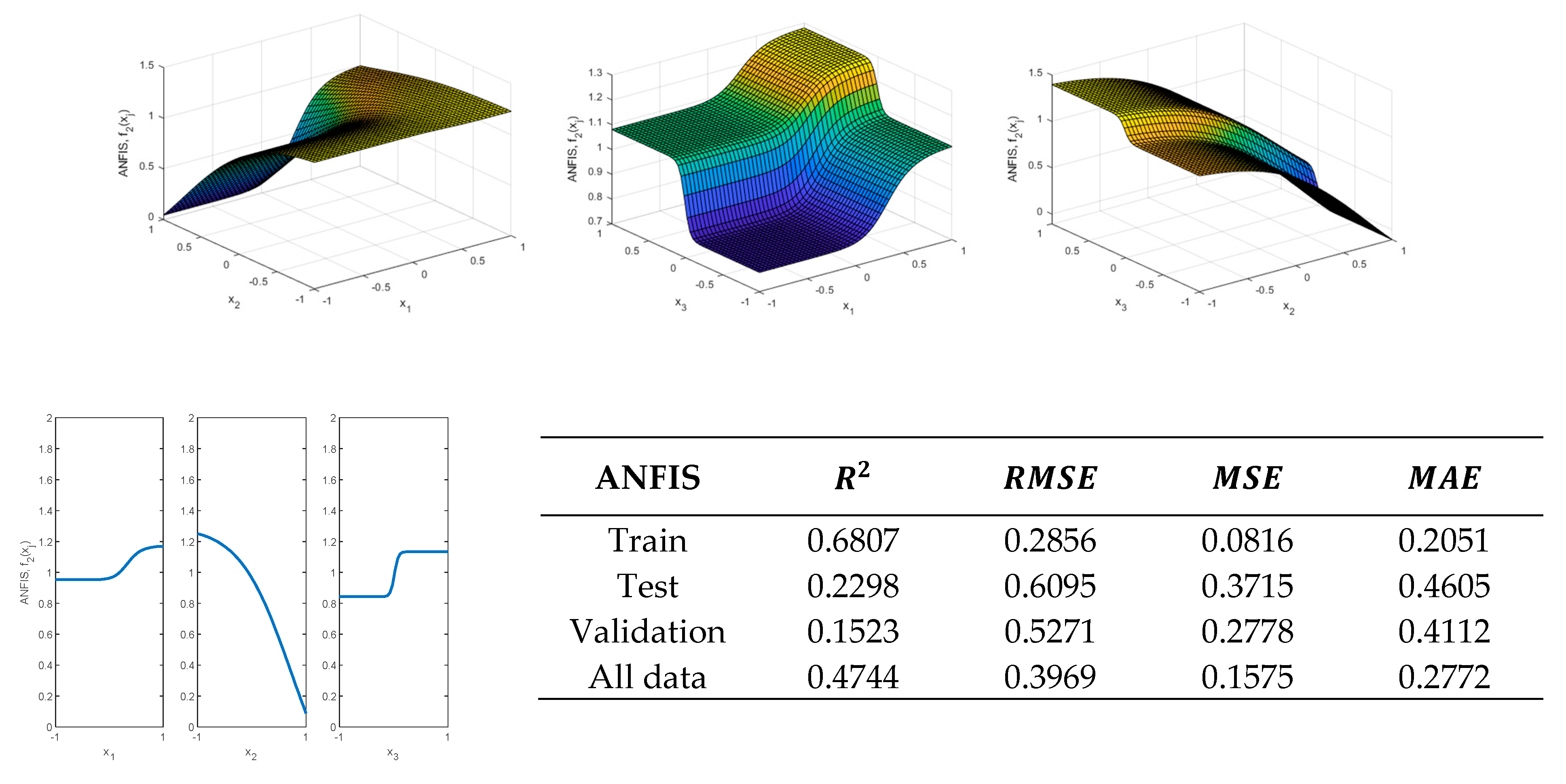
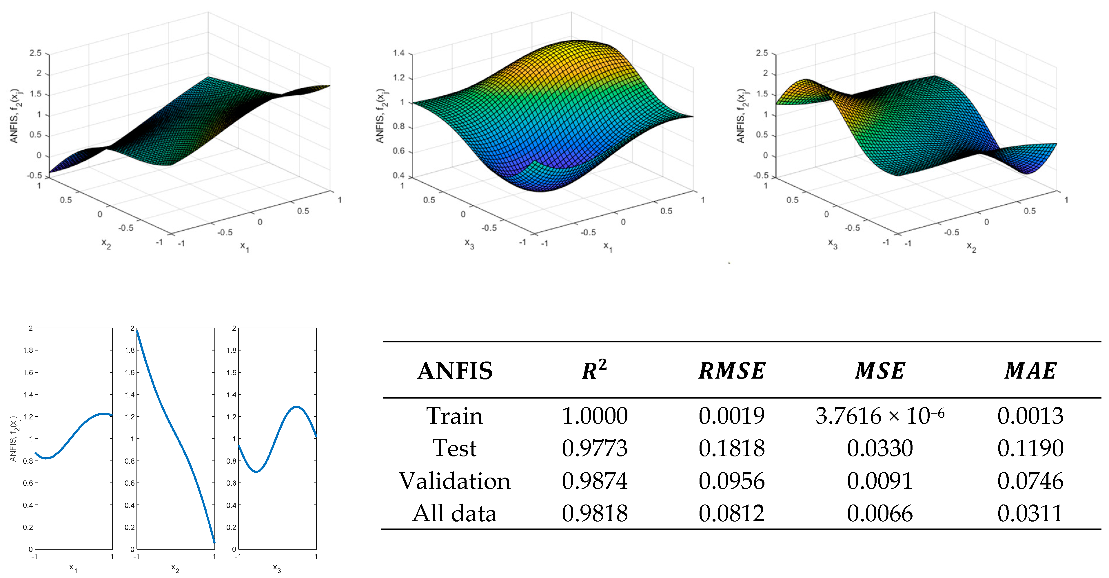
Figure 30 shows that it is possible to properly model the
function using the methodology proposed in this present study. Furthermore, as can be seen in
Figure 16 and
Figure 30, although the values provided by the validation metrics by using the ANN
3-4-2-1 are slightly better than those obtained by using the ANFIS, the ANFIS is able to approximate the actual shape of the function better than the neural network.
4.5. Analysis of an Actual Study Case
Once the previous
(type 1) and
(type 2) functions have been analyzed, a real case will be outlined, to assess whether the results obtained with the analytical function can be extrapolated to those obtained in a real case. To do this, the same methodology as previously shown will be used, i.e., the design will be divided into one part to train the models and into others for testing and validation. Subsequently, a modeling using RSM and soft computing techniques will be applied. These models will be fitted with the train data and will be validated and tested in the other data sets. The experiment number to select the data for train, test, and validation is the same as those previously used; however, they could be anyone. The actual data obtained in the die-sinking EDM of a Nickel and Chromium alloy using Cu-C electrodes and positive polarity have been taken from Ref. [
61]. Therefore, following the previously mentioned methodology, the experimental data are divided to 70%, 15%, and 15% for train, test, and validate, respectively. The train data will be used to obtain the models. A response surface model will be fitted first by using RSM and, secondly, soft computing tools (ANN and an ANFIS using the proposed method in
Section 4.4 of this present study) will be used.
The use of a methodology based on RSM allows modeling of the arithmetic average roughness of the roughness profile (Ra), but this is not the case of the EW, as shown in Ref. [
61]. From the determination coefficient of the regression shown in Ref. [
61], and from the classification that is followed in this present study, Ra (µm) could be classified as a type 1 function and EW (%) could be classified as a type 2 function, which can also be observed from
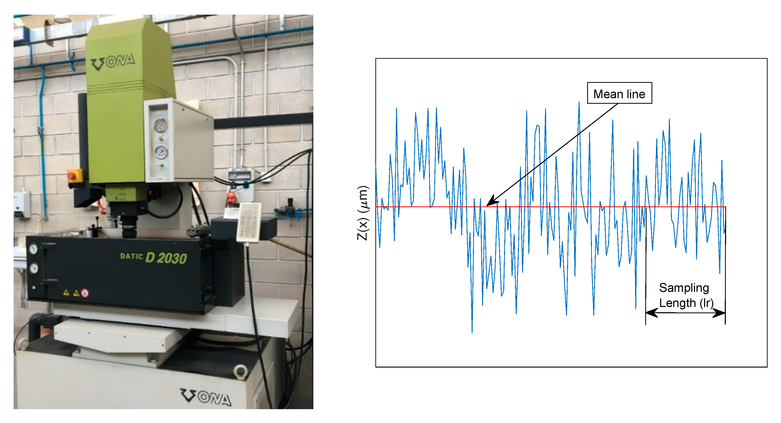
Figure 1. As is well-known
, is one of the most commonly employed parameters in industry and it is defined from the UNE-EN-ISO 4287:1999 norm [
69] as the arithmetic average roughness of the roughness profile, which is shown in
Figure 31, where the EDM equipment is also shown; and the EW is defined as the relation between the volume of material that is removed from the electrode and that removed from the part, which is usually expressed in %.
Figure 32 show a comparison between the results obtained, with the three methodologies analyzed in this present study (RSM, ANN, and ANFIS) and the actual results, for the case of Ra (µm), which as previously mentioned, could be considered to be a type 1 function, whose range of values is between [1.17 µm, 7.41 µm]. Likewise,
Figure 33 shows the validation metrics obtained with an ANFIS (
,
), ANN
3-8-1 and with the regression model for Ra values taken from Ref. [
61].
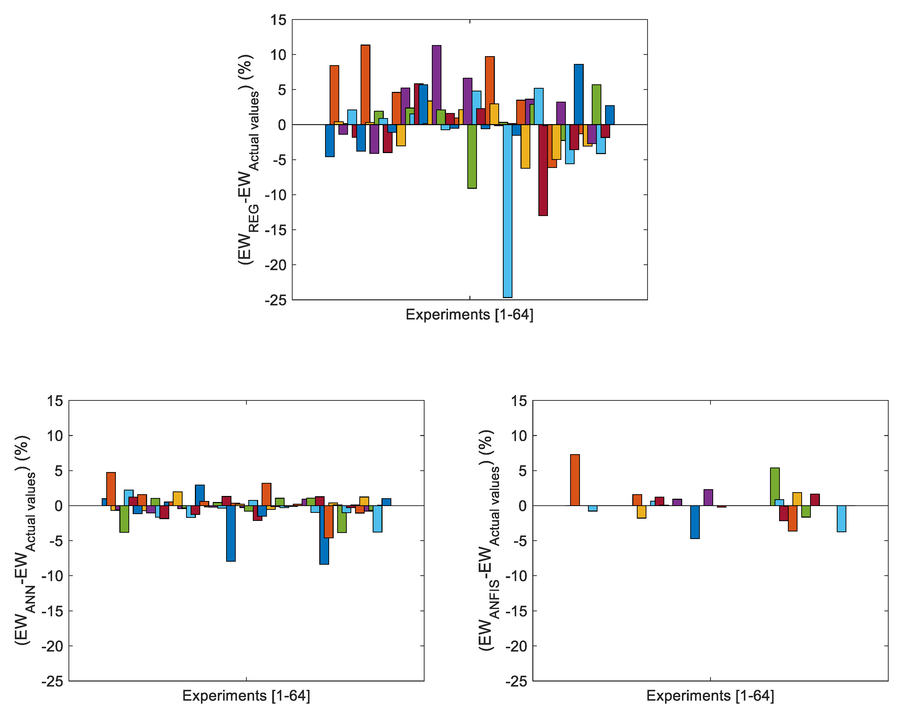
On the other hand,
Figure 34 show a comparison between the results obtained, with the three methodologies analyzed in this present study (RSM, ANN, and ANFIS) and the actual results, for the case of the EW (%), which could be considered to be a type 2 function, whose range of values is between [0.3%, 42.84%].
Figure 35 shows the validation metrics obtained with the ANFIS (
,
), ANN
3-5-2-1 and with the regression model for EW values taken from Ref [
61]. In the case of the EW, an ANN
3-5-2-1 was selected because the ANN
3-4-2-1 led to worse results.
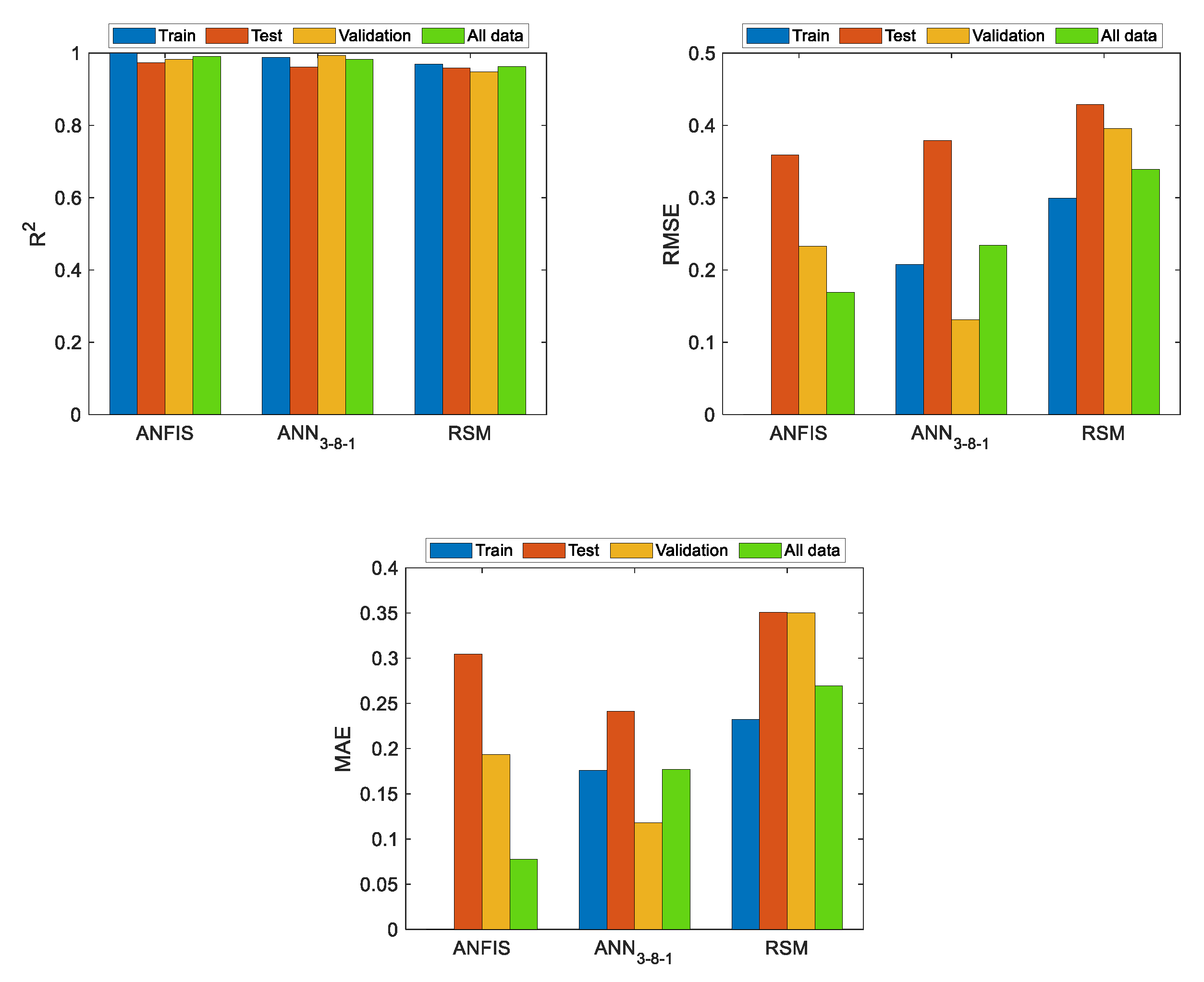
Figure 32,
Figure 33,
Figure 34 and
Figure 35 show the results obtained with the models fitted with the train data, but when these models are applied not only to the validation data but to all the experiments. As can be observed, both the ANFIS obtained with the proposed methodology and the ANNs present significant advantages over the regression models when there exists great variability in the data. Therefore, if there is a type 2 function, it is necessary to use models that allow greater precision to be obtained than that obtained with RSM. Furthermore, it can be observed that the ANFIS obtained from the proposed methodology have similar variability to the ANN and lower than the RSM when considering all experimental data.
5. Conclusions
In this present research study, two types of typologies that are usually found in the modeling of technological variables in manufacturing processes have been analyzed. These typologies have been denominated as type 1, with low variability in the response variable in relation to the independent variables, and type 2, with high variability in the response surface. A comparative study has been carried out between the precision of different models commonly used in Manufacturing Engineering, such as those based on RSM, ANN, and ANFIS, for modeling the behavior of technological variables.
It has been shown that response variables that correspond to typology 1 can be modeled by RSM. However, with modeling response variables that correspond to typology 2, it has been shown that the models obtained with conventional regression techniques based on RSM cannot adequately model the behavior of this kind of variables and therefore, in general, the results obtained are not accurate. Therefore, ANN or ANFIS-based techniques are highly effective in avoiding this problem. It has been shown that it is possible to use both neural networks and ANFIS to model the response variable with high accuracy. Both techniques allow the behavior of type 2 functions to be efficiently modeled.
In addition, in this present study a new methodology has been shown for obtaining a tuned FIS for modeling the behavior of both types of function topologies, which is based on the adjustment of the parameters of the membership functions that make up the FIS through an iterative process using an ANFIS for tuning the membership parameter of the thus generated FIS in order to minimize the MSE in the validation data. With this procedure, it has been shown that it is possible to obtain results with high precision for modeling both types 1 and 2 functions within the DOE range values.
The ANFIS obtained with the proposed methodology can provide better values of the validation metrics employed in this study in a better way than those obtained with both the RSM model and with the ANN that has 1 and 2 neurons in the hidden layer, and, the obtained results are similar to those obtained with the ANN that has 8 neurons in the hidden layer, when modeling the behavior of type 1 functions. Furthermore, when modeling type 2 functions, RSM was not able to accurately predict the behavior of the response variable. However, by using either an ANN or the methodology proposed in this present study, it was possible to accurately predict the behavior of this function.


