Abstract
In this paper, we integrate the autonomous search paradigm on a swarm intelligence algorithm in order to incorporate the auto-adjust capability on parameter values during the run. We propose an independent procedure that begins to work when it detects a stagnation in a local optimum, and it can be applied to any population-based algorithms. For that, we employ the autonomous search technique which allows solvers to automatically re-configure its solving parameters for enhancing the process when poor performances are detected. This feature is dramatically crucial when swarm intelligence methods are developed and tested. Finding the best parameter values that generate the best results is known as an optimization problem itself. For that, we evaluate the behavior of the population size to autonomously be adapted and controlled during the solving time according to the requirements of the problem. The proposal is testing on the dolphin echolocation algorithm which is a recent swarm intelligence algorithm based on the dolphin feature to navigate underwater and identify prey. As an optimization problem to solve, we test a machine-part cell formation problem which is a widely used technique for improving production flexibility, efficiency, and cost reduction in the manufacturing industry decomposing a manufacturing plant in a set of clusters called cells. The goal is to design a cell layout in such a way that the need for moving parts from one cell to another is minimized. Using statistical non-parametric tests, we demonstrate that the proposed approach efficiently solves 160 well-known cell manufacturing instances outperforming the classic optimization algorithm as well as other approaches reported in the literature, while keeping excellent robustness levels.
1. Introduction
Modern engineering tries to solve classical problems by combining new trends on technologies with traditional models. For example [1,2,3], mathematical models formulated by widely-known approaches are applied to improve industrial processes. In this context, the flexibility, efficiency, and productiveness appear as outstanding features in the current competitive manufacturing industries [4,5]. One of the most studied topics in this line of research is the manufacturing system. Developing cellular manufacturing systems is known to be an efficient way for handling those complex industry requirements. Competitive manufacturing industries have modeled their processes for managing the key resources in order to maximize their profits [6,7,8]. A crucial step for building these competitive systems is the machine-part cell formation (MPCF), which involves the decomposition of a manufacturing industry in completely independent clusters called cells. Those cells contain machines that process parts that share some features or belong to the same family. In an ideal decomposition, each cell is fully dedicated to a family of parts; however, often machines are required by two or more families. This leads to the generation of exceptional elements, that is, parts that need to visit different cells. Unfortunately, such a part flow among cells negatively impacts production times, inventory, and final costs among others [9]. As a consequence, the goal of the MPCF is to smartly design an industry decomposition into a set of cells in such a way the amount of exceptional elements is minimized.
Preliminary experiments were carried out by using classic exact methods such as linear programming [10,11]. Complete techniques are powerful techniques that employ an analysis of the entire search space to verify the global optimum value, and they often require a high amount of computational time and memory. For example, goal programming [12,13] is proposed as an exact method for solving this problem. In [14,15], the constraint programming paradigm is applied to the manufacturing cell design problem, and Ref. [16] includes the boolean satisfiability method for cell formation in group technology. As can be seen, these approaches are competitive when small and medium instances are solved. However, they take too long to solve the hardest instances [17]. For this reason, we believe that metaheuristics successfully work when a balance between the solving-time and good solutions is needed. In this context, metaheuristics as tabu search [18,19], simulated annealing [9], and particle swarm optimization [20] have become significant.
In this research, we solve the MPCF problem testing a swarm intelligence algorithm improved by a self-tuning component for improving the search process, increasing or decreasing the area of potential solutions. We propose a new procedure able to properly identify possible stagnation in a local optimal using information provided by the algorithm performance itself while it moves in the search space. This procedure is implemented by using modular architecture, and it is independent from the optimization algorithm. Therefore, it can be included in any population-based technique. To evaluate our procedure, we firstly employ the dolphin echolocation algorithm as a case study because parameter tuning has been not included in this algorithm yet. This algorithm is a method based on swarm intelligence that mimics the capabilities of dolphins, which employ their genetic sonar for direction-finding and hunting [21]. Such a sonar can emit high-frequency sounds called clicks to find prey. The algorithm represents the solutions as the dolphin positions, while the emission of clicks’ balances the exploration and exploitation capabilities of the metaheuristic. To reach the parameter setting paradigm on the dolphin echolocation algorithm, we use the promising capability belonging to Autonomous Search (AS) systems, which promotes the self-configuration of complex optimization solvers [22,23]. The main idea is to let the solver self-adjust some of its parameters in order to alleviate the parameter-setting work of programmers, which is known to be a tedious task, problem-dependent, and it is considered as an optimization problem itself. According to the No Free Lunch theorem [24], there is no general optimal metaheuristic parameter setting. It is not obvious to define a priori which parameter setting should be used. The optimal values for the parameters depend mainly on the problem and even the instance to deal with and on the search time that the user wants to spend on solving the problem. A universally optimal parameter value set for a given metaheuristic does not exist [25].
Based on this approach, the improved dolphin echolocation algorithm is able to autonomously adjust its population at runtime, according to its exhibited performance. We perform a set of experiments on 160 well-known MPCF instances where the proposed algorithm outperforms the classic algorithm as well as other metaheuristics reported in the literature while keeping excellent robustness levels.
The remainder of this paper is organized as follows: First, in Section 2, we present a literature review of the problem and several techniques to resolve it. Then, the machine-part cell formation with its mathematical model is explained in Section 3. Later, in Section 4, the dolphin echolocation algorithm is detailed. Next, our proposed variation is exposed in Section 5 explaining each one of its steps. Finally, the experimental results, statistical comparisons of results, and conclusions of this work are shown in Section 6 and Section 7, respectively.
2. Literature Review
The design of productive cells has had a large impact in the last two decades, due to the importance of establishing a strategy when organizing the location of each machine present in a manufactured industry. However, the interdependence of each productive cell makes it difficult for a product not to carry out transfers between cells. Therefore, the objective of the problem is to minimize the number of inter-cell movements to be able to finalize a product. In this context, several approaches have already been proposed, for instance, exact methods from the mathematical programming domain [10,11,12,13,26,27,28]. We may also find more modern exact methods such as constraint programming [15] and SAT [16]. In addition, exact methods combined with metaheuristics can also be found [29].
Now, considering metaheuristics for resolving the MPCF, we also find an extensive list of works devoted to manufacturing systems, principally using genetic algorithms. For instance, using a traditional approach [30], for the minimization of exceptional elements that conduces to a multi-objective optimization standpoint [31], mixed with discrete event simulation [32] to solve an MPCF mathematical model from the automobile industry, and combined with local search procedures [33].
Predator–prey as a variant of the classic genetic algorithm has also been reported [34], which proposes using as a fitness function a new grouping efficacy computation of cells. The scatter search method has been employed as well for solving manufacturing systems problems, but mostly oriented to multi-criteria group scheduling [35]. Classic simulated annealing [9], tabu search [18,19,36,37,38], and differential evolution [39] algorithms also present in the literature. These approaches are oriented to the grouping efficacy of cells in machine-part cell formation. A combination of particle swarm optimization and data mining techniques has also been used [20] to solve a well-known set of MPCF problems. More recent metaheuristics have also been employed to solve the this problem, for instance, a migrating birds algorithm is used to solve 90 classic MPCF problems efficiently [40]. An extended version of this work, where the several sorting processes of the metaheuristic are paralleled, has also been published [41]. Finally, another group of modern metaheuristics is proposed to solve this same set of problems efficiently, some examples are artificial fish swarm algorithms [42], shuffled frog leaping algorithms [43], bat algorithms [44], and flower and pollination algorithms [45].
Despite the long list of reported manuscripts being varied and extensive, currently few works are designed to solve this problem using a self-adjusting approach. This work is focused on improving the classic dolphin echolocation algorithm [46] by introducing autonomous search capabilities to the core algorithm, which is able to balance the amount of population required to different parts of the search space. We select this swarm intelligence method because a self-adaptive approach has not been proposed for this algorithm yet. In this context, we investigate a recent proposal about a simplification of the dolphin echolocation algorithm that it needs no empirical parameter to work [47]. In [48], a modified dolphin echolocation algorithm based on the creation of the basic collapse mechanisms, and it is proposed to optimize analysis of plastic structures. This work verifies the efficiency of the algorithm by comparing results with exact solutions. Similar work can be seen in [49] where again an improved dolphin echolocation algorithm is developed to solve a complex optimization problem.
Using statistical non-parametric tests, we compare the results with the classic algorithm and several other metaheuristics, illustrating the efficiency of our AS algorithm. We additionally analyze a larger and more complex set of instances composed of 160 benchmarks, providing new bounds for a subset of instances whose global optimum is currently unknown.
3. Problem Statement
As previously explained, the MPCF consists of organizing a factory plant in productive cells, where each cell contains machines that process product parts. The idea is to minimize the so-called exceptional elements, which are indeed parts that move from one cell to another to satisfy the production workflow [27]. The mathematical model representing this problem is described as follows:
- Indices.
- -
- i: machine type, }.
- -
- j: part type, .
- -
- k: cell type, }.
- Parameters.
- -
- M: the number of machines.
- -
- P: the number of parts.
- -
- C: the number of cells.
- -
- : the maximum number of machines per cell.
- Variables.
- -
- : the binary machine-part incidence matrix, where:
- -
- : the binary machine-cell incidence matrix, where:
- -
- : the binary part-cell incidence matrix, where:
The objective function is given by:
subject to:
An example of binary machine-part incidence matrix is depicted in Figure 1 together with its corresponding ideal configuration, where no exceptional elements are present.
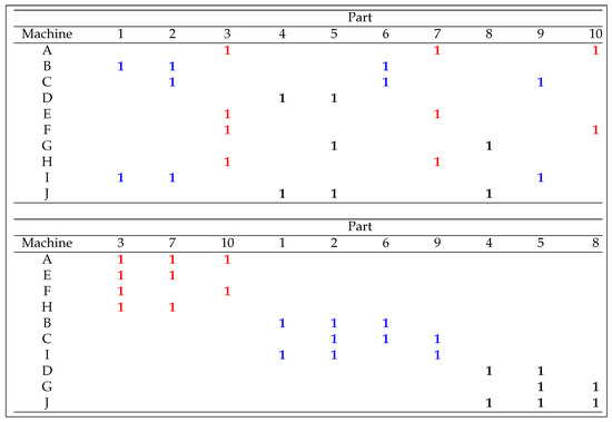
Figure 1.
Initial and ideal incidence machine-part matrices.
This organization is built using the solution of the problem, which is given by the binary machine-cell incidence matrix depicted on the left side of Figure 2. Machines B, C, and I are stated in cell 1; the machines D, G, and J in cell 2; the machines A, E, F, and H in cell 3. An analogous representation of this matrix is depicted in Figure 2, which is employed in this paper as it allows for avoiding the generation of unfeasible solutions when the same machine is assigned to more than one cell by the metaheuristic.
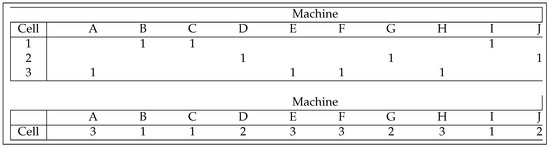
Figure 2.
Two solution representations for the machine-cell matrix.
4. Dolphin Echolocalization Algorithm
Echolocation is an interesting exploration system present in some species of the animal kingdom. One of them is the dolphin, which smartly uses this feature for locating objects over the sea, particularly its prey. The dolphin echolocation operates by the emission of sounds, called clicks, and echoes. Once the dolphin emits a click, an echo is returned when an object is hit by the sound. The time interval between the click emission and echo reception is used by the dolphin to evaluate the distance from the prey. Using this capability, the dolphin is able to track an object by continuously emitting clicks and receiving its corresponding echo. The dolphin echolocation metaheuristic mimics those behaviors and a general procedure of the algorithm is depicted in Algorithm 1.
- Parameters of the algorithm.
- -
- : Maximum number of iterations (stop criteria).
- -
- : The number of locations. Each location will correspond to a potential solution of the problem.
- -
- : The effective radius of search. This parameter is used to calculate the accumulated fitness of the problem.
- -
- : The degree of the convergence curve.
| Algorithm 1: Dolphin echolocation algorithm. |
 |
The first phase of the algorithm is to sort in ascending or descending order the search space of the problem. To this end, a matrix of alternatives is created. Then, for each decision variable j, an associated vector is created that holds the possible alternatives for j. Vectors for each decision variable are grouped forming the matrix, where is , and is the number of variables of the problem. Then, random dolphin locations (solutions) are produced and then stored in a matrix. For the present problem, each solution is composed of a set of machines assigned to cells as depicted in Figure 2.
On line 3, a while loop encloses a set of actions to be performed until the stop criterion is met. An interesting feature of the dolphin echolocation algorithm is the capability of balancing exploration and exploitation capabilities by a user-defined convergence factor. Indeed, the convergence curve on which the process should operate is defined by Equation (5):
where is the predefined probability, is the convergence factor of the first iteration, is the iteration i, and is the number of iterations. Once is computed, the fitness for each location must be calculated. On line 6, the accumulative fitness is computed according to Algorithm 2.
where defines the accumulative fitness of the th alternative for variable j. The autonomous search method will be detailed in the next section.
| Algorithm 2: Calculate accumulative fitness. |
 |
Once the accumulative fitness is computed, the best location must be encountered, and the alternatives allocated to the variables of the best location in the matrix are set to zero, as shown in Algorithm 3.
| Algorithm 3: Restart AF values. |
 |
5. Autonomous Search
The basic version of the dolphin echolocation algorithm does not have capability for controlling its parameters. If the behavior of (numbers of location) is studied, we can see that it is valuated before the run of the metaheuristic. When the loop statement of the algorithm is running, the potential solutions are modified updating their location. However, the total number of solutions remains unchanged.
On the one hand, we can observe that the second part of the metaheuristic uses a reset process for the accumulate function. It is a static procedure and it is influenced by the best solution, resting always according to the best location (solution). On the other hand, in the third part of the algorithm, the assignment of probabilities is controlled by condition if the alternative is equal to the best location. Again, the best solution dramatically impacts the performance of the procedure. For both cases, that thought is not necessarily successful, since often a bad solution, sometimes, can lead the search to the global best solution.
These concerns are very important for the efficiently of the algorithm, the reason why we have decided to create an autonomous system approach for evaluating and calculating the value of the in an autonomous way. For that, we use autonomous search, which is a particular case of adaptive systems that improve their solving performance by modifying and adjusting themselves to the problem at hand, either by adaptation or supervised adaptation [22,50]. This approach has successfully been applied in constraint programming using bio-inspired algorithms [51] for controlling the process resolution of solver tools [52]. The objective of autonomous search is to allow the metaheuristic to self-adapt the value of the parameter during the run, according to the algorithm convergence.
Recent works illustrating how to improve evolutionary algorithms by dynamically controlling parameters during solving time can be seen in [53,54,55,56,57,58]. Analyzing these works, we have considered to modify the original dolphin echolocation algorithm taking the autonomous search principles for creating a procedure that adaptively vary the number of potential solutions ( parameter), according to the exhibited efficiency during the search process. The dolphin echolocation algorithm involves at least four parameters, but we vary only the parameter because, in a previous sample phase, we observe that this component dramatically impacts the performance of the algorithm. On the other hand, we are convinced that measuring the quality of an autonomous multi-proposal is complicated, due to the fact that there would be no clarity on which parameter gives the best result. As a consequence, we will have a much more straightforward implementation.
We believe this approach also provides know-how for future experiments involving adaptive population for population-based algorithms. The procedure is described in Algorithm 4. Inputs of the procedure are: the number of location , the number of variables , current iteration t, and number of stagnation that represents the number of iterations where the best solution does not improve, commonly called “local search”.
| Algorithm 4: Adaptive approach for the NL parameter. |
 |
Now, we calculate the difference between best and worst solutions, according to the cost of each one and then it is divided by the sum of all costs (Line 2). This value describes the percentage () of maximum separation between solutions. A low percentage value indicates that solutions are homogeneous skewed to the best solution, in which case the procedure creates new solutions (Lines 4–18). To create these solutions, we reuse the percentage to determinate if they are cloned from best solution (Lines 8–10) or they are randomly generated (Lines 13–17). On the other hand, if means that solutions are heterogeneous, thus the procedure removes the worst solutions (Lines 21–24). In both cases, the percentages calculated can also be seen as a mechanism to support the exploration and exploitation phases. If solutions are homogeneous, this procedure allows for exploring towards new solutions, while, if solutions are heterogeneous, the procedure converges towards a set of similar solutions itself.
Finally, we implement Algorithm 4 for parameter tuning in a modular manner. If we closely analyze this procedure, we can note that it operates independently of the main process of the metaheuristic. When the dolphin echolocation algorithm is caught in a local optimal, the adaptive approach is invoked to modify the population. In this context, we guarantee that this module can be included as a plug and play plugin in more than 80 population-based metaheuristics [59] without an over-effort. In this sense, the proposed contribution is framed to a more broad approach.
6. Experimental Results
In order to evaluate the performance of the autonomous algorithm, we have used two sets of the machine-part cell formation, the first consisting of 90 instances proposed by Boctor [27], while the second consists of 70 new instances which have a higher level of complexity. Parameter setting is known to be a complex task, itself being recognized as an optimization problem. To select the parameters of the algorithm, we performed a sampling test. Best results were obtained using the following configuration taken from [60]:
- Number locations (): 10.
- Number loops (): 2000.
- Effective radius (): 1.
- Convergence factor (): .
- Degree of the curve (): 1.
- Local search (): 20.
We performed variations only on the number of locations, due to its high level of impact on the efficiency of the algorithm. Autonomous search indicates the changes that must be made will depend on the performance of the algorithm in measurable periods. Thus, we can establish as a premise: “a better quality of solutions leads to an increase in the number of solutions, while a lower quality of solutions means a decrease in the number of solutions”.
Our approach has been implemented in Java 1.8 and run in a computer with an Intel Core i5 6600 k 3500 MHz processor, 8 GB RAM DDR4 2133 MHz with Windows 10 64 bits as an operating system.
6.1. Boctor Problems
For testing, Boctor refers to 10 basic problems which come out in 90 different instances, where there are instances with two and three numbers of cells. In the first one, the maximum number of machines per cell () varies between 8 and 12. The second one presents variations between 6 and 9. Each of these instances will be described in Table 1 where it is assigned an identifier number for each of them.

Table 1.
Boctor instances.
In this experiment, population variations were performed every 31 iterations, making increases and decreases randomly. In order to measure the performance of the modified algorithm, comparisons were made with the original algorithm, establishing fixed populations of , which seeks to establish similar conditions to those presented by the modified Dolphin Echolocation Algorithm. The obtained results can be seen in Table 2.
Table 2.
Boctor and AS results. For space reasons, we renamed I instead of .
We already have used metrics to successfully evidence the performance of algorithms [52,61,62,63,64]. In this case study, we employ a similar formulation to measure the potential of the adaptive approach:
- The time was established in milliseconds (t) to reach the global optimum.
- We used the number of iterations () necessary to obtain the global optimum.
- We will use the robustness of the algorithm which is represented by the following formula:
Within the obtained results, it can be seen that the conjunction of autonomous search with dolphin echolocation algorithm has achieved in of the cases to reach a robustness. The experiments that were executed by the original algorithm obtained the following results, , only 10 instances managed to obtain a robustness greater than ; , 32 instances reached a percentage equal to the previous one; , 50 instances obtained a robustness greater than ; , 52 instances reached a percentage higher than ; , 48 instances managed to overcome a robustness of ; , 8 instances achieved robustness, which means of the experiments performed. However, this is achieved with a significant amount of time and needed to reach the global optimum. On the other hand, in of the cases, the autonomous approach managed to obtain smaller execution times and quantity than the original algorithm. However, with , similar times and were obtained due to the small amount of population. However, its robustness is largely affected.
With the obtained results, it can be established that, when using the technique of autonomous search, the optimal solution is reached in a smaller amount of time and , which can be observed in Figure 3 and Figure 4. On the other hand, Figure 5 shows the robustness of the algorithm, which is increased when using autonomous search. However, after updating the population with the same robustness increments, but with a higher number of and execution time.
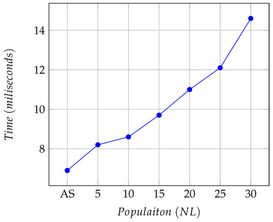
Figure 3.
Average of Runtime.
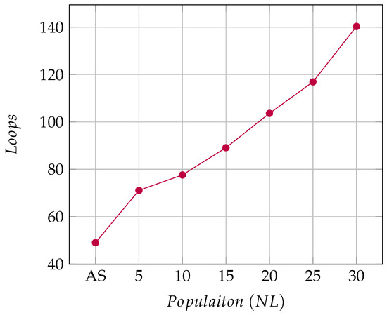
Figure 4.
Average of .
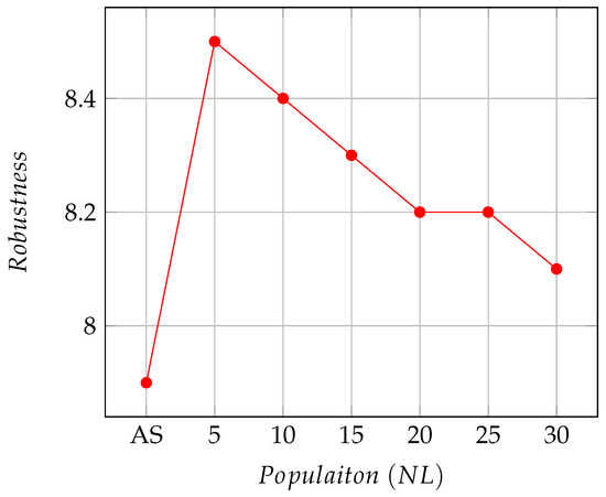
Figure 5.
Average of Robustness.
6.2. Other Instances
To reaffirm the performance of the autonomous dolphin echolocation algorithm, proceed to a new phase of experimentation with problems of a greater degree of difficulty, which consists of 70 new instances depicted in Table 3.
Table 3.
Hardest instances.
As in previous experiments, population changes are performed every 20 iterations (local search number , defined at the beginning of this section), which consist of increases or decreases in the number of locations, according to Algorithm 4. To validate the performance of the technique used, it will be compared with the original algorithm, with fixed populations of and , in order to establish similar conditions. The obtained results are presented in Table 4.
Table 4.
Hardest instances and AS results. For space reasons, we renamed I instead of .
To measure the performance of the solution, we use the following metrics:
- Determining the execution time necessary to reach the global optimum, which is expressed in milliseconds.
- The best optimal found (x).
- Using Equation (6) to show the robustness () of the obtained results.
Through the obtained results, it is possible to affirm that an autonomous approach obtained in 90% of the cases proposed 100% of the robustness. On the other hand, the experiments that were executed by the original algorithm obtained the following results: when , only 32% achieved 100%; if , then 37%; for , 40% cases are successful; in the case of , the percentage with good results achieves a maximum of 46% while outperforms 58%. Finally, the best results are given by , where it is able to resolve 140 instances, equivalent to 87% of total. However, these results need a longer execution time compared to the modified algorithm. Although our proposal is better than all configurations of the original version, due to it finding almost 90% of the known optimal, its solving time is overcome by the original version because of the fact that it includes an extra computational-time to the self-adjustment of the .
Results allow asserting that using the proposed autonomous approach for the dolphin echolocation algorithm to solve the machine-part cell formation problem is an efficient alternative. We can see that this improvement reaches global optima in a shorter amount of time (see Figure 6). More evidence of the performance of the algorithm is illustrated in Figure 7.
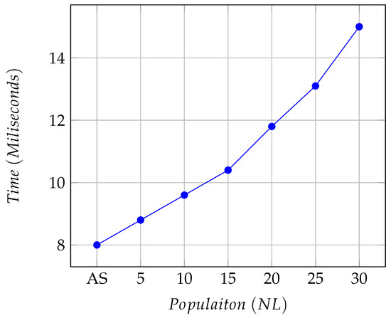
Figure 6.
Average of Runtime.
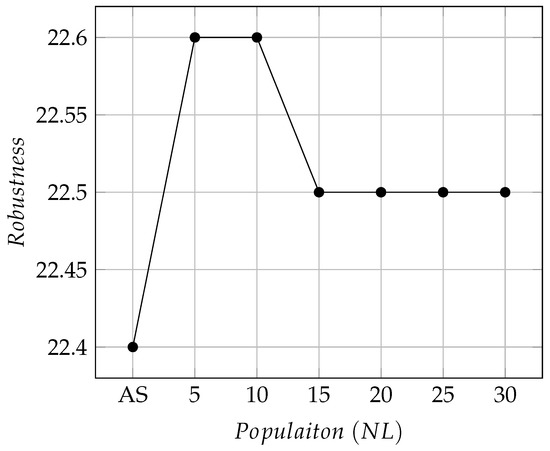
Figure 7.
Average of Robustness.
6.3. Statistical Analysis
To test a significant difference between the original version of the Dolphin Echolocation Algorithm and our autonomous proposal, we tested with a statistical test for each instance through the Kolmogorov–Smirnov–Lilliefors. This test allows us to determine if samples are independent [78], and then we use Wilcoxon’s signed rank [79] for statistically comparing the results. For this evaluation, the basic dolphin echolocation algorithm with was used, due to it reporting better results.
For the Kolmogorov–Smirnov–Lilliefors test, we consider a hypothesis evaluation (p-value ≤ 0.05), smaller values that determine that the null hypothesis will be reject. For the Wilcoxon’s signed rank, we observe the averages of each instance and discover that there is not a significant difference between the results of both approaches. This leads us to decrease the levels of significance (p-value ≤ 0.01), and thus it has a higher precision. Both tests were conducted using GNU Octave [80].
The Kolmogorov–Smirnov–Lilliefors test is necessary to study the independence of samples by determining if the reaches from the 31 executions of each instance describe a Gaussian distribution. For that, we use as null hypotheses which states that follows a normal distribution. The alternative hypotheses state the opposite. We perform the test to demonstrate the alternative hypothesis. The obtained result for the p-value was ; then, must be rejected. This evidence implies that applying the central limit theorem is not viable. Then, as the samples are not distributed normally, we have chosen a non-parametric statistical hypothesis test, Wilcoxon’s signed rank to compare these results. For the Wilcoxon’s signed rank test, describes the null hypotheses and it states that achieved by our autonomous approach is better than achieved by the dolphin echolocation algorithm.
Table 5 and Table 6 compare the original algorithm versus the autonomous approach, for all tested instances via the Wilcoxon’s signed rank test. As the significance level is also established to , smaller values that defines that cannot be assumed. To know the winner, it is enough to observe the row of the instance and identify the column where the p-value exists, for example in the problem 4 (Boctor 01), the autonomous approach is better than the basic DEA because its value is lower than , then cannot be assumed. In the other cases, there is no information.
Table 5.
Statistical test. DEA vs. Autonomous approach solving the Boctor instance.
Table 6.
Statistical test. DEA vs. Autonomous approach solving the hardest instance.
According to results in the 90 first instances, for p-value lower than (p-value ≤ 0.01) for the original dolphin echolocation algorithm are 0, for the autonomous approach are 78. The rest of tests do not provide significant information, due to p-values being greater than , but less than , or samples are equal. Now, considering the 70 hard instances, the original dolphin echolocation algorithm achieves 1 p-value lower than , while our autonomous approach reaches 1 p-value below . For the rest of the tests, p-values are not significant or, again, samples are equal.
Summarizing, we can note that the improved algorithm exhibits a better performance concerning its basic version only in the smaller Doctor’s instances and a few of the hardest instances. We believe this behavior is due to the native algorithm operating appropriately when it faces complex optimization problems. However, as previously mentioned, our proposed self-adaptive algorithm can be considered a contribution itself and it can be applied to a wide set of population-based methods.
7. Conclusions
In this research, we have presented an adaptive procedure that allows for identifying a stagnation in a local optimal. This feature appears when the variability of solutions is required to explore different feasible regions of an optimization problem. The technique is implemented via modular architecture and it is independent of the optimization algorithm, and therefore it can be included in any population-based method. To test this approach, we employ the dolphin echolocation algorithm to solve different instances of the machine-part cell formation. This approach is inspired by the online control for number location parameter which is valuated before the run of the metaheuristic. To this end, we use an autonomous search that is a particular case of adaptive systems that improve their solving performance by modifying and adjusting themselves to the problem at hand, either by adaptation or supervised adaptation. We have tested two sets of the machine-part cell formation, the first one consisted of 90 instances proposed by Boctor, while the second one included 70 new hard instances, where several global optimum values that were not reached using the basic dolphin echolocation algorithm were achieved via the auto-adaptive approach. We have also compared the proposed adaptive approach by using a nonparametric statistical tests and the results are conclusive. As a conclusion, and as a way to compare the methods, the use of the autonomous search technique on the dolphin echolocation algorithm causes positive impacts on it, decreasing time and loops, with a considerable increase in robustness.
As future work, we plan to experiment auto-adaptive approaches in recent bio-inspired algorithms and to provide a larger comparison of techniques for solving the machine-part cell formation. The integration of autonomous search can lead the research toward new study lines, such as dynamically selecting the best binarization strategy during solving according to performance indicators as analogously studied in [81].
Author Contributions
Formal analysis, R.O. and C.C. (Cécar Carrasco); investigation, R.S., B.C., R.O., H.d.l.F.-M., and E.R.-T.; methodology, R.S. and B.C.; resources, R.S. and B.C.; software, R.O. and C.C. (Cécar Carrasco); validation, H.d.l.F.-M. and E.R.-T., F.P., C.C. (Carlos Castro), and R.O.; writing—original draft, C.C. (Cécar Carrasco); writing—review and editing, R.S., B.C., E.R.-T., and H.d.l.F.-M. All the authors of this paper hold responsibility for every part of this manuscript. All authors have read and agreed to the published version of the manuscript.
Funding
Ricardo Soto is supported by Grant CONICYT/FONDECYT/REGULAR/1190129. Broderick Crawford is supported by Grant CONICYT/FONDECYT/REGULAR/1171243. Hanns de la Fuente-Mella, Ricardo Soto, and Broderick Crawford are supported by Grant Nucleo de Investigacion en Data Analytics/VRIEA/PUCV/039.432/2020.
Conflicts of Interest
The authors declare no conflict of interest. The founding sponsors had no role in the design of the study; in the collection, analyses, or interpretation of data; in the writing of the manuscript, and in the decision to publish the results.
References
- Božek, P.; Ivandić, Ž.; Lozhkin, A.; Lyalin, V.; Tarasov, V. Solutions to the characteristic equation for industrial robot’s elliptic trajectories. Teh. Vjesn. Tech. Gaz. 2016, 23. [Google Scholar] [CrossRef]
- Božek, P.; Al Akkad, M.A.; Blištan, P.; Ibrahim, N.I. Navigation control and stability investigation of a mobile robot based on a hexacopter equipped with an integrated manipulator. Int. J. Adv. Robot. Syst. 2017, 14. [Google Scholar] [CrossRef]
- Kilin, A.; Božek, P.; Karavaev, Y.; Klekovkin, A.; Shestakov, V. Experimental investigations of a highly maneuverable mobile omniwheel robot. Int. J. Adv. Robot. Syst. 2017, 14. [Google Scholar] [CrossRef]
- Zhang, Z. Modeling complexity of cellular manufacturing systems. Appl. Math. Model. 2011, 35, 4189–4195. [Google Scholar] [CrossRef]
- Gu, P.; Monid, A. Design of cellular manufacturing systems. An industrial case study. Robot. Comput. Integr. Manuf. 1993, 10, 147–151. [Google Scholar] [CrossRef]
- Ah kioon, S.; Bulgak, A.A.; Bektas, T. Integrated cellular manufacturing systems design with production planning and dynamic system reconfiguration. Eur. J. Oper. Res. 2009, 192, 414–428. [Google Scholar] [CrossRef]
- Saxena, L.K.; Jain, P.K. Dynamic cellular manufacturing systems design—A comprehensive model. Int. J. Adv. Manuf. Technol. 2011, 53, 11–34. [Google Scholar] [CrossRef]
- De la Fuente-Mella, H.; Rojas Fuentes, J.L.; Leiva, V. Econometric modeling of productivity and technical efficiency in the Chilean manufacturing industry. Comput. Ind. Eng. 2020, 139, 105793. [Google Scholar] [CrossRef]
- Wu, T.H.; Chang, C.C.; Chung, S.H. A simulated annealing algorithm for manufacturing cell formation problems. Expert Syst. Appl. 2008, 34, 1609–1617. [Google Scholar] [CrossRef]
- Purcheck, G.F.K. A Linear–programming method for the combinatorial grouping of an incomplete power set. J. Cybern. 1975, 5, 51–76. [Google Scholar] [CrossRef]
- Oliva-Lopez, E.; Purcheck, G. Load balancing for group technology planning and control. Int. J. Mach. Tool Des. Res. 1979, 19, 259–274. [Google Scholar] [CrossRef]
- Sankaran, S.; Rodin, E.Y. Multiple objective decision-making approach to cell formation: A goal programming model. Math. Comput. Model. 1990, 13, 71–81. [Google Scholar] [CrossRef]
- Shafer, S.M.; Rogers, D.F. A goal programming approach to the cell formation problem. J. Oper. Manag. 1991, 10, 28–43. [Google Scholar] [CrossRef]
- Soto, R.; Kjellerstrand, H.; Gutiérrez, J.; López, A.; Crawford, B.; Monfroy, E. Solving manufacturing cell design problems using constraint programming. In Advanced Research in Applied Artificial Intelligence; Springer: Berlin/Heidelberg, Germany, 2012; pp. 400–406. [Google Scholar] [CrossRef]
- Soto, R.; Crawford, B.; Almonacid, B.; Paredes, F.; Loyola, E. Machine-part cell formation problems with constraint programming. In Proceedings of the 2015 34th International Conference of the Chilean Computer Science Society (SCCC), Santiago, Chile, 9–13 November 2015. [Google Scholar] [CrossRef]
- Soto, R.; Kjellerstrand, H.; Durán, O.; Crawford, B.; Monfroy, E.; Paredes, F. Cell formation in group technology using constraint programming and Boolean satisfiability. Expert Syst. Appl. 2012, 39, 11423–11427. [Google Scholar] [CrossRef]
- Almonacid, B.; Aspée, F.; Soto, R.; Crawford, B.; Lama, J. Solving the manufacturing cell design problem using the modified binary firefly algorithm and the egyptian vulture optimisation algorithm. IET Softw. 2017, 11, 105–115. [Google Scholar] [CrossRef]
- Aljaber, N.; Baek, W.; Chen, C.L. A tabu search approach to the cell formation problem. Comput. Ind. Eng. 1997, 32, 169–185. [Google Scholar] [CrossRef]
- Lozano, S.; Adenso-Diaz, B.; Eguia, I.; Onieva, L. A one-step tabu search algorithm for manufacturing cell design. J. Oper. Res. Soc. 1999, 50, 509. [Google Scholar] [CrossRef]
- Durán, O.; Rodriguez, N.; Consalter, L.A. Collaborative particle swarm optimization with a data mining technique for manufacturing cell design. Expert Syst. Appl. 2010, 37, 1563–1567. [Google Scholar] [CrossRef]
- Wu, T.Q.; Yao, M.; Hua Yang, J. Dolphin swarm algorithm. Front. Inf. Technol. Electron. Eng. 2016, 17, 717–729. [Google Scholar] [CrossRef]
- Hamadi, Y.; Monfroy, E.; Saubion, F. What is autonomous search? In Hybrid Optimization; Springer: New York, NY, USA, 2010; pp. 357–391. [Google Scholar] [CrossRef]
- Huang, C.; Li, Y.; Yao, X. A survey of automatic parameter tuning methods for metaheuristics. IEEE Trans. Evol. Comput. 2020, 24, 201–216. [Google Scholar] [CrossRef]
- Wolpert, D.; Macready, W. No free lunch theorems for optimization. IEEE Trans. Evol. Comput. 1997, 1, 67–82. [Google Scholar] [CrossRef]
- Talbi, E.G. Metaheuristics: From Design to Implementation; John Wiley & Sons: Hoboken, NJ, USA, 2009. [Google Scholar]
- Kusiak, A.; Chow, W.S. Efficient solving of the group technology problem. J. Manuf. Syst. 1987, 6, 117–124. [Google Scholar] [CrossRef]
- Boctor, F.F. A jinear formulation of the machine-part cell formation problem. Int. J. Prod. Res. 1991, 29, 343–356. [Google Scholar] [CrossRef]
- Albadawi, Z.; Bashir, H.A.; Chen, M. A mathematical approach for the formation of manufacturing cells. Comput. Ind. Eng. 2005, 48, 3–21. [Google Scholar] [CrossRef]
- Boulif, M.; Atif, K. A new branch-&-bound-enhanced genetic algorithm for the manufacturing cell formation problem. Comput. Oper. Res. 2006, 33, 2219–2245. [Google Scholar] [CrossRef]
- Venugopal, V.; Narendran, T. A genetic algorithm approach to the machine-component grouping problem with multiple objectives. Comput. Ind. Eng. 1992, 22, 469–480. [Google Scholar] [CrossRef]
- Gupta, Y.; Gupta, M.; Kumar, A.; Sundaram, C. A genetic algorithm-based approach to cell composition and layout design problems. Int. J. Prod. Res. 1996, 34, 447–482. [Google Scholar] [CrossRef]
- Imran, M.; Kang, C.; Lee, Y.H.; Jahanzaib, M.; Aziz, H. Cell formation in a cellular manufacturing system using simulation integrated hybrid genetic algorithm. Comput. Ind. Eng. 2017, 105, 123–135. [Google Scholar] [CrossRef]
- Nsakanda, A.L.; Diaby, M.; Price, W.L. Hybrid genetic approach for solving large-scale capacitated cell formation problems with multiple routings. Eur. J. Oper. Res. 2006, 171, 1051–1070. [Google Scholar] [CrossRef]
- Banerjee, I.; Das, P. Group technology based adaptive cell formation using predator–prey genetic algorithm. Appl. Soft Comput. 2012, 12, 559–572. [Google Scholar] [CrossRef]
- Tavakkoli-Moghaddam, R.; Javadian, N.; Khorrami, A.; Gholipour-Kanani, Y. Design of a scatter search method for a novel multi-criteria group scheduling problem in a cellular manufacturing system. Expert Syst. Appl. 2010, 37, 2661–2669. [Google Scholar] [CrossRef]
- Chang, C.C.; Wu, T.H.; Wu, C.W. An efficient approach to determine cell formation, cell layout and intracellular machine sequence in cellular manufacturing systems. Comput. Ind. Eng. 2013, 66, 438–450. [Google Scholar] [CrossRef]
- Lei, D.; Wu, Z. Tabu search-based approach to multi-objective machine-part cell formation. Int. J. Prod. Res. 2005, 43, 5241–5252. [Google Scholar] [CrossRef]
- Chung, S.H.; Wu, T.H.; Chang, C.C. An efficient tabu search algorithm to the cell formation problem with alternative routings and machine reliability considerations. Comput. Ind. Eng. 2011, 60, 7–15. [Google Scholar] [CrossRef]
- Noktehdan, A.; Karimi, B.; Kashan, A.H. A differential evolution algorithm for the manufacturing cell formation problem using group based operators. Expert Syst. Appl. 2010, 37, 4822–4829. [Google Scholar] [CrossRef]
- Soto, R.; Crawford, B.; Almonacid, B.; Paredes, F. A migrating birds optimization algorithm for machine-part cell formation problems. In Advances in Artificial Intelligence and Soft Computing: 14th Mexican International Conference on Artificial Intelligence, MICAI 2015, Cuernavaca, Morelos, Mexico, 25–31 October 2015, Proceedings, Part I; Springer: Cham, Switzerland, 2015; pp. 270–281. [Google Scholar] [CrossRef]
- Soto, R.; Crawford, B.; Almonacid, B.; Paredes, F. Efficient parallel sorting for migrating birds optimization when solving machine-part cell formation problems. Sci. Program. 2016, 2016, 9402503. [Google Scholar] [CrossRef]
- Soto, R.; Crawford, B.; Vega, E.; Paredes, F. Solving manufacturing cell design problems using an artificial fish swarm algorithm. In Advances in Artificial Intelligence and Soft Computing: 14th Mexican International Conference on Artificial Intelligence, MICAI 2015, Cuernavaca, Morelos, Mexico, 25–31 October 2015, Proceedings, Part I; Springer: Cham, Switzerland, 2015; pp. 282–290. [Google Scholar] [CrossRef]
- Soto, R.; Crawford, B.; Vega, E.; Johnson, F.; Paredes, F. Solving manufacturing cell design problems using a shuffled frog leaping algorithm. In The 1st International Conference on Advanced Intelligent System and Informatics (AISI2015), 28–30 November 2015, Beni Suef, Egypt; Springer: Cham, Switzerland, 2016; pp. 253–261. [Google Scholar] [CrossRef]
- Soto, R.; Crawford, B.; Alarcón, A.; Zec, C.; Vega, E.; Reyes, V.; Araya, I.; Olguín, E. Solving manufacturing cell design problems by using a bat algorithm approach. In Advances in Swarm Intelligence: 7th International Conference, ICSI 2016, Bali, Indonesia, 25–30 June 2016, Proceedings, Part I; Springer: Cham, Switzerland, 2016; pp. 184–191. [Google Scholar] [CrossRef]
- Soto, R.; Crawford, B.; Olivares, R.; De Conti, M.; Rubio, R.; Almonacid, B.; Niklander, S. Resolving the manufacturing cell design problem using the flower pollination algorithm. In Multi-Disciplinary Trends in Artificial Intelligence: 10th International Workshop, MIWAI 2016, Chiang Mai, Thailand, 7–9 December 2016, Proceedings; Springer: Cham, Switzerland, 2016; pp. 184–195. [Google Scholar] [CrossRef]
- Soto, R.; Crawford, B.; Carrasco, C.; Almonacid, B.; Reyes, V.; Araya, I.; Misra, S.; Olguín, E. Solving manufacturing cell design problems by using a dolphin echolocation algorithm. In Computational Science and Its Applications—ICCSA 2016; Springer: Cham, Switzerland, 2016; pp. 77–86. [Google Scholar] [CrossRef]
- Kaveh, A.; Vaez, S.R.H.; Hosseini, P. Simplified dolphin echolocation algorithm for optimum design of frame. Smart Struct. Syst. 2018, 21, 321–333. [Google Scholar] [CrossRef]
- Daryan, A.S.; Palizi, S.; Farhoudi, N. Optimization of plastic analysis of moment frames using modified dolphin echolocation algorithm. Adv. Struct. Eng. 2019, 22, 2504–2516. [Google Scholar] [CrossRef]
- Gholizadeh, S.; Poorhoseini, H. Seismic layout optimization of steel braced frames by an improved dolphin echolocation algorithm. Struct. Multidiscip. Optim. 2016, 54, 1011–1029. [Google Scholar] [CrossRef]
- Hamadi, Y.; Monfroy, E.; Saubion, F. An introduction to autonomous search. In Autonomous Search; Springer: Berlin/Heidelberg, Germany, 2011; pp. 1–11. [Google Scholar] [CrossRef]
- Soto, R.; Crawford, B.; Olivares, R.; Niklander, S.; Johnson, F.; Paredes, F.; Olguín, E. Online control of enumeration strategies via bat algorithm and black hole optimization. Nat. Comput. 2016, 16, 241–257. [Google Scholar] [CrossRef]
- Soto, R.; Crawford, B.; Olivares, R.; Galleguillos, C.; Castro, C.; Johnson, F.; Paredes, F.; Norero, E. Using autonomous search for solving constraint satisfaction problems via new modern approaches. Swarm Evol. Comput. 2016, 30, 64–77. [Google Scholar] [CrossRef]
- Salto, C.; Alba, E. Designing heterogeneous distributed GAs by efficiently self-adapting the migration period. Appl. Intell. 2011, 36, 800–808. [Google Scholar] [CrossRef]
- Qin, A.; Suganthan, P. Self-adaptive differential evolution algorithm for numerical optimization. In Proceedings of the 2005 IEEE Congress on Evolutionary Computation, Scotland, UK, 2–5 September 2005; pp. 1785–1791. [Google Scholar] [CrossRef]
- Yi, W.; Gao, L.; Li, X.; Zhou, Y. A new differential evolution algorithm with a hybrid mutation operator and self-adapting control parameters for global optimization problems. Appl. Intell. 2014, 42, 642–660. [Google Scholar] [CrossRef]
- Han, M.F.; Liao, S.H.; Chang, J.Y.; Lin, C.T. Dynamic group-based differential evolution using a self-adaptive strategy for global optimization problems. Appl. Intell. 2012, 39, 41–56. [Google Scholar] [CrossRef]
- Liang, K.H.; Yao, X.; Newton, C.S. Adapting self-adaptive parameters in evolutionary algorithms. Appl. Intell. 2001, 15, 171–180. [Google Scholar] [CrossRef]
- Nguyen, T.T.; Vo, D.N. Modified cuckoo search algorithm for short-term hydrothermal scheduling. Int. J. Electr. Power Energy Syst. 2015, 65, 271–281. [Google Scholar] [CrossRef]
- Dokeroglu, T.; Sevinc, E.; Kucukyilmaz, T.; Cosar, A. A survey on new generation metaheuristic algorithms. Comput. Ind. Eng. 2019, 137, 106040. [Google Scholar] [CrossRef]
- Kaveh, A.; Farhoudi, N. A new optimization method: Dolphin echolocation. Adv. Eng. Softw. 2013, 59, 53–70. [Google Scholar] [CrossRef]
- Valdivia, S.; Soto, R.; Crawford, B.; Caselli, N.; Paredes, F.; Castro, C.; Olivares, R. Clustering-based binarization methods applied to the crow search algorithm for 0/1 combinatorial problems. Mathematics 2020, 8, 1070. [Google Scholar] [CrossRef]
- Taramasco, C.; Crawford, B.; Soto, R.; Cortés-Toro, E.M.; Olivares, R. A new metaheuristic based on vapor-liquid equilibrium for solving a new patient bed assignment problem. Expert Syst. Appl. 2020, 158, 113506. [Google Scholar] [CrossRef]
- Soto, R.; Crawford, B.; Lanza-Gutierrez, J.M.; Olivares, R.; Camacho, P.; Astorga, G.; de la Fuente-Mella, H.; Paredes, F.; Castro, C. Solving the manufacturing cell design problem through an autonomous water cycle algorithm. Appl. Sci. 2019, 9, 4736. [Google Scholar] [CrossRef]
- Taramasco, C.; Olivares, R.; Munoz, R.; Soto, R.; Villas, M.; de Albuquerque, V.H.C. The patient bed assignment problem solved by autonomous bat algorithm. Appl. Soft Comput. 2019, 81, 105484. [Google Scholar] [CrossRef]
- King, J.R. Machine-component grouping in production flow analysis: An approach using a rank order clustering algorithm. Int. J. Prod. Res. 1980, 18, 213–232. [Google Scholar] [CrossRef]
- Waghodekar, P.H.; Sahu, S. Machine-component cell formation in group technology: MACE. Int. J. Prod. Res. 1984, 22, 937–948. [Google Scholar] [CrossRef]
- Seifoddini, H.; Wolfe, P.M. Application of the similarity coefficient method in group technology. IIE Trans. 1986, 18, 271–277. [Google Scholar] [CrossRef]
- Chandrasekharan, M.P.; Rajagopalan, R. An ideal seed non-hierarchical clustering algorithm for cellular manufacturing. Int. J. Prod. Res. 1986, 24, 451–463. [Google Scholar] [CrossRef]
- Mosier, C.; Taube, L. Weighted similarity measure heuristics for the group technology machine clustering problem. Omega 1985, 13, 577–579. [Google Scholar] [CrossRef]
- Chan, H.; Milner, D. Direct clustering algorithm for group formation in cellular manufacture. J. Manuf. Syst. 1982, 1, 65–75. [Google Scholar] [CrossRef]
- Askin, R.G.; Chiu, K.S. A graph partitioning procedure for machine assignment and cell formation in group technologyy. Int. J. Prod. Res. 1990, 28, 1555–1572. [Google Scholar] [CrossRef]
- Stanfel, L.E. Machine clustering for economic production. Eng. Costs Prod. Econ. 1985, 9, 73–81. [Google Scholar] [CrossRef]
- McCormick, S.T.; Pinedo, M.L.; Shenker, S.; Wolf, B. Sequencing in an assembly line with blocking to minimize cycle time. Oper. Res. 1989, 37, 925–935. [Google Scholar] [CrossRef]
- Srinivasan, V. A hybrid algorithm for the one machine sequencing problem to minimize total tardiness. Nav. Res. Logist. Q. 1971, 18, 317–327. [Google Scholar] [CrossRef]
- Carrie, A.S. Numerical taxonomy applied to group technology and plant layout. Int. J. Prod. Res. 1973, 11, 399–416. [Google Scholar] [CrossRef]
- Kumar, C.S.; Chandrasekkharan, M.P. Grouping efficacy: A quantitative criterion for goodness of block diagonal forms of binary matrices in group technology. Int. J. Prod. Res. 1990, 28, 233–243. [Google Scholar] [CrossRef]
- Boe, W.J.; Cheng, C.H. A close neighbour algorithm for designing cellular manufacturing systems. Int. J. Prod. Res. 1991, 29, 2097–2116. [Google Scholar] [CrossRef]
- Lilliefors, H.W. On the kolmogorov-smirnov test for normality with mean and variance unknown. J. Am. Stat. Assoc. 1967, 62, 399–402. [Google Scholar] [CrossRef]
- Mann, H.B.; Whitney, D.R. On a test of whether one of two random variables is stochastically larger than the other. Ann. Math. Stat. 1947, 18, 50–60. [Google Scholar] [CrossRef]
- Eaton, J.; Bateman, D.; Hauberg, S.; Wehbring, R. GNU Octave Version 3.8.1 Manual: A High-Level Interactive Language for Numerical Computations; CreateSpace Independent Publishing Platform: Coates Valley, CA, USA, 2014; ISBN 1441413006. [Google Scholar]
- Soto, R.; Crawford, B.; Palma, W.; Monfroy, E.; Olivares, R.; Castro, C.; Paredes, F. Top-kBased adaptive enumeration in constraint programming. Math. Probl. Eng. 2015, 2015, 580785. [Google Scholar] [CrossRef]
© 2020 by the authors. Licensee MDPI, Basel, Switzerland. This article is an open access article distributed under the terms and conditions of the Creative Commons Attribution (CC BY) license (http://creativecommons.org/licenses/by/4.0/).