1. Introduction
The Theory of Functional Connections (TFC) is a mathematical framework used to construct functionals, functions of functions, that represent the family of all possible functions that satisfy some user-defined constraints; these functionals are referred to as “constrained expressions” in the context of the TFC. In other words, the TFC is a framework for performing functional interpolation. In the seminal paper on TFC [
1], a univariate framework was presented that could construct constrained expressions for constraints on the values of points or arbitrary order derivatives at points. Furthermore, Reference [
1] showed how to construct constrained expressions for constraints consisting of linear combinations of values and derivatives at points, called linear constraints; for example,
, for some points
and
, where
symbolizes the second order derivative of
y with respect to
x. In the current formulation, the univariate constrained expression has been used for a variety of applications, including solving linear and non-linear differential equations [
2,
3], hybrid systems [
4], optimal control problems [
5,
6], in quadratic and nonlinear programming [
7], and other applications [
8].
Recently, the TFC method has been extended to
n-dimensions [
9]. This multivariate framework can provide functionals representing all possible
n-dimensional manifolds subject to constraints on the value and arbitrary order derivative of
dimensional manifolds. However, Reference [
9] does not discuss how the multivariate framework can be used to construct constrained expressions for linear constraints. Regardless, these multivariate constrained expressions have been used to embed constraints into machine learning frameworks [
10,
11,
12] for use in solving partial differential equations (PDEs). Moreover, it was shown that this framework may be combined with orthogonal basis functions to solve PDEs [
13]; this is essentially the
n-dimensional equivalent of the ordinary differential equations (ODEs) solved using the univariate formulation [
2,
3].
The contributions of this article are threefold. First, this article examines the underlying structure of univariate constrained expressions and provides an alternative method for deriving them. This structure is leveraged to derive mathematical proofs regarding the properties of univariate constrained expressions. Second, using the aforementioned structure, this article extends the multivariate formulation presented in Reference [
9] to include linear constraints by introducing the recursive application of univariate constrained expressions as a method for generating multivariate constrained expressions. Further, mathematical proofs are provided that prove the resultant constrained expressions indeed represent all possible manifolds subject to the given constraints. Thirdly, this article presents how the multivariate constrained expressions can be combined with a linear expansion of
n-dimensional orthogonal basis functions to numerically estimate the solutions of PDEs. While Reference [
13] showed that solving PDEs with the multivariate TFC is possible, it merely gave a cursory overview, skipping some rather important details; this article fills in those gaps.
The remainder of this article is structured as follows.
Section 2 introduces the univariate constrained expression, examines its underlying structure, and provides an alternative method to derive univariate constrained expressions. Then, in
Section 3, this structure is leveraged to rigorously define the univariate TFC constrained expression and provide some related mathematical proofs. In
Section 4, this new structure and the mathematical proofs are extended to
n-dimensions, and a compact tensor form of the multivariate constrained expression is provided.
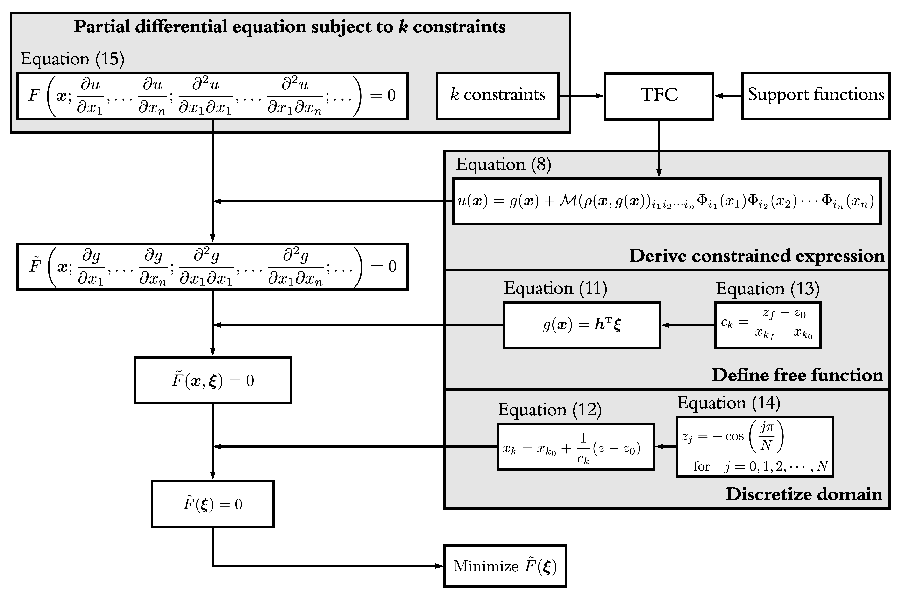
Section 5 discusses how to combine the multivariate constrained expression with multivariate basis functions to estimate the solutions of PDEs. Then, in
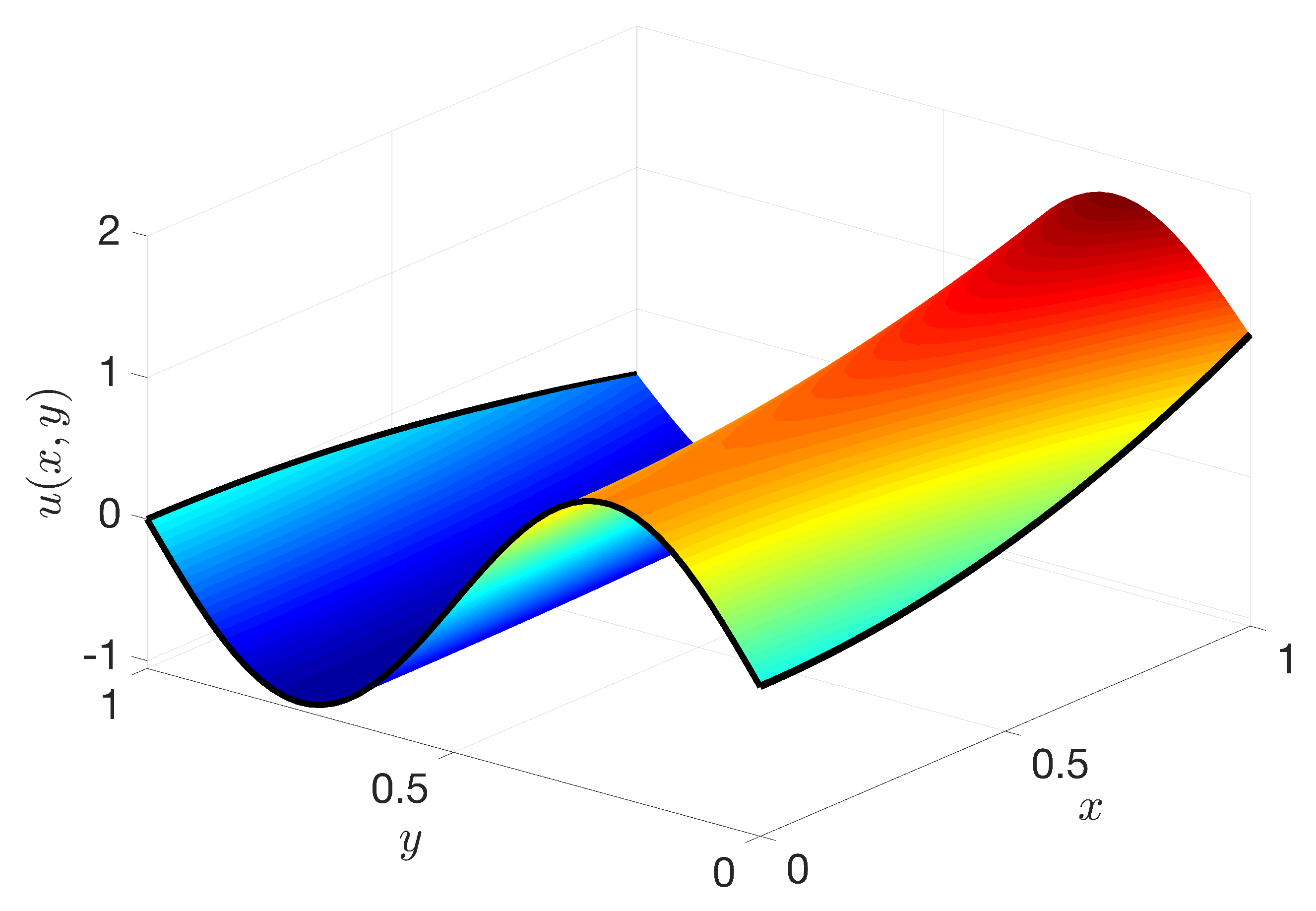
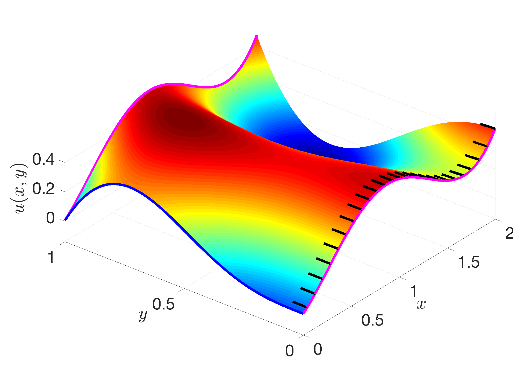
Section 6, this method is used to estimate the solution of two PDEs, and the results are compared with state-of-the-art methods when data is available. Finally,
Section 7 summarizes the article and provides some potential future directions for follow-on research.
3. General Formulation of the Univariate TFC
This section rigorously defines the TFC constrained expression and provides some relevant proofs. First, a functional is defined and its properties are investigated.
Definition 1. A functional, e.g., , has independent variable(s) and function(s) as inputs, and produces a function as an output.
Note that a function as defined here is coincident with the computer science definition of a functional. One can think of a functional as a map for functions. That is, the functional takes a function, , as its input and produces a function, for any specified , as its output. Since this article is focused on constraint embedding, or in other words functional interpolation, we will not concern ourselves with the domain/range of the input and output functions. Rather, we will discuss functionals only in the context of their potential input functions, hereon referred to as the domain of the functional, and potential output functions, hereon referred to as the codomain of the functional.
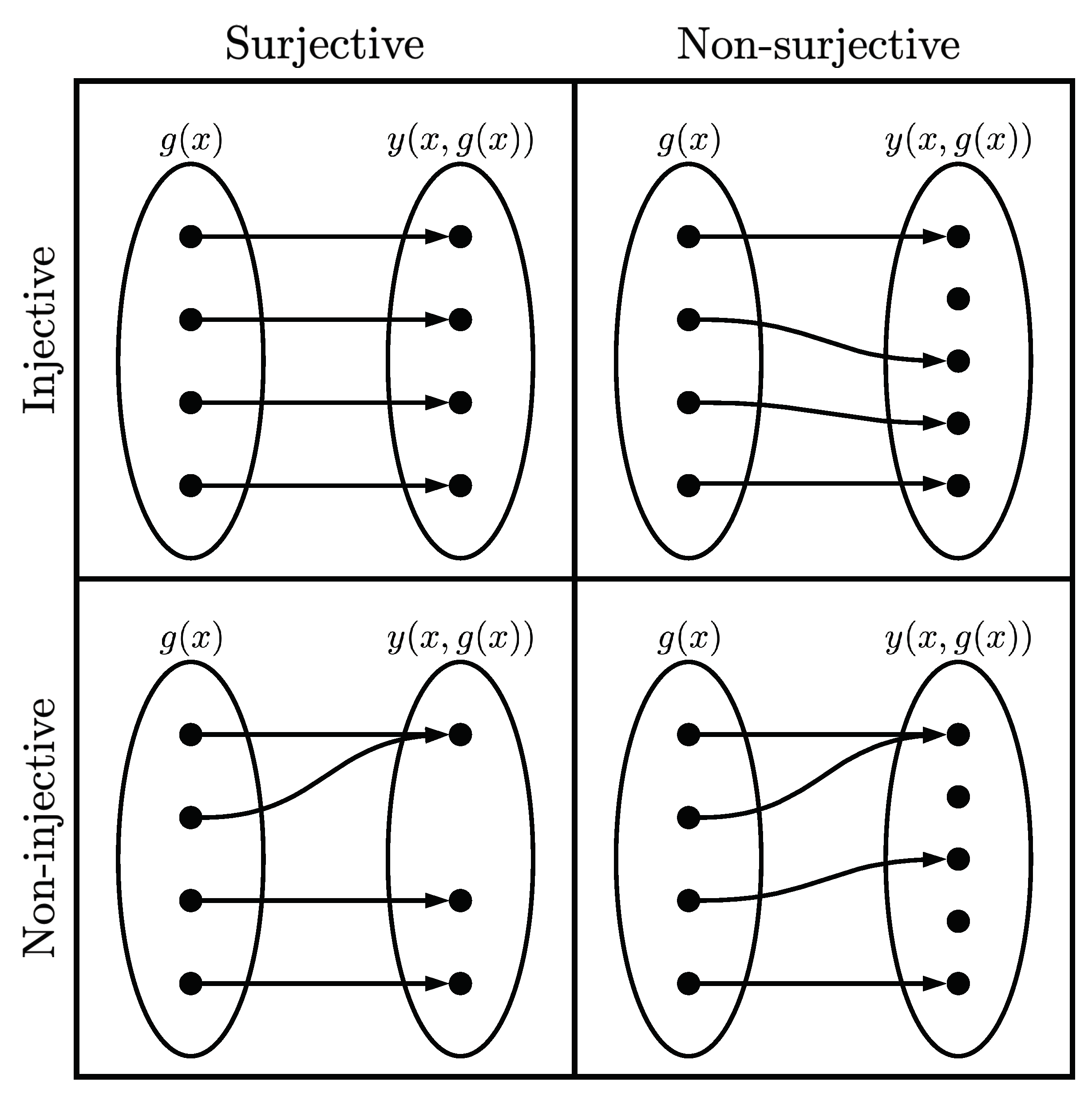
Next, the definitions of injective, surjective, and bijective are extended from functions to functionals.
Definition 2. A functional, , is said to be injective if every function in its codomain is the image of at most one function in its domain.
Definition 3. A functional, , is said to be surjective if for every function in the codomain, , there exists at least one such that .
Definition 4. A functional, , is said to be bijective if it is both injective and surjective.
To elaborate,
Figure 1 gives a graphical representation of each of these functionals, and examples of each of these functionals follow. Note that the phrase “smooth functions” is used here to denote continuous, infinitely differentiable, real valued functions. Consider the functional
whose domain is all smooth functions and whose codomain is all smooth functions. The functional is injective because for every
in the codomain there is at most one
that maps
to
.
However, the functional is not surjective, because the functional does not span the space of the codomain. For example, consider the desired output function : there is no that produces this output. Next, consider the functional whose domain is all smooth functions and whose codomain is the set of all smooth functions such that . This functional is surjective because it spans the space of all smooth functions that are 0 when , but it is not injective. For example, the functions and produce the same result, i.e., . Finally, consider the functional whose domain is all smooth functions and whose codomain is all smooth functions. This functional is bijective, because it is both injective and surjective.
In addition, the notion of projection is extended to functionals. Consider the typical definition of a projection matrix for some . In other words, when P operates on itself, it produces itself: a projection property for functionals can be defined similarly.
Definition 5. A functional is said to be a projection functional if it produces itself when operating on itself.
For example, consider a functional operating on itself, . Then, if , then the functional is a projection functional. Note that proving automatically extends to a functional operating on itself n times: for example, , and so on.
Now that a functional and some properties of a functional have been investigated, the notation used in the prior section can be leveraged to rigorously define TFC related concepts. First, it is useful to define the constraint operator, denoted by the symbol ℭ.
Definition 6. The constraint operator, ℭi, is a linear operator that when operating on a function returns the function evaluated at the i-th specified constraint.
As an example, consider the 2nd linear constraint (
) given in
Section 2.2,
. For this problem, it follows that,
The constraint operator is a linear operator, as it satisfies the two properties of a linear operator: (1)
and (2)
. For example, again consider the 2
linear constraint given in
Section 2.2,
Naturally, the constraint operator has specific properties when operating on the support functions, switching functions, and projection functionals.
Property 3. The constraint operator acting on the support functions produces the matrix Again, consider the example from
Section 2.2 where the support functions were
and
. By applying the constraint operator,
which is identical to the matrix derived in
Section 2.2. In fact, the matrix
is simply the matrix multiplying the
matrix in all the previous examples. Therefore, it follows that,
, where
is the Kroneker delta, and the solution of the
coefficients are precisely the inverse of the constraint operator operating on the support functions.
Property 4. The constraint operator acting on the switching functions produces the Kronecker delta. This property is just a mathematical restatement of the linguistic definition of the switching function given earlier. One can intuit this property from the switching function definition, since they evaluate to 1 at their specified constraint condition (i.e., ) and to 0 at all other constraint conditions (i.e., ).
Using this definition of the constraint operator, one can define the projection functional in a compact and precise manner.
Definition 7. Let be the free function where , and let be the numerical portion of the constraint. Then, Following the example from
Section 2.2, the projection functional for the second constraint is,
Note that in the univariate case
is a scalar value, but in the multivariate case
is a function.
Theorem 1. For any function, , satisfying the constraints, there exists at least one free function, , such that the TFC constrained expression .
Proof. As highlighted in Properties 1 and 2, the projection functionals are equal to zero whenever satisfies the constraints. Thus, if is a function that satisfies the constraints, then the constrained expression becomes . Hence, by choosing , the constrained expression becomes . Therefore, for any function satisfying the constraints, , there exists at least one free function , such that the constrained expression is equal to the function satisfying the constraints, i.e., . □
Theorem 2. The TFC univariate constrained expression is a projection functional.
Proof. To prove Theorem 2, one must show that . By definition, the constrained expression returns a function that satisfies the constraints. In other words, for any , is a function that satisfies the constraints. From Theorem 1, if the free function used in the constrained expression satisfies the constraints, then the constrained expression returns that free function exactly. Hence, if the constrained expression functional is given itself as the free function, it will simply return itself. □
Theorem 3. For a given function, , satisfying the constraints, the free function, , in the TFC constrained expression is not unique. In other words, the TFC constrained expression is a surjective functional.
Proof. Consider the free function choice
where
are scalar values on
and
are the support functions used to construct the switching functions
.
Substituting the chosen
yields,
Now, according to Definition 7 of the projection functional,
Since the constraint operator ℭ
i is a linear operator,
Since
is defined as a function satisfying the constraints, then
, and,
Now, according to Property 3 of the constraint operator, and by decomposing the switching functions
,
Collecting terms results in,
However,
because
is the inverse of
. Therefore, by the definition of inverse,
, and thus,
Simplifying yields the result,
which is independent of the
terms in the free function. Therefore, the free function is not unique. □
Notice that the non-uniqueness of
depends on the support functions used in the constrained expression, which has an immediate consequence when using constrained expressions in optimization. If any terms in
are linearly dependent to the support functions used to construct the constrained expression, their contribution is negated and thus arbitrary. For some optimization techniques it is critical that the linearly dependent terms that do not contribute to the final solution be removed, else, the optimization technique becomes impaired. For example, prior research focused on using this method to solve ODEs [
2,
3] through a basis expansion of
and least-squares, and the basis terms linearly dependent to the support functions had to be omitted from
in order to maintain full rank matrices in the least-squares.
The previous proofs coupled with the functional and functional property definitions given earlier provide a more rigorous definition for the TFC constrained expression: the TFC constrained expression is a surjective, projection functional whose domain is the space of all real-valued functions that are defined at the constraints and whose codomain is the space of all real-valued functions that satisfy the constraints. It is surjective because it spans the space of all functions that satisfy the constraints, its codomain, based on Theorem 1, but is not injective, because Theorem 3 shows that functions in the codomain are the image of more than one function in the domain: the functional is thus not bijective either because it is not injective. Moreover, the TFC constrained expression is a projection functional as shown in Theorem 2.
7. Conclusions
This article illustrated that the structure of the univariate TFC constrained expression is composed of a free function and constraint terms, which contain products of projection functionals and switching functions. A method to calculate the projection functionals and switching functions was demonstrated, and their properties were defined. Then, these properties were used as the foundation for mathematical proofs related to the univariate constrained expression.
In addition, the projection/switching perspective of the univariate constrained expression lead directly to a multivariate extension via recursive application of the univariate theory. Since these multivariate constrained expressions where built from univariate constrained expressions, it was fairly simple to extend the mathematical proofs to the multivariate case as well. In the end, it was concluded that the univariate and multivariate TFC constrained expressions are surjective, projection functionals whose domain is the space of all real-valued functions that are defined at the embedded constraints and whose codomain is the space of all real-valued functions that satisfy said constraints. Additionally, a method for compactly writing multivariate constrained expressions via tensors was provided.
After introducing the multivariate TFC in this way, a methodology for solving PDEs via the TFC was presented. This methodology included choosing the free function to be a linear combination of multivariate orthogonal polynomials, discretizing the domain via collocation points, and finally minimizing the residual of the PDE via least-squares. Two example PDEs solved using this methodology were presented, and when available, the TFC solution accuracy was compared with other state-of-the-art methods.
While this article focused on using orthogonal basis functions, namely, Chebyshev and Legendre orthogonal polynomials, as the free function , and ultimately a linear/nonlinear least-square technique to find the unknown parameters , the technique is not limited to this. At its heart, the TFC approach is a way to derive functionals which analytically satisfy the specified constraints. In other words, when solving ODEs or PDEs, these functionals transform a constrained optimization problem into an unconstrained optimization problem, and therefore a myriad valid definitions of and optimization schemes exist. For example, deep neural networks, support vector machines, and extreme learning machines have been used as free functions in the past. These other free function choices and associated optimization schemes are useful, as for sufficiently complex problems, the number of multivariate basis functions needed to estimate a PDE with sufficient accuracy can become computationally prohibitive.
As defined in this article, the TFC multivariate constrained expressions are capable of embedding value constraints, derivative constraints, and linear combinations thereof. However, other constraint types such as integral, component, and inequality constraints were not discussed. Future work will focus on incorporating these other constraint types. In addition, a more in-depth comparison between TFC and other state-of-the-art methods on a variety of PDEs is likely forthcoming.


