Improving Stability Conditions for Equilibria of SIR Epidemic Model with Delay under Stochastic Perturbations

Abstract

So called SIR epidemic model with distributed delay and stochastic perturbations is considered. It is shown, that the known sufficient conditions of stability in probability of the equilibria of this model, formulated immediately in the terms of the system parameters, can be improved by virtue of the method of Lyapunov functionals construction and the method of Linear Matrix Inequalities (LMIs). It is also shown, that stability can be investigated immediately via numerical simulation of a solution of the considered model.

1. Introduction

Investigation of different versions of the mathematical model of the spread of infections diseases, so called, SIR epidemic models, has a long history, and until now these models are very actual and are very popular in research (see, for instance, [1,2,3,4,5,6,7,8,9,10,11,12,13,14,15,16,17,18,19,20,21,22,23,24,25,26,27,28,29,30]). A big bibliography of SIR epidemic models investigation one can find also in ([31], Ch-11). During its history of development, SIR epidemic models were considered both with constant and distributed delay, both in a deterministic and in a stochastic version. We will consider the SIR epidemic model in the form of the following system of differential equations with distributed delay [2,31]

$$\begin{array}{cc}\hfill \dot{S}\left(t\right)=& b-\beta S\left(t\right){\int }_0^{\infty }I(t-s)dK\left(s\right)-{\mu }_{1}S\left(t\right),\hfill \\ \hfill \dot{I}\left(t\right)=& \beta S\left(t\right){\int }_0^{\infty }I(t-s)dK\left(s\right)-({\mu }_2+\lambda )I\left(t\right),\hfill \\ \hfill \dot{R}\left(t\right)=& \lambda I\left(t\right)-{\mu }_{3}R\left(t\right).\hfill \end{array}$$

(1)

Here, $S\left(t\right)$ is the number of members of a population susceptible to the disease at time t, $I\left(t\right)$ is the number of infective members at time t and $R\left(t\right)$ is the number of members who have been removed from the possibility of infection at time t, through full immunity, b is the recruitment rate of the population, ${\mu }_1$, ${\mu }_2$ and ${\mu }_3$ are the natural death rates of the susceptible, infective and recovered individuals, respectively, $\beta$ is the transmission rate, and $\lambda$ is the natural recovery rate of the infective individuals. The parameters b, $\beta$, $\lambda$, ${\mu }_1$, ${\mu }_2$, ${\mu }_3$ of the system (1) are positive constants, $K\left(s\right)$ is a nondecreasing function, such that

$$\begin{array}{c}{\int }_0^{\infty }dK\left(s\right)=1,\hfill \end{array}$$

(2)

the integrals are understanding in the Stieltjes sense. The equilibria of the system (1) are defined by the conditions $\dot{S}\left(t\right)\equiv 0$, $\dot{I}\left(t\right)\equiv 0$, $\dot{R}\left(t\right)\equiv 0$, i.e., by the system of algebraic equations

$$\begin{array}{c}b=\beta SI+{\mu }_{1}S,\beta SI=({\mu }_2+\lambda )I,\lambda I={\mu }_{3}R,\hfill \end{array}$$

(3)

which has two solutions: $E_0=(b{\mu }_1^{-1},0,0)$ and $E_{+}=(S^{*},I^{*},R^{*})$, where

$$\begin{array}{c}{S}^{*}=\frac{{\mu }_2+\lambda }{\beta }<\frac{b}{{\mu }_1},I^{*}=\frac{b{\left(S^{*}\right)}^{-1}-{\mu }_1}{\beta },R^{*}=\frac{\lambda I^{*}}{{\mu }_3}.\hfill \end{array}$$

(4)

From (4) it follows that $E_{+}$ is a positive equilibrium of the system (1) by the condition

$$\begin{array}{c}b\beta >{\mu }_1({\mu }_2+\lambda ).\hfill \end{array}$$

(5)

Let us suppose that the system (1) is influenced by stochastic perturbations of the white noise type that are directly proportional to the deviation of the system state from the equilibrium $(S^{*},I^{*},R^{*})$. By that the SIR epidemic model (1) under stochastic perturbations is described by the system of Ito’s stochastic differential equations [31,32]

$$\begin{array}{cc}\hfill dS\left(t\right)=& \left(b-\beta S\left(t\right)J\left(I_t\right)-{\mu }_{1}S\left(t\right)\right)dt+{\sigma }_1(S\left(t\right)-S^{*})d{w}_1\left(t\right),\hfill \\ \hfill dI\left(t\right)=& \left(\beta S\left(t\right)J\left(I_t\right)-({\mu }_2+\lambda )I\left(t\right)\right)dt+{\sigma }_2(I\left(t\right)-I^{*})d{w}_2\left(t\right),\hfill \\ \hfill dR\left(t\right)=& \left(\lambda I\left(t\right)-{\mu }_{3}R\left(t\right)\right)dt+{\sigma }_3(R\left(t\right)-R^{*})d{w}_3\left(t\right),\hfill \end{array}$$

(6)

where $w_i\left(t\right)$, $i=1,2,3$, are mutually independent standard Wiener processes [31,32],

$$\begin{array}{c}J\left(I_t\right)={\int }_0^{\infty }I(t-s)dK\left(s\right).\hfill \end{array}$$

(7)

Note that the equilibrium $(S^{*},I^{*},R^{*})$ of the initial deterministic system (1) is the equilibrium of the stochastic system (6) too.

In [31] the following simple sufficient conditions for stability in probability of the equilibria $E_0$ and $E_{+}$ are obtained that are formulated immediately in the terms of the system (6) parameters.

Put ${\delta }_i={\displaystyle \frac{1}{2}}{\sigma }_i^2$, $i=1,2,3$.

Lemma 1.

If

$$\begin{array}{c}{\delta }_1<{\mu }_1,{\delta }_2<{\mu }_2+\lambda -\beta b{\mu }_1^{-1},{\delta }_3<{\mu }_3,\hfill \end{array}$$

(8)

then the equilibrium $E_0$ of the system (6) is stable in probability.

Remark 1.

Note that the second condition (8) contradicts with (5). It means that by the conditions (8) the system (6) does not have the positive equilibrium $E_{+}$.

Lemma 2.

Let be ${\delta }_3<{\mu }_3$ and

$$\begin{array}{c}{\delta }_1<{\mu }_1,{\delta }_2<{\displaystyle \frac{\beta S^{*}\beta I^{*}}{b{\left(S^{*}\right)}^{-1}+\beta S^{*}}}\hfill \end{array}$$

(9)

or

$$\begin{array}{cc}\hfill {\mu }_1\le & {\delta }_1<{\mu }_1+\beta I^{*}{\displaystyle \frac{\sqrt{4I^{*}{\left(S^{*}\right)}^{-1}+1}-1}{\sqrt{4I^{*}{\left(S^{*}\right)}^{-1}+1}+1}},\hfill \\ \hfill {\delta }_2<& {\displaystyle \frac{\beta S^{*}\beta I^{*}}{b{\left(S^{*}\right)}^{-1}+\beta S^{*}}}\left(1-{\displaystyle \frac{\beta S^{*}({\delta }_1-{\mu }_1)}{{(b{\left(S^{*}\right)}^{-1}-{\delta }_1)}^2}}\right).\hfill \end{array}$$

(10)

Then the equilibrium $E_{+}$ of the system (6) is stable in probability.

Below new sufficient conditions for stability in probability of the equilibria $E_0$ and $E_{+}$ are obtained by virtue of the method of Lyapunov functionals construction [31] in the terms of Linear Matrix Inequalities (LMIs) [33] that are essentially less conservative than the conditions (8)–(10).

2. Some Auxiliary Definitions and Statements

Using the new variables $x_1\left(t\right)=S\left(t\right)-S^{*}$, $x_2\left(t\right)=I\left(t\right)-I^{*}$, $x_3\left(t\right)=R\left(t\right)-R^{*}$, transform the system (6) to the form

$$\begin{array}{cc}d{x}_1\left(t\right)=\hfill & (-b{\left(S^{*}\right)}^{-1}{x}_1\left(t\right)-\beta S^{*}J\left(x_{2t}\right)-\beta x_1\left(t\right)J\left(x_{2t}\right))dt+{\sigma }_1{x}_1\left(t\right)d{w}_1\left(t\right),\hfill \\ d{x}_2\left(t\right)=\hfill & (\beta I^{*}{x}_1\left(t\right)-({\mu }_2+\lambda )x_2\left(t\right)+\beta S^{*}J\left(x_{2t}\right)+\beta x_1\left(t\right)J\left(x_{2t}\right))dt+{\sigma }_2{x}_2\left(t\right)d{w}_2\left(t\right),\hfill \\ d{x}_3\left(t\right)=\hfill & (\lambda x_2\left(t\right)-{\mu }_3{x}_3\left(t\right))dt+{\sigma }_3{x}_3\left(t\right)d{w}_3\left(t\right).\hfill \end{array}$$

(11)

It is clear that stability of the equilibrium $(S^{*},I^{*},R^{*})$ of the system (6) is equivalent to stability of the zero solution of the system (11). It is known [31] that for getting sufficient conditions for stability in probability of the zero solution of the nonlinear system (11) it is enough to get sufficient conditions for asymptotic mean square stability of the zero solution of the linear part of this system

$$\begin{array}{cc}d{y}_1\left(t\right)=\hfill & (-b{\left(S^{*}\right)}^{-1}{y}_1\left(t\right)-\beta S^{*}J\left(y_{2t}\right))dt+{\sigma }_1{y}_1\left(t\right)d{w}_1\left(t\right),\hfill \\ d{y}_2\left(t\right)=\hfill & (\beta I^{*}{y}_1\left(t\right)-({\mu }_2+\lambda )y_2\left(t\right)+\beta S^{*}J\left(y_{2t}\right))dt+{\sigma }_2{y}_2\left(t\right)d{w}_2\left(t\right),\hfill \\ d{y}_3\left(t\right)=\hfill & (\lambda y_2\left(t\right)-{\mu }_3{y}_3\left(t\right))dt+{\sigma }_3{y}_3\left(t\right)d{w}_3\left(t\right).\hfill \end{array}$$

(12)

Put $x\left(t\right)={(x_1\left(t\right),x_2\left(t\right),x_3\left(t\right))}^{\prime }$, $y\left(t\right)={(y_1\left(t\right),y_2\left(t\right),y_3\left(t\right))}^{\prime }$.

Definition 1.

The zero solution of the system (11) with the initial condition $x\left(s\right)=\varphi \left(s\right)$, $s\le 0$, is called stable in probability if for any ${\epsilon }_1>0$ and ${\epsilon }_2>0$ there exists $\delta >0$ such that the solution $x(t,\varphi )$ of the system (11) satisfies the condition $\mathbf{P}\{{sup}_{t\ge 0}\left|x(t,\varphi )\right|>{\epsilon }_1\}<{\epsilon }_2$ for any initial function ϕ such that $\mathbf{P}\left\{{sup}_{s\le 0}\right|\varphi \left(s\right)|<\delta \}=1$.

Definition 2.

The zero solution of the system (12) with the initial condition $y\left(s\right)=\varphi \left(s\right)$, $s\le 0$, is called:

-

mean square stable if for each $\epsilon >0$ there exists a $\delta >0$ such that ${\mathbf{E}\left|y(t,\varphi )\right|}^2<\epsilon$, $t\ge 0$, provided that ${\parallel \varphi \parallel }^2={sup}_{s\le 0}\mathbf{E}{\left|\varphi \left(s\right)\right|}^2<\delta$;

-

asymptotically mean square stable if it is mean square stable and for each initial function ϕ the solution $y(t,\varphi )$ of the system (12) satisfies the condition ${lim}_{t\to \infty }\mathbf{E}{\left|y(t,\varphi )\right|}^2=0$;

-

exponentially mean square stable if it is mean square stable and there exists $\lambda >0$ such that for each initial function ϕ there exists $C>0$ (which may depend on ϕ) such that ${\mathbf{E}\left|y(t,\varphi )\right|}^2\le C{e}^{-\lambda t}$ for $t\ge 0$.

Remark 2.

Understanding, that in the neighbourhood of the zero a nonlinear function with the order of nonlinearity higher that one converges to the zero quicker than a linear function, explains why asymptotic mean square stability of the zero solution of the linear part of a nonlinear system guarantees stability in probability of the zero solution of the initial nonlinear system.

Represent the system (12) in the matrix form

$$\begin{array}{cc}\hfill dy\left(t\right)=& \left(Ay\left(t\right)+{\int }_0^{\infty }By(t-s)dK\left(s\right)\right)dt+{\displaystyle \sum _{i=1}^3}{C}_{i}y\left(t\right)d{w}_i\left(t\right),\hfill \end{array}$$

(13)

where the matrix $C_i$ has all zero elements besides of $c_{ii}={\sigma }_i$, $i=1,2,3$,

$$\begin{array}{c}A=\left[\begin{array}{ccc}-b{\left(S^{*}\right)}^{-1}& 0& 0\\ \beta I^{*}& -({\mu }_2+\lambda )& 0\\ 0& \lambda & -{\mu }_3\end{array}\right],B=\left[\begin{array}{ccc}0& -\beta S^{*}& 0\\ 0& \beta S^{*}& 0\\ 0& 0& 0\end{array}\right].\hfill \end{array}$$

(14)

Let $y\left(t\right)$ be a value of the solution of the Equation (13) in the time moment t, $y_t=y(t+s)$, $s<0$, be a trajectory of the solution of the Equation (13) until the time moment t. Consider a functional $V(t,\phi ):[0,\infty )\times H_2\to {\mathbf{R}}_{+}$ that can be presented in the form $V(t,\phi )=V(t,\phi (0),\phi (s\left)\right)$, $s<0$, and for $\phi =y_t$ put

$$V_{\phi }(t,y)=V(t,\phi )=V(t,y_t)=V(t,y,y(t+s)),y=\phi \left(0\right)=y\left(t\right),s<0.$$

(15)

Denote by D the set of the functionals, for which the function $V_{\phi }(t,y)$ defined in (15) has a continuous derivative with respect to t and two continuous derivatives with respect to y. Let ${}^{\prime }$ be the sign of transpose, $\nabla V_{\phi }(t,y)$ and ${\nabla }^2{V}_{\phi }(t,y)$ be, respectively, the vector of the first and the matrix of the second derivatives of the function $V_{\phi }(t,y)$ with respect to y, i.e.,

$$\begin{array}{c}\nabla V_{\phi }(t,y)={\left({\displaystyle \frac{\partial V_{\phi }(t,y)}{\partial y_1}},{\displaystyle \frac{\partial V_{\phi }(t,y)}{\partial y_2}},{\displaystyle \frac{\partial V_{\phi }(t,y)}{\partial y_3}}\right)}^{\prime },{\nabla }^2{V}_{\phi }(t,y)=\left\{{\displaystyle \frac{{\partial }^2{V}_{\phi }(t,y)}{\partial y_i{y}_j}}\right\},i,j=1,2,3.\hfill \end{array}$$

For the functionals from D the generator L of the Equation (13) has the form [31,32]

$$\begin{array}{cc}LV(t,y_t)=\hfill & {\displaystyle \frac{\partial V_{\phi }(t,y\left(t\right))}{\partial t}}+\nabla V_{\phi }^{\prime }(t,y\left(t\right))\left(Ay\left(t\right)+\underset{0}{\overset{\infty }{\int }}By(t-s)dK\left(s\right)\right)\hfill \\ \hfill & +\frac{1}{2}{\displaystyle \sum _{j=1}^3}{y}^{\prime }\left(t\right)C_j^{\prime }{\nabla }^2{V}_{\phi }(t,y\left(t\right))C_{j}y\left(t\right).\hfill \end{array}$$

(16)

Theorem 1.

[31] Let there exist a functional $V(t,\phi )\in D$, positive constants $c_1$, $c_2$, $c_3$, such that the following conditions hold:

$$\mathbf{E}V(t,y_t)\ge c_1\mathbf{E}|y\left(t\right){|}^2,\mathbf{E}V(0,\varphi )\le c_2{\parallel \varphi \parallel }^2,\mathbf{E}LV(t,y_t)\le -c_3\mathbf{E}{\left|y\left(t\right)\right|}^2.$$

(17)

Then the zero solution of the Equation (13) is asymptotically mean square stable.

Lemma 3.

[34] Let $R\in {\mathbf{R}}^{n\times n}$ be a positive definite matrix, $z={\int }_{Q}y\left(s\right)\mu \left(\mathrm{d}s\right)$, where $z,y\left(s\right)\in {\mathbf{R}}^n$, $\mu \left(\mathrm{d}s\right)$ is some measure on Q such that $\mu \left(Q\right)<\infty$ and the integral is defined in the Lebesgue sense. Then

$$z^{\prime }Rz\le \mu \left(Q\right){\int }_Q{y}^{\prime }\left(s\right)Ry\left(s\right)\mu \left(\mathrm{d}s\right).$$

(18)

3. Stability of Equilibria

In this section we obtain sufficient conditions for asymptotic mean square stability of the zero solution of the Equation (13). Via Remark 2 these conditions are also sufficient conditions for stability in probability of the appropriate equilibrium of the system (6).

Below the sign ∗ in a matrix means the symmetric element of a matrix, the inequality A > 0 (A < 0) for a symmetric matrix A means that it is a positive (negative) definite matrix.

3.1. The First Stability Condition

Theorem 2.

Let there exist positive definite $3\times 3$-matrices P and R satisfying the LMI

$$\begin{array}{c}{\Psi }_0=\left[\begin{array}{cc}{\Phi }_0\hfill & PB\\ \ast \hfill & -R\end{array}\right]<0,{\Phi }_0=PA+A^{\prime }P+R+{\displaystyle \sum _{i=1}^3}{C}_i^{\prime }P{C}_i.\hfill \end{array}$$

(19)

Then the equilibrium $(S^{*},I^{*},R^{*})$ of the system (6) is stable in probability.

Proof. 

Let L be the generator of the Equation (13) and $J\left(y_t\right)$ as it defined in (7). Using the general method of Lyapunov functionals construction [31] we will construct the Lyapunov functional for the Equation (13) in the form $V=V_1+V_2$, where $V_1\left(y\left(t\right)\right)=y^{\prime }\left(t\right)Py\left(t\right)$, $P>0$. Via (16) for $V_1\left(y\left(t\right)\right)$ we have

$$\begin{array}{cc}\hfill L{V}_1\left(y\left(t\right)\right)& =2y^{\prime }\left(t\right)P(Ay\left(t\right)+BJ\left(y_t\right))+{\displaystyle \sum _{i=1}^3}{y}^{\prime }\left(t\right)C_i^{\prime }P{C}_{i}y\left(t\right)\hfill \\ & =y^{\prime }\left(t\right)\left(PA+A^{\prime }P+{\displaystyle \sum _{i=1}^3}{C}_i^{\prime }P{C}_i\right)y\left(t\right)+2y^{\prime }\left(t\right)PBJ\left(y_t\right).\hfill \end{array}$$

(20)

Let us choose the additional functional $V_2$ in the form

$$\begin{array}{c}{V}_2(t,y_t)={\int }_0^{\infty }{\int }_{t-s}^t{y}^{\prime }\left(\tau \right)Rz\left(\tau \right)d\tau dK\left(s\right),R>0.\hfill \end{array}$$

Using the inequality (18) and (2), (7), we obtain

$$\begin{array}{c}{J}^{\prime }\left(y_t\right)RJ\left(y_t\right)\le {\int }_0^{\infty }{y}^{\prime }(t-s)Ry(t-s)dK\left(s\right).\hfill \end{array}$$

So, for the functional $V_2$ we have

$$\begin{array}{cc}\hfill L{V}_2(t,y_t)=& y^{\prime }\left(t\right)Ry\left(t\right)-{\int }_0^{\infty }{y}^{\prime }(t-s)Ry(t-s)dK\left(s\right)\hfill \\ \hfill \le & y^{\prime }\left(t\right)Ry\left(t\right)-J^{\prime }\left(y_t\right)RJ\left(y_t\right).\hfill \end{array}$$

(21)

From (20), (21) for the functional $V=V_1+V_2$ it follows that

$$\begin{array}{cc}\hfill LV(t,z_t)\le & z^{\prime }\left(t\right){\Phi }_{0}z\left(t\right)+2y^{\prime }\left(t\right)PBJ\left(y_t\right)-J^{\prime }\left(y_t\right)RJ\left(y_t\right)\hfill \\ \hfill =& \eta \left(t\right){\Psi }_0\eta \left(t\right),\hfill \end{array}$$

(22)

where $\eta \left(t\right)={(y^{\prime }\left(t\right),J^{\prime }\left(y_t\right))}^{\prime }$ and the matrix ${\Psi }_0<0$ is defined in (19). So, the constructed above Lyapunov functional V satisfies the conditions (17) of Theorem 1. Therefore, the zero solution of the Equation (13) is asymptotically mean square stable. The proof is completed. ☐

3.2. The Second Stability Condition

To get the second stability condition note that, using the equality ${\displaystyle \frac{d}{dt}}\left(\underset{0}{\overset{\infty }{\int }}\underset{t-s}{\overset{t}{\int }}z\left(\tau \right)d\tau dK\left(s\right)\right)=z\left(t\right)-\underset{0}{\overset{\infty }{\int }}z(t-s)dK\left(s\right)$, the Equation (13) can be represented in the form of a neutral type equation

$$\begin{array}{c}dZ\left(t\right)=(A+B)z\left(t\right)dt+{\displaystyle \sum _{j=1}^3}{C}_{j}z\left(t\right)d{w}_j\left(t\right),\hfill \\ Z\left(t\right)=z\left(t\right)+G\left(t\right),G\left(t\right)=\underset{0}{\overset{\infty }{\int }}\underset{t-s}{\overset{t}{\int }}Bz\left(\tau \right)d\tau dK\left(s\right).\hfill \end{array}$$

(23)

Remark 3.

For stability investigation of the neutral type Equation (23) it is necessary to ensure the exponential stability of the integral equation $Z\left(t\right)=0$ [35], i.e., via (23)

$$\begin{array}{c}z\left(t\right)=-G\left(t\right).\hfill \end{array}$$

(24)

Similarly to [36,37], it can be shown that if there exists a positive definite matrix $Q\in {\mathbf{R}}^{n\times n}$ such that the LMI

$$\begin{array}{c}{k}_1{B}^{\prime }QB-k_1^{-1}Q<0,k_1={\int }_0^{\infty }sdK\left(s\right),\hfill \end{array}$$

(25)

holds then the integral Equation (24) is exponentially stable.

A simpler, but, generally speaking, more rough than (25) sufficient condition for exponential stability of the integral Equation (24) is the inequality $k_1\parallel B\parallel <1$, where $\parallel B\parallel$ is the matrix norm of a matrix B [31]. Note, however, that in the scalar case $(n=1)$ both these conditions coincide.

Theorem 3.

Let for some positive definite matrices $P,Q,R\in {\mathbf{R}}^{n\times n}$ the LMIs (25) and

$${\Psi }_1=\left[\begin{array}{cc}{\Phi }_1\hfill & {(A+B)}^{\prime }P\\ \ast & -R\end{array}\right]<0,{\Phi }_1={(A+B)}^{\prime }P+P(A+B)+k_1^2{B}^{\prime }RB+{\displaystyle \sum _{j=1}^3}{C}_j^{\prime }P{C}_j,$$

(26)

hold. Then the equilibrium $(S^{*},I^{*},R^{*})$ of the system (6) is stable in probability.

Proof. 

Let L be the generator of the Equation (23). Via (16) and (23) for the functional $V_1\left(z_t\right)=Z^{\prime }\left(t\right)PZ\left(t\right)$, $P>0$, we have

$$\begin{array}{cc}\hfill L{V}_1\left(z_t\right)=& 2Z^{\prime }\left(t\right)P(A+B)z\left(t\right)+{\displaystyle \sum _{j=1}^k}{z}^{\prime }\left(t\right)C_j^{\prime }P{C}_{j}z\left(t\right)\hfill \\ \hfill =& 2z^{\prime }\left(t\right)P(A+B)z\left(t\right)+2G^{\prime }\left(t\right)P(A+B)z\left(t\right)+{\displaystyle \sum _{j=1}^k}{z}^{\prime }\left(t\right)C_j^{\prime }P{C}_{j}z\left(t\right).\hfill \end{array}$$

(27)

From the definition of $G\left(t\right)$ (23) and the inequality (18) it follows that

$$\begin{array}{c}{G}^{\prime }\left(t\right)RG\left(t\right)\le k_1{\int }_0^{\infty }{\int }_{t-s}^t{z}^{\prime }\left(\tau \right)B^{\prime }RBz\left(\tau \right)d\tau dK\left(s\right),k_1={\int }_0^{\infty }sdK\left(s\right).\hfill \end{array}$$

So, for the additional functional

$$\begin{array}{c}{V}_2(t,z_t)=k_1{\int }_0^{\infty }{\int }_{t-s}^t(\tau -t+s)z^{\prime }\left(\tau \right)B^{\prime }RBz\left(\tau \right)d\tau dK\left(s\right)\hfill \end{array}$$

we obtain

$$\begin{array}{cc}\hfill L{V}_2(t,z_t)=& k_1^2{z}^{\prime }\left(t\right)B^{\prime }RBz\left(t\right)-k_1{\int }_0^{\infty }{\int }_{t-s}^t{z}^{\prime }\left(\tau \right)B^{\prime }RBz\left(\tau \right)d\tau dK\left(s\right)\hfill \\ \hfill \le & k_1^2{z}^{\prime }\left(t\right)B^{\prime }RBz\left(t\right)-G^{\prime }\left(t\right)RG\left(t\right).\hfill \end{array}$$

(28)

Via (27), (28) for the functional $V=V_1+V_2$ we have

$$\begin{array}{c}LV(t,z_t)\le z^{\prime }\left(t\right){\Phi }_{1}z\left(t\right)+2G^{\prime }\left(t\right)P(A+B)z\left(t\right)-G^{\prime }\left(t\right)RG\left(t\right)={\eta }^{\prime }\left(t\right){\Psi }_1\eta \left(t\right),\hfill \end{array}$$

(29)

where $\eta \left(t\right)={(z^{\prime }\left(t\right),G^{\prime }\left(t\right))}^{\prime }$ and the matrix ${\Psi }_1<0$ is defined in (26). So, the constructed above Lyapunov functional V satisfies the conditions (17) of Theorem 1. Therefore, the zero solution of the Equation (13) is asymptotically mean square stable. The proof is completed. ☐

3.3. The Third Stability Condition

Let us complement the Equation (23) by the following way

$$\begin{array}{c}dZ\left(t\right)=(A+B)z\left(t\right)dt+{\displaystyle \sum _{j=1}^3}{C}_{j}z\left(t\right)d{w}_j\left(t\right),\hfill \\ dG\left(t\right)=(Bz\left(t\right)-G_0\left(t\right))dt,G_0\left(t\right)={\int }_0^{\infty }Bz(t-s)dK\left(s\right),\hfill \\ Z\left(t\right)=z\left(t\right)+G\left(t\right),G\left(t\right)=\underset{0}{\overset{\infty }{\int }}\underset{t-s}{\overset{t}{\int }}Bz\left(\tau \right)d\tau dK\left(s\right).\hfill \end{array}$$

(30)

Note that for the LMI (19) the matrix A must be the Hurwitz matrix, for the LMI (26) the matrix $A+B$ must be the Hurwitz matrix. Here we also assume that $A+B$ is the Hurwitz matrix. The standard approach to stability analysis of the Equation (30) includes construction of a Lyapunov functional $V\left(x_t\right)$ with the conditions

$$\begin{array}{c}\mathbf{E}V\left(z_t\right)\ge c_1\mathbf{E}|Z\left(t\right){|}^2,\mathbf{E}LV\left(z_t\right)\le -c_2\mathbf{E}{\left|z\left(t\right)\right|}^2,t\ge 0,\hfill \end{array}$$

(31)

that hold for some positive constants $c_1$ and $c_2$, provided the integral equation $Z\left(t\right)=0$ is asymptotically stable [36,37]. In the approach, proposed in this section, similarly to [33,38,39] so called augmented Lyapunov functional $V\left(z_t\right)=V(z_t,G\left(t\right))$ is used, that satisfies to the conditions (17) of the Theorem 1, which is a classical theorem of the type of Lyapunov-Krasovskii. In this case there is no need to verify the stability of the integral equation $Z\left(t\right)=0$.

Theorem 4.

Let there exist $3\times 3$-dimensional matrices $P_1,P_2,P_3,R>0$ and $Q>0$ that satisfy the following LMIs:

$$\begin{array}{c}\Phi =\left[\begin{array}{cc}{P}_1\hfill & P_1+P_2\\ \ast \hfill & P_1+P_2+P_2^{\prime }+P_3+\frac{1}{k_1}Q\end{array}\right]>0\hfill \end{array}$$

(32)

and

$$\begin{array}{c}{\Psi }_2=\left[\begin{array}{ccc}{\Phi }_{11}\hfill & {\Phi }_{12}& P_2\\ *& -R& P_2+P_3\\ *& *& -Q\end{array}\right]<0,\hfill \\ {\Phi }_{11}=P_1(A+B)+{(A+B)}^{\prime }{P}_1+P_{2}B+B^{\prime }{P}_2^{\prime }+B^{\prime }(Q+k_1^{2}R)B+\sum _{j=1}^3{C}_j^{\prime }{P}_1{C}_j,\hfill \\ {\Phi }_{12}=A^{\prime }(P_1+P_2)+B^{\prime }(P_1+P_2+P_2^{\prime }+P_3).\hfill \end{array}$$

(33)

Then the equilibrium $(S^{*},I^{*},R^{*})$ of the system (6) is stable in probability.

Proof. 

Let L be the generator of the Equation (30). Via (30) for the functional

$$V_1\left(z_t\right)={\left[\begin{array}{c}Z\left(t\right)\hfill \\ G\left(t\right)\hfill \end{array}\right]}^{\prime }\left[\begin{array}{cc}{P}_1\hfill & P_2\hfill \\ P_2^{\prime }\hfill & P_3\hfill \end{array}\right] \left[\begin{array}{c}Z\left(t\right)\hfill \\ G\left(t\right)\hfill \end{array}\right]$$

(34)

we have

$$\begin{array}{cc}\hfill L{V}_1\left(z_t\right)=& 2{\left[\begin{array}{c}Z\left(t\right)\hfill \\ G\left(t\right)\hfill \end{array}\right]}^{\prime }\left[\begin{array}{cc}{P}_1\hfill & P_2\hfill \\ P_2^{\prime }\hfill & P_3\hfill \end{array}\right] \left[\begin{array}{c}(A+B)z\left(t\right)\hfill \\ Bz\left(t\right)-G_0\left(t\right)\hfill \end{array}\right]+{\displaystyle \sum _{j=1}^3}{z}^{\prime }\left(t\right)C_j^{\prime }{P}_1{C}_{j}z\left(t\right)\hfill \\ \hfill =& 2{(z\left(t\right)+G\left(t\right))}^{\prime }(P_1(A+B)z\left(t\right)+P_2(Bz\left(t\right)-G_0\left(t\right))\hfill \\ \hfill & +2G^{\prime }\left(t\right)(P_2^{\prime }(A+B)z\left(t\right)+P_3(Bz\left(t\right)-G_0\left(t\right))+{\displaystyle \sum _{j=1}^3}{z}^{\prime }\left(t\right)C_j^{\prime }{P}_1{C}_{j}z\left(t\right)\hfill \\ \hfill =& z^{\prime }\left(t\right)\left[2P_1(A+B)+2P_{2}B+{\displaystyle \sum _{j=1}^3}{C}_j^{\prime }{P}_1{C}_j\right]z\left(t\right)-2z^{\prime }\left(t\right)P_2{G}_0\left(t\right)\hfill \\ \hfill & +2G^{\prime }\left(t\right)[P_1(A+B)+P_{2}B+P_2^{\prime }(A+B)+P_{3}B]z\left(t\right)-2G^{\prime }\left(t\right)(P_2+P_3)G_0\left(t\right)\hfill \\ \hfill =& z^{\prime }\left(t\right)\left[P_{1}A+A^{\prime }{P}_1+(P_1+P_2)B+B^{\prime }(P_1+P_2^{\prime })+{\displaystyle \sum _{j=1}^3}{C}_j^{\prime }{P}_1{C}_j\right]z\left(t\right)-2z^{\prime }\left(t\right)P_2{G}_0\left(t\right)\hfill \\ \hfill & +2z^{\prime }\left(t\right)[A^{\prime }(P_1+P_2)+B^{\prime }(P_1+P_2+P_2^{\prime }+P_3)]G\left(t\right)-2G^{\prime }\left(t\right)(P_2+P_3)G_0\left(t\right).\hfill \end{array}$$

(35)

Using the additional functional

$$\begin{array}{cc}\hfill V_2\left(z_t\right)=& {\int }_0^{\infty }{\int }_{t-s}^t{z}^{\prime }\left(\tau \right)B^{\prime }QBz\left(\tau \right)d\tau dK\left(s\right)\hfill \\ \hfill & +k_1{\int }_0^{\infty }{\int }_{t-s}^t(\tau -t+s)z^{\prime }\left(\tau \right)B^{\prime }RBz\left(\tau \right)d\tau dK\left(s\right)\hfill \end{array}$$

(36)

with $Q,R>0$, we have

$$\begin{array}{cc}\hfill L{V}_2\left(z_t\right)=& z^{\prime }\left(t\right)B^{\prime }QBz\left(t\right)-{\int }_0^{\infty }{z}^{\prime }(t-s)B^{\prime }QBz(t-s)dK\left(s\right)\hfill \\ \hfill & +k_1^2{z}^{\prime }\left(t\right)B^{\prime }RBz\left(t\right)-k_1{\int }_0^{\infty }{\int }_{t-s}^t{z}^{\prime }\left(\tau \right)B^{\prime }RBz\left(\tau \right)d\tau dK\left(s\right).\hfill \end{array}$$

(37)

Via the inequality (18)

$$\begin{array}{cc}\hfill G_0^{\prime }\left(t\right)Q{G}_0\left(t\right)\le & {\int }_0^{\infty }{z}^{\prime }(t-s)B^{\prime }QBz(t-s)dK\left(s\right),\hfill \\ \hfill G^{\prime }\left(t\right)RG\left(t\right)\le & k_1{\int }_0^{\infty }{\int }_{t-s}^t{z}^{\prime }\left(\tau \right)B^{\prime }RBz\left(\tau \right)d\tau dK\left(s\right).\hfill \end{array}$$

(38)

From (37), (38) it follows that

$$\begin{array}{c}L{V}_2\left(z_t\right)\le z^{\prime }\left(t\right)B^{\prime }(Q+k_1^{2}R)Bz\left(t\right)-G_0^{\prime }\left(t\right)Q{G}_0\left(t\right)-G^{\prime }\left(t\right)RG\left(t\right).\hfill \end{array}$$

(39)

As a result for the functional $V\left(z_t\right)=V(z_t,G\left(t\right))=V_1\left(z_t\right)+V_2\left(z_t\right)$ from (35), (39) it follows that $LV\left(z_t\right)\le {\eta }^{\prime }\left(t\right){\Phi }_2\eta \left(t\right)$, where $\eta \left(t\right)=col\{z\left(t\right),G\left(t\right),-G_0\left(t\right)\}$ and ${\Phi }_2<0$ is defined in (33).

Note also that via (34)

$$\begin{array}{cc}\hfill V_1\left(z_t\right)=& {(z\left(t\right)+G\left(t\right))}^{\prime }{P}_1(z\left(t\right)+G\left(t\right))+2{(z\left(t\right)+G\left(t\right))}^{\prime }{P}_{2}G\left(t\right)+G^{\prime }\left(t\right)P_{3}G\left(t\right)\hfill \\ \hfill =& z^{\prime }\left(t\right)P_{1}z\left(t\right)+2z^{\prime }\left(t\right)(P_1+P_2)G\left(t\right)+G^{\prime }\left(t\right)(P_1+P_2+P_2^{\prime }+P_3)G\left(t\right)\hfill \end{array}$$

and via (36), (38)

$$\begin{array}{c}{V}_2\left(z_t\right)\ge {\int }_0^{\infty }{\int }_{t-s}^t{z}^{\prime }\left(\tau \right)B^{\prime }QBz\left(\tau \right)d\tau dK\left(s\right)\ge \frac{1}{k_1}{G}^{\prime }\left(t\right)QG\left(t\right).\hfill \end{array}$$

From this and (32) it follows

$$\begin{array}{c}V\left(z_t\right)\ge {\left[\begin{array}{c}Z\left(t\right)\\ G\left(t\right)\end{array}\right]}^{\prime }\Phi \left[\begin{array}{c}Z\left(t\right)\\ G\left(t\right)\end{array}\right]\ge c_1{\left|z\left(t\right)\right|}^2\hfill \end{array}$$

with $c_1>0$ since $\Phi >0$. Therefore, the constructed functional V satisfies the conditions (17) of Theorem 1 and the zero solution of the system (30) is asymptotically mean square stable. The proof is completed. ☐

Remark 4.

If (26) holds for some $P>0$, $R>0$ then (33) holds for $P_1=P$, $P_2=P_3=0$, the same R and any $Q>0$.

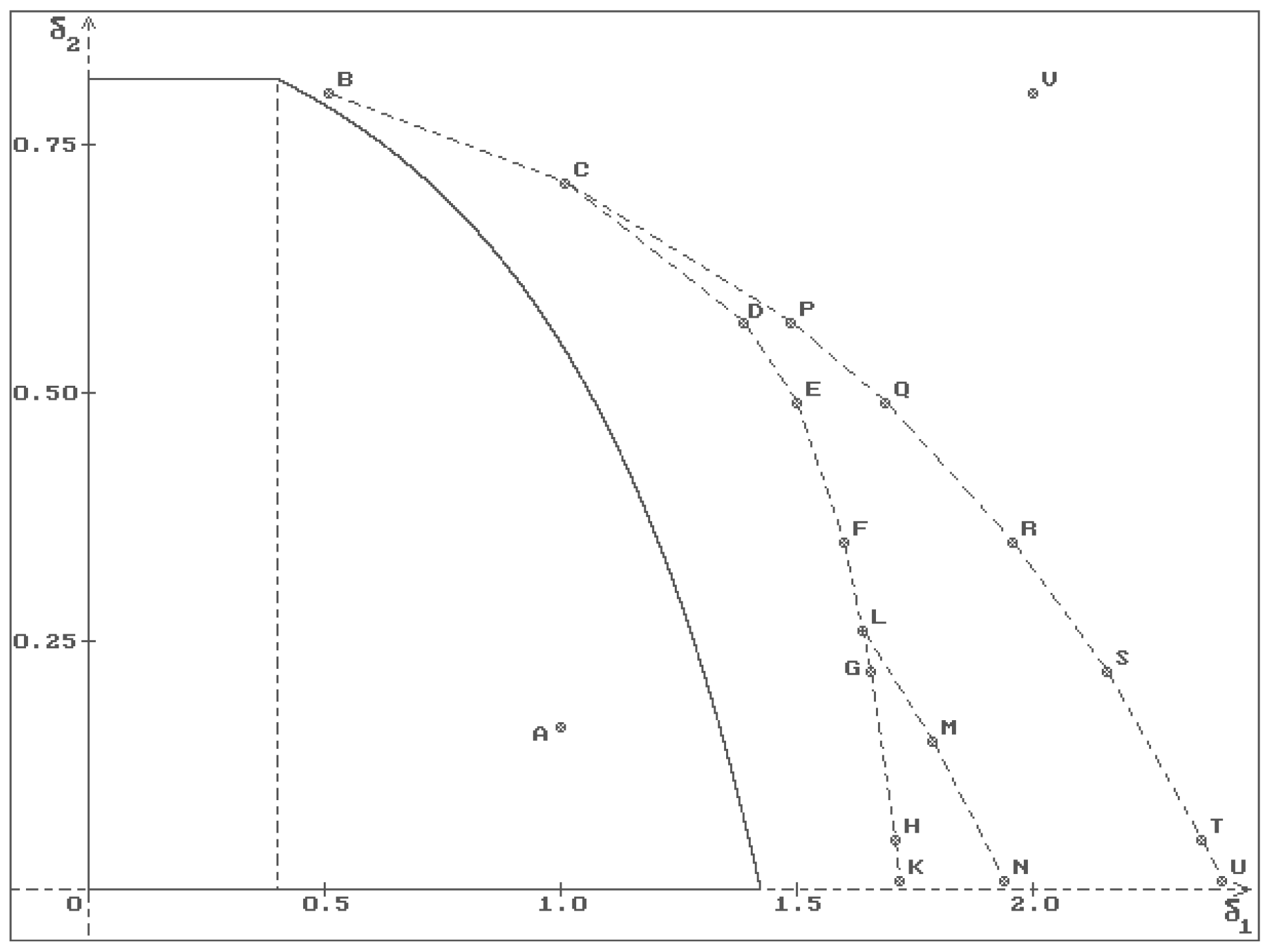
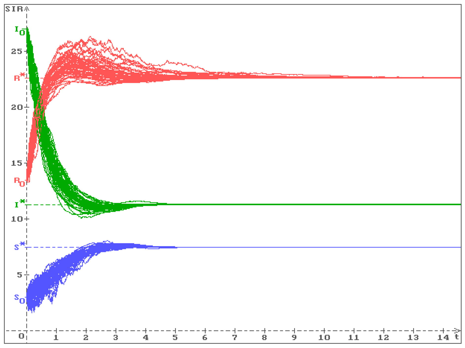
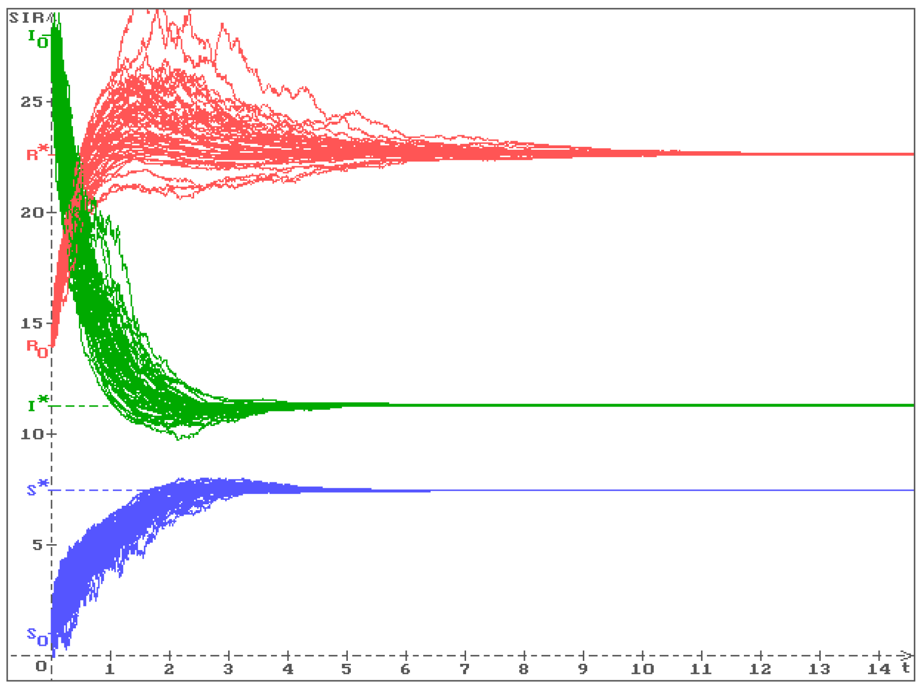
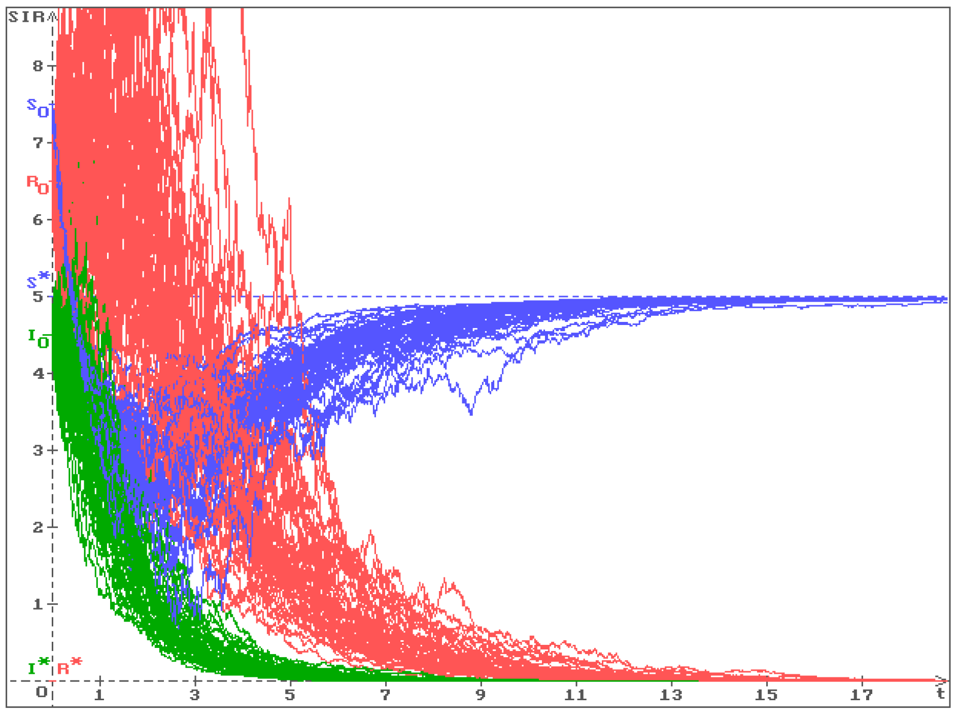
3.4. Numerical Simulations

Suppose that the system (1) has a discrete delay, i.e., $dK\left(s\right)=\delta (s-h)ds$, $h>0$, where $\delta \left(s\right)$ is the Dirac function. So, via (25) $k_1=h$.

Example 1.

Put $b=20$, $\beta =0.2$, $\lambda =1$, ${\mu }_1=0.4$, ${\mu }_2={\mu }_3=0.5$. For these values of the parameters we have via (4) $E_{+}=(S^{*},I^{*},R^{*})=(7.5,11.33,22.67)$. In Figure 1 the stability region of the equilibrium $E_{+}$, that is defined by the conditions (9), (10), is shown (solid line) in the space $({\delta }_1,{\delta }_2)$, ${\delta }_3<{\mu }_3$.

Investigating via MATLAB the LMI (19) with the matrices A and B given in (14) it was shown that the equilibrium $E_{+}=(S^{*},I^{*},R^{*})$ is stable in probability also in the points $B(0.51,0.8)$, $C(1.01,0.71)$, $D(1.39,0.57)$, $E(1.50,0.49)$, $F(1.60,0.35)$, $G(1.66,0.22)$, $H(1.71,0.05)$, $K(1.72,0.01)$.

The LMI (26) more extends the stability region adding the points $L(1.64,0.26)$, $M(1.79,0.15)$, $N(1.94,0.01)$.

At last the LMI (33) makes the stability region much more bigger adding also the points $B(0.51,0.8)$, $C(1.01,0.71)$, $P(1.49,0.57)$, $Q(1.69,0.49)$, $R(1.96,0.35)$, $S(2.16,0.22)$, $T(2.36,0.05)$, $U(2.40,0.01)$.

In Figure 2 50 trajectories of the solution of the SIR epidemic model (6) are shown in the point $A({\delta }_1,{\delta }_2)=A(1,0.16)$ by ${\delta }_3=0.45$, that is placed inside of the stability region defined by (9), (10). One can see that all trajectories with the initial conditions $S\left(0\right)=3$, $I\left(s\right)=27$ for $s\in [-0.1,0]$, $R\left(0\right)=13.5$ converge to the equilibrium $E_{+}=(S^{*},I^{*},R^{*})=(7.5,11.33,22.67)$.

In Figure 3 one can see 50 trajectories of the solution of the SIR epidemic model (6) in the point $Q({\delta }_1,{\delta }_2)=Q(1.69,0.49)$ (see Figure 1) by ${\delta }_3=0.45$. All trajectories with the initial conditions $S\left(0\right)=1$, $I\left(s\right)=28$ for $s\in [-0.1,0]$, $R\left(0\right)=14$ converge to the equilibrium $E_{+}=(S^{*},I^{*},R^{*})=(7.5,11.33,22.67)$.

In Figure 4 50 trajectories of the solution of the SIR epidemic model (6) are shown in the point $V({\delta }_1,{\delta }_2)=V(2,0.8)$ (see Figure 1) by ${\delta }_3=0.7$. All trajectories with the initial conditions $S\left(0\right)=13$, $I\left(s\right)=21$ for $s\in [-0.1,0]$, $R\left(0\right)=17$ converge to the equilibrium $E_{+}=(S^{*},I^{*},R^{*})=(7.5,11.33,22.67)$. Figure 4 shows that the LMIs (19), (26), (33) give sufficient stability conditions only.

Example 2.

Let all values of the parameters be the same as in the Example 1 besides of $b=2$. In this case via (5) the positive equilibrium does not exist and via (8) stability conditions for the equilibrium $E_0=(b{\mu }_1^{-1},0,0)=(5,0,0)$ are ${\delta }_1<0.4$, ${\delta }_2<0.5$, ${\delta }_1<0.5$. Investigating the LMIs (19), (26), (33) with

$$A=\left[\begin{array}{ccc}-{\mu }_1& 0& 0\\ 0& -({\mu }_2+\lambda )& 0\\ 0& \lambda & -{\mu }_3\end{array}\right],B=\left[\begin{array}{ccc}0& -\beta b{\mu }_1^{-1}& 0\\ 0& \beta b{\mu }_1^{-1}& 0\\ 0& 0& 0\end{array}\right],$$

showed that the obtained stability condition (8) does not improve. For instance, for ${\delta }_1=0.39$, ${\delta }_2=0.3$ the LMI (33) holds but for ${\delta }_1=0.4$, ${\delta }_2=0.3$ the LMI (33) does not hold. Similarly to the Example 1, this condition is a sufficient one. In Figure 5 50 trajectories of the solution of the system (6) are shown with the values of the parameters ${\delta }_1=0.39$, ${\delta }_2=0.49$, ${\delta }_3=0.49$, which belong to the obtained stability region. All trajectories with the initial conditions $S\left(0\right)=7.5$, $I\left(s\right)=4.5$, $s\in [-h,0]$, $R\left(0\right)=6.5$ converge to the equilibrium $E_0=(b{\mu }_1^{-1},0,0)=(5,0,0)$. In Figure 6 50 trajectories of the solution of the system (6) are shown with the values of the parameters ${\delta }_1=1.5$, ${\delta }_2=2$, ${\delta }_3=2$, which do not belong to the obtained stability region. It is seen that the effect of stochastic perturbations is stronger than in Figure 5, but all trajectories with the same initial conditions converge to the equilibrium $E_0=(b{\mu }_1^{-1},0,0)=(5,0,0)$ again.

Remark 5.

For numerical simulation of the solution of the SIR epidemic model (6) the algorithm of numerical simulation of trajectories of the Wiener process was used described in [31] and the Euler-Maruyama discretization [31,40,41].

4. Conclusions

On the example of the SIR epidemic model that is very popular in research it is shown how a sequence of stability conditions for equilibria of this model can be obtained in the presence of stochastic perturbations. The method of Lyapunov functionals construction and the method of Linear Matrix Inequalities are used for getting of these stability conditions. Besides it is shown that stability of equilibria can be investigated immediately via numerical simulation of a solution of the considered system. The proposed research can be applied to many other nonlinear mathematical models in different applications, for instance, for social epidemic models: model of alcohol consumption and model of obesity epidemic [31]. From the other hand nobody can say that investigation of the SIR epidemic model can be considered as a complete one. In connection with the current world pandemic it could be interesting and important to establish improving stability conditions for a more realistic SIR epidemic model, which takes into account the death rate and the contact rates where the contact rates depend on the total number of infections; and which under general assumptions, the recovery and death rates then become functions of the total number of infections.

References

1. Ball, F.; Shaw, L. Estimating the within-household infection rate in emerging SIR epidemics among a community of households. J. Math. Biol. 2015, 71, 1705–1735. [Google Scholar] [CrossRef]
2. Beretta, E.; Kolmanovskii, V.; Shaikhet, L. Stability of epidemic model with time delays influenced by stochastic perturbations. Math. Comput. Simul. 1998, 45, 269–277. [Google Scholar] [CrossRef]
3. Beretta, E.; Takeuchi, Y. Global stability of an SIR epidemic model with time delays. J. Math. Biol. 1995, 33, 250–260. [Google Scholar] [CrossRef] [PubMed]
4. Calatayud, J.; Cortes, J.C.; Jornet, M. Computing the density function of complex models with randomness by using polynomial expansions and the RVT technique. Application to the SIR epidemic model. Chaos Solitons Fractals 2020, 133, 109639. [Google Scholar] [CrossRef]
5. Casagrandi, R.; Bolzoni, L.; Levin, S.A.; Andreasen, V. The SIRC model and influenza A. Math. Biosci. 2006, 200, 152–169. [Google Scholar] [CrossRef]
6. Chen, G.; Li, T.; Liu, C. Lyapunov exponent of a stochastic SIR model. C. R. Math. 2013, 351, 33–35. [Google Scholar] [CrossRef]
7. Dieu, N.T.; Nguyen, D.H.; Du, N.H.; Yin, G. Classification of Asymptotic Behavior in a Stochastic SIR Model. SIAM J. Appl. Dyn. Syst. 2016, 15, 1062–1084. [Google Scholar] [CrossRef]
8. Gao, N.; Song, Y.; Wang, X.; Liu, J. Dynamics of a stochastic SIS epidemic model with nonlinear incidence rates. Adv. Differ. Equ. 2019, 2019, 41. [Google Scholar] [CrossRef] [Green Version]
9. Gray, A.; Greenhalgh, D.; Hu, L.; Mao, X.; Pan, J. A stochastic differential equation SIS epidemic model. SIAM J. Appl. Math. 2011, 71, 876–902. [Google Scholar] [CrossRef] [Green Version]
10. Gray, A.; Greenhalgh, D.; Mao, X.; Pan, J. The SIS epidemic model with Markovian switching. J. Math. Anal. Appl. 2012, 394, 496–516. [Google Scholar] [CrossRef] [Green Version]
11. Ji, C.; Jiang, D. Threshold behaviour of a stochastic SIR model. Appl. Math. Model. 2014, 38, 5067–5079. [Google Scholar] [CrossRef]
12. Ji, C.; Jiang, D.; Shi, N. The behavior of an SIR epidemic model with stochastic perturbation. Stoch. Anal. Appl. 2012, 30, 755–773. [Google Scholar] [CrossRef]
13. Jiang, D.; Ji, C.; Shi, N.; Yu, J. The long time behavior of DI SIR epidemic model with stochastic perturbation. J. Math. Anal. Appl. 2010, 372, 162–180. [Google Scholar] [CrossRef] [Green Version]
14. Korobeinikov, A. Global properties of SIR and SEIR epidemic models with multiple parallel infectious stages. Bull. Math. Biol. 2009, 71, 5–83. [Google Scholar] [CrossRef] [PubMed]
15. Korobeinikov, A. Lyapunov functions and global properties for SEIR and SEIS epidemic models. Math. Med. Biol. 2004, 21, 75–83. [Google Scholar] [CrossRef] [PubMed]
16. Kuske, R.; Gordillo, L.; Greenwood, P. Sustained oscillations via coherence resonance in SIR. J. Theor. Biol. 2007, 245, 459–469. [Google Scholar] [CrossRef]
17. Lahrouz, A.; Settati, A. Qualitative Study of a Nonlinear Stochastic SIRS Epidemic System. Stoch. Anal. Appl. 2014, 32, 992–1008. [Google Scholar] [CrossRef]
18. Li, H.; Guo, S. Dynamics of a SIRC epidemiological model. Electron. J. Differ. Equ. 2017, 2017, 1–18. [Google Scholar]
19. Liu, M.; Bai, C.; Wang, K. Asymptotic stability of a two-group stochastic SEIR model with infinite delays. Commun. Nonlinear Sci. Numer. Simul. 2014, 19, 3444–3453. [Google Scholar] [CrossRef]
20. Liu, Q.; Jiang, D.; Hayat, T.; Ahmad, B. Analysis of a delayed vaccinated SIR epidemic model with temporary immunity and Levy jumps. Nonlinear Anal. Hybrid Syst. 2018, 27, 29–43. [Google Scholar] [CrossRef]
21. Liu, Q.; Jiang, D.; Shi, N.; Hayat, T.; Alsaedi, A. Stationary distribution and extinction of a stochastic SIRS epidemic model with standard incidence. Phys. A Stat. Mech. Appl. 2017, 469, 510–517. [Google Scholar] [CrossRef]
22. Lu, Q. Stability of SIR system with random perturbations. Phys. A Stat. Mech. Appl. 2009, 388, 3677–3686. [Google Scholar] [CrossRef]
23. Miao, A.; Zhang, T.; Zhang, J.; Wang, C. Dynamics of a stochastic SIR model with both horizontal and vertical transmission. J. Appl. Anal. Comput. 2018, 8, 1108–1121. [Google Scholar]
24. Song, Y.; Miao, A.; Zhang, T.; Wang, X.; Liu, J. Extinction and persistence of a stochastic SIRS epidemic model with saturated incidence rate and transfer from infectious to susceptible. Adv. Differ. Equ. 2018, 2018, 293. [Google Scholar] [CrossRef] [Green Version]
25. Tornatore, E.; Buccellato, S.M. On a stochastic SIR model. Appl. Math. 2007, 34, 389–400. [Google Scholar] [CrossRef]
26. Tuckwell, H.C.; Williams, R.J. Some properties of a simple stochastic epidemic model of SIR type. Math. Biosci. 2007, 208, 76–97. [Google Scholar] [CrossRef]
27. Vlasic, A.; Troy, D. Modeling stochastic anomalies in an SIS system. Stoch. Anal. Appl. 2017, 35, 27–39. [Google Scholar] [CrossRef]
28. Yang, Y.; Zhang, T.; Xu, Y. Dynamical analysis of a diffusive SIRs model with general incidence rate. Discret. Contin. Dyn. Syst. Ser. B 2020, 25, 2433–2451. [Google Scholar] [CrossRef] [Green Version]
29. Zhao, Y.; Zhang, L.; Yuan, S. The effect of media coverage on threshold dynamics for a stochastic SIS epidemic model. Phys. A Stat. Mech. Appl. 2018, 512, 248–260. [Google Scholar] [CrossRef]
30. Zhou, Y.; Yuan, S.; Zhao, D. Threshold behavior of a stochastic SIS model with jumps. Appl. Math. Comput. 2016, 275, 255–267. [Google Scholar]
31. Shaikhet, L. Lyapunov Functionals and Stability of Stochastic Functional Differential Equations; Springer Science & Business Media: Berlin, Germany, 2013. [Google Scholar]
32. Gikhman, I.I.; Skorokhod, A.V. Stochastic Differential Equations; Springer: Berlin, Germany, 1972. [Google Scholar]
33. Fridman, E.; Shaikhet, L. Simple LMIs for stability of stochastic systems with delay term given by Stieltjes integral or with stabilizing delay. Syst. Control Lett. 2019, 124, 83–91. [Google Scholar] [CrossRef]
34. Burgos, C.; Cortes, J.C.; Shaikhet, L.; Villanueva, R.J. A nonlinear dynamic age-structured model of e-commerce in Spain: Stability analysis of the equilibrium by delay and stochastic perturbations. Commun. Nonlinear Sci. Numer. Simul. 2018, 64, 149–158. [Google Scholar] [CrossRef]
35. Hale, J.K.; Verduyn Lunel, S.M. Introduction to Functional Differential Equations; Springer: New York, NY, USA, 1993. [Google Scholar]
36. Fridman, E.; Shaikhet, L. Delay-induced stability of vector second-order systems via simple Lyapunov functionals. Automatica 2016, 74, 288–296. [Google Scholar] [CrossRef]
37. Melchor-Aguilar, D.; Kharitonov, V.I.; Lozano, R. Stability conditions for integral delay systems. Int. J. Robust Nonlinear Control 2010, 20, 1–15. [Google Scholar] [CrossRef]
38. Li, Z.Y.; Lam, J.; Wang, J. Stability analysis of linear stochastic neutral-type time-delay systems with two delays. Automatica 2018, 91, 179–189. [Google Scholar] [CrossRef]
39. Seuret, A.; Gouaisbaut, F.; Ariba, Y. Complete quadratic Lyapunov functionals for distributed delay systems. Automatica 2015, 62, 168–176. [Google Scholar] [CrossRef] [Green Version]
40. Liu, L.; Li, M.; Deng, F. Stability equivalence between the neutral delayed stochastic differential equations and the Euler-Maruyama numerical scheme. Appl. Numer. Math. 2018, 127, 370–386. [Google Scholar] [CrossRef]
41. Pang, S.; Deng, F.; Mao, X. Almost sure and moment exponential stability of Euler-Maruyama discretizations for hybrid stochastic differential equations. J. Comput. Appl. Math. 2008, 213, 127–141. [Google Scholar] [CrossRef] [Green Version]
Figure 1. Stability region for the equilibrium E + = S * , I * , R * of the system (6) defined by (9), (10) (solid line) and stability points obtained via LMI (19) (B-K), LMI (26) (L-N) and LMI (33) (B-U).
Mathematics 08 01302 g001
Figure 2. 50 trajectories of the solution of the system (6): S ( t ) (blue), I ( t ) (green), R ( t ) (red) with the initial values S ( 0 ) = 3 , I ( s ) = 27 , s [ h , 0 ] , R ( 0 ) = 13.5 in the point A ( δ 1 , δ 2 ) = A ( 1 , 0.16 ) , δ 3 = 0.45 , h = 0.1 .
Mathematics 08 01302 g002
Figure 3. Fifty trajectories of the solution of the system (6) solution: S ( t ) (blue), I ( t ) (green), R ( t ) (red) with the initial values S ( 0 ) = 1 , I ( s ) = 28 , s [ h , 0 ] , R ( 0 ) = 14 in the point Q ( δ 1 , δ 2 ) = Q ( 1.69 , 0.49 ) , δ 3 = 0.45 , h = 0.1 .
Mathematics 08 01302 g003
Figure 4. Fifty trajectories of the solution of the system (6) solution: S ( t ) (blue), I ( t ) (green), R ( t ) (red) with the initial values S ( 0 ) = 13 , I ( s ) = 21 , s [ h , 0 ] , R ( 0 ) = 17 in the point V ( δ 1 , δ 2 ) = V ( 2 , 0.8 ) , δ 3 = 0.7 , h = 0.1 .
Mathematics 08 01302 g004
Figure 5. Fifty trajectories of the solution of the system (6) solution: S ( t ) (blue), I ( t ) (green), R ( t ) (red) with the initial values S ( 0 ) = 7.5 , I ( s ) = 4.5 , s [ h , 0 ] , R ( 0 ) = 6.5 and δ 1 = 0.39 , δ 2 = 0.49 , δ 3 = 0.49 , h = 0.1 .
Mathematics 08 01302 g005
Figure 6. Fifty trajectories of the solution of the system (6) solution: S ( t ) (blue), I ( t ) (green), R ( t ) (red) with the initial values S ( 0 ) = 7.5 , I ( s ) = 4.5 , s [ h , 0 ] , R ( 0 ) = 6.5 and δ 1 = 1.5 , δ 2 = 2 , δ 3 = 2 , h = 0.1 .
Mathematics 08 01302 g006