Article

Cokriging Prediction Using as Secondary Variable a Functional Random Field with Application in Environmental Pollution

1
Department of Statistics, Universidad Nacional de Colombia, Bogotá 111321, Colombia
2
School of Industrial Engineering, Pontificia Universidad Católica de Valparaíso, Valparaíso 2362807, Chile
*
Author to whom correspondence should be addressed.
Mathematics 2020, 8(8), 1305; https://doi.org/10.3390/math8081305
Submission received: 16 July 2020 / Revised: 3 August 2020 / Accepted: 4 August 2020 / Published: 6 August 2020
(This article belongs to the Special Issue Statistical Simulation and Computation)

Abstract

:
Cokriging is a geostatistical technique that is used for spatial prediction when realizations of a random field are available. If a secondary variable is cross-correlated with the primary variable, both variables may be employed for prediction by means of cokriging. In this work, we propose a predictive model that is based on cokriging when the secondary variable is functional. As in the ordinary cokriging, a co-regionalized linear model is needed in order to estimate the corresponding auto-correlations and cross-correlations. The proposed model is utilized for predicting the environmental pollution of particulate matter when considering wind speed curves as functional secondary variable.

1. Introduction and Bibliographical Review

Geostatistics is a branch of statistics used for performing spatial prediction when realizations of univariate or multivariate random fields are available [1]. Kriging, cokriging, and multivariate kriging are some techniques that are used for prediction in geostatistics (also known as spatial statistics) [2]. These techniques are generalized forms of univariate and multivariate linear regression models based on georeferenced data, which often have spatial dependence. Those interested in an overview about these techniques, and spatial statistics in general, are referred to [1,2,3,4].
Geostatistics is used in many different areas, such as ecology, geology, meteorology, and mining. In some applications of these areas, multiple variables are measured at each location of the region of interest. For example, in environmental studies, often data of several air pollutants, such as carbon monoxide (CO), ozone (O3), and particulate matter (PM), are collected at each monitoring station. Air quality can be evaluated in terms of concentrations of PM with diameter smaller than 10 mm (PM10) [5,6,7,8,9,10]. These pollutants may be correlated and then using all observed variables may improve the prediction [11].
Cokriging is a generalization of the kriging technique. Cokriging has been developed in order to deal with multivariate spatial interpolation (prediction) [12,13]. The cokriging technique has been widely studied and adapted to different practical scenarios. This technique is used to take advantage of the covariance between two or more realizations of cross-correlated random fields. Some variations of cokriging are the ordinary kriging [14], universal kriging [15], collocated kriging [16], and indicator kriging [17]. In the cokriging technique, information of one or more secondary variables is used for reducing the prediction variance of the primary variable. It has been demonstrated that cokriging is better than kriging in terms of the costs and precision of the predictions, when the random fields under study are cross-correlated [18].
Nowadays, the geostatistical prediction techniques (kriging and cokriging) have been extended to deal with realizations of functional random fields [19]. This is a relatively new research area, called functional geostatistics [20,21].
The first attempt to apply geostatistical interpolation techniques in the prediction of unvisited sites was done in the pioneering work that was published in [22]. Later, several kriging predictors for stationary [23,24,25] and non-stationary [26,27,28] functional random fields have been proposed. In such proposals, a spatial prediction of a functional variable was performed. In the case of stationarity, only the realization of the underlying functional random field is considered. However, in the non-stationary case, scalar covariates (for example, altitude, latitude, or longitude) or functional covariates can be used to estimate the trend. In the methodologies proposed in [20,23] for predicting functional variables, a preliminary step using basis functions is considered. After expanding in terms of basis functions, geostatistical prediction of functional variables becomes an ordinary cokriging prediction, which consists of cokriging on the estimated coefficients.
Note that cokriging can be used to predict both a scalar variable (using data of a multivariate random field) or a functional variable (when data of a functional random field are studied and the curves are represented by basis functions). In many areas, and particularly in environmental sciences, it is common to obtain simultaneously spatial data of scalar and functional variables. For instance, data of annual precipitation and average monthly temperature profiles were analyzed in [29], which were collected at 35 weather stations from Canada. Thus, when data of scalar and functional variables for several sites of a region are available, it could be of interest to perform spatial prediction by using all available data. To the best of our knowledge, no studies on cokriging prediction using a functional random field, as secondary variable, have been considered in the literature to date.
From the perspective of the empirical application of our work, note that the relation between PM10 and wind speed (WS) has been widely studied. For example, a forecasting model was formulated in [30] for the daily average PM10 using as input temperature, cloud cover, wind direction, and WS. Similarly, a model was proposed in [31], where temperature, relative humidity and WS were used as covariates. As a general rule, PM10 concentrations decrease as WS increases, but this is not always the case. For example, a direct relationship between these variables was found in the Kathmandu valley [32]. All of the above-mentioned studies evaluated the relationship between PM10 and WS by using scalar data of both variables. Therefore, to the best of our knowledge, no empirical studies relating PM10 and WS curves (functional data) by means of a spatial or co-regionalized linear model (CLM) have been considered until now. An overview about the CLM and some algorithms to find out co-regionalization matrices is given in [33,34].
Therefore, the objectives of this paper are twofold. The main objective is to propose a cokriging predictor of a scalar primary variable considering, as secondary variable, the realization of a functional random field. The secondary objective is to apply our methodology for relating PM10 and WS curves by using a CLM. The proposed cokriging predictor has a similar expression to the ordinary cokriging predictor employed in multivariate geostatistics. However, the secondary variable is now given by the coefficients obtained after representing the functional data in terms of basis functions. As in the ordinary scenario, a CLM is utilized to estimate the auto-correlation and cross-correlations functions required for estimating the corresponding parameters. The empirical application is based on real data to predict PM10 using a functional WS in Bogotá city, Colombia, one of the places with the worst air quality around the world [35].
The paper is organized, as follows. Section 2 gives an overview about cokriging prediction and introduces the cokriging technique based on scalar and functional variables. In Section 3, we use the methodology that was proposed for performing spatial prediction of the primary variable PM10 using curves of WS as secondary variable. The article ends with Section 4 providing conclusions, discussion, and suggestions for further research. Some detailed mathematical expressions are presented in the Appendix A.

2. Cokriging Using as Secondary Variable a Functional Random Field

In this section, we provide background of the ordinary cokriging predictor [36,37]. Subsequently, we outline the procedure to perform cokriging prediction based on a functional secondary variable. An expression for the predictor is deduced as a natural extension of the ordinary cokriging predictor when secondary variables are considered. Hence, we show how using basis functions to expand the functional variable allows us to come back to an ordinary scenario where the estimation procedure is known.

2.1. Ordinary Cokriging Predictor

A generalization of kriging prediction can be obtained when, instead of one stochastic process, we consider realizations of m random fields. Let ( X 1 ( s ) , , X m ( s ) ) be a multivariate spatial vector of m random fields on a region D R d . Here, we assume that the m processes are stationary, which means that the mean vector is assumed to be constant for all s D , and the covariance and variogram functions only depend on the distance vector and not on the location s .
Let X 1 ( s ) be the primary variable and X j ( s ) , for  j = 2 , , m , the secondary variables. The cokriging predictor of X 1 ( s ) in the location s 0 is given by [36]
X ^ 1 ( s 0 ) = i = 1 n λ i X 1 ( s i ) + i = 1 n α i 2 X 2 ( s i ) + + i = 1 n α i m X m ( s i ) = i = 1 n λ i X 1 ( s i ) + i = 1 n j = 2 m α i j X j ( s i ) .
Observe that the predictor defined in (1) is unbiased if i = 1 n λ i = 1 and i = 1 n α i j = 0 .
We use the following notations:
(i)
2 γ l q ( s i , s j ) = Cov ( X l ( s i ) X q ( s j ) ) , for  l , q = 1 , , m .
(ii)
γ l q = ( γ l q ( s 1 , s 0 ) , , γ l q ( s n , s 0 ) ) .
(iii)
Γ l q = γ l q ( s 1 , s 1 ) γ l q ( s 1 , s n ) γ l q ( s n , s 1 ) γ l q ( s n , s n ) .
By using the method of Lagrange multipliers, the cokriging system of equations must be solved in order to minimize the mean squared prediction error subject to the unbiasedness constraints [36]; see its matrix representation in the Appendix A. As usual in multivariable geostatistics, the solution to the system of equations above-mentioned and given in (A1) of the Appendix A is computed by fitting a CLM.

2.2. Cokriging Predictor Using Functional Secondary Variables

Now, suppose that the number of secondary variables is very large. Then, they can be replaced by a functional variable in order to define the cokriging predictor by using secondary variables of a random field. Subsequently, by employing the same idea given in [29] when the functional linear model for scalar response is introduced, suppose in (1) that m . Thus, the parameters α i j defined in (1) can be replaced by a function α i ( t ) , whereas the secondary variables X 2 ( s i ) , , X m ( s i ) may be replaced by a functional variable X s i ( t ) . Therefore, the cokriging predictor of X 1 ( s ) in the location s 0 takes now the form
X ^ 1 ( s 0 ) = i = 1 n λ i X 1 ( s i ) + i = 1 n T α i ( t ) X s i ( t ) d t ,
where X ^ 1 ( s 0 ) is the prediction of the primary variable at an unsampled site s 0 , λ i provides the effect of the scalar variable X 1 ( s i ) on the prediction, X s i ( t ) is a functional variable at the site s i , and  α i ( t ) is a functional parameter, which gives the weight of X s i ( t ) on the prediction, for  i = 1 , , n .
We employ an approach based on basis functions of B-splines and Fourier type in order to perform the parameter estimation [29]. We expand the functional variables and parameters, respectively, by 
X s i ( t ) = j = 1 k a i j ϕ j ( t ) = a i ϕ ( t ) ,
α i ( t ) = j = 1 k α i j ϕ j ( t ) = α i ϕ ( t ) ,
where ϕ ( t ) = ( ϕ 1 ( t ) , , ϕ k ( t ) ) is the vector of basis functions and α i , a i are vectors of estimated coefficients, which are obtained by least squares [29]. By using basis functions and the expansions of the functional variables and parameters that are defined in (3) and (4), respectively, the predictor stated in (1) and (2) is now given by
X ^ 1 ( s 0 ) = i = 1 n λ i X 1 ( s i ) + i = 1 n α i T ϕ ( t ) ϕ ( t ) d t a i = i = 1 n λ i X 1 ( s i ) + i = 1 n α i W a i = i = 1 n λ i X 1 ( s i ) + i = 1 n α i a i * = i = 1 n λ i X 1 ( s i ) + i = 1 n j = 1 k α i j a i j * ,
where α i j are defined in (4) and
a i * = a i 1 * , , a i j * , , a i k * .
Details of the vector a i * are provided in (A2) of the Appendix A.
Remark 1.
A particular case of the predictor given in (5) is obtained when a i j * = a i j . This occurs when orthonormal basis functions, such as Fourier basis, are used. The predictor that is proposed in (5) is similar to the ordinary cokriging predictor stated in (1), but considering coefficients of basis functions instead of variables. Once the coefficients a i j * defined in (6) are calculated, we have a cokriging prediction as in the ordinary case and then the theory above described may be used. A detailed review on multivariate geostatistics, and particularly on the cokriging technique, is presented in [3].

3. Real Data Analysis

In this section, we predict PM10 in Bogotá with our methodology. First, we define the problem upon study and then the cokriging prediction for PM10 is performed using WS curves.

3.1. Definition of the Problem upon Study

Air pollution can be assessed by means of concentrations of PM10 (in μ / g 3 ) [6,8]. The inhalation of PM is known to lead to serious health problems [5,10,30]. These particles are small enough to penetrate the respiratory tract of humans and for this reason they are potential disrupter of the normal functioning of the organism [31]. It is evident that having a model that is capable of predicting the maximum of PM10 in unmonitored areas of a city can be useful to environmental institutions in order to alert, when necessary, the population that is exposed at risk. We use the methodology proposed in this work to perform spatial prediction of maximum PM10 in Bogotá city based on data of this variable and WS data.
The data upon analysis were collected in ten stations from the air quality monitoring network in Bogotá city; see Figure 1. For each station, a maximum PM10 value is obtained; see Table 1. The maximum values were calculated from data that were collected hourly between 26 January 2011 (12:00 p.m.) and 3 February 2011 (2:00 p.m.). The bubble map of Figure 1 shows that the highest PM10 values are collected in the south-western part of the city (Kennedy and Carvajal stations). This is an expected result, because such stations are located in industrial zones [35]. The bubble map also indicates that stations in central and north-east zones of the city (such as IDRD, Ferias, Usaquen) have the lowest values, possibly because they have wetlands and urban woodlands around [35].
As mentioned in the introduction of this paper, the relation between WS and PM10 has been widely analyzed, but all of the mentioned studies evaluated the relationship using scalar data of both variables. In the present application, we consider a different approach, where the temporal variation of WS (a curve considered as functional data) is used for predicting a scalar variable (corresponding to the maximum PM10 in a period of eight days).
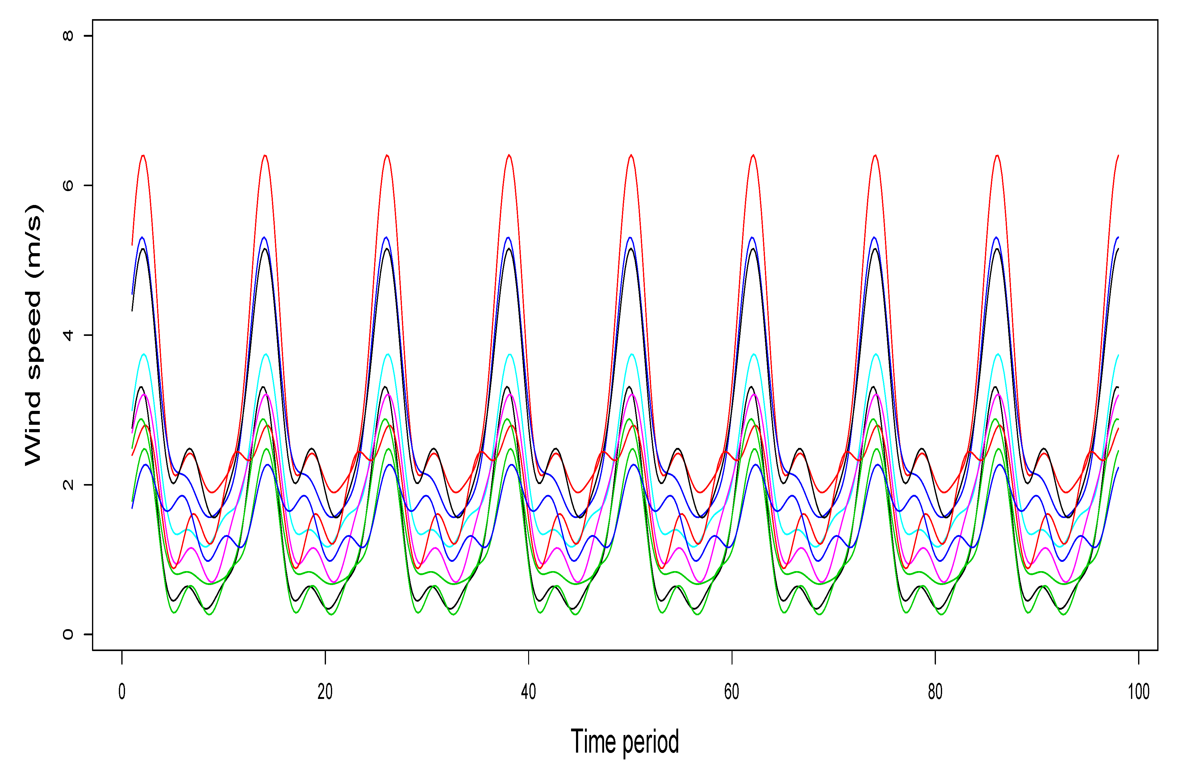
The data of WS (in m/s) at each station were collected each two hours between 26 January 2011 (10:00 a.m.) and 3 February 2011 (12:00 p.m.). In total, we have a WS data set of 98 observations at each monitoring station displayed in Figure 2. Two aspects can be highlighted from the temporal pattern of the WS data. The time-series have their highest peaks at 12:00 p.m. and three stations have significantly higher values than the others (curves in red, black, and dark blue in Figure 2). These values correspond to Fontibon, Kennedy, and Puente Aranda stations; see bubble map of Figure 1.
From Table 1, note that two of the highest PM10 values are obtained at stations that have high WS peaks (Kennedy and Puente Aranda). As mentioned, although it is not usual, some studies have reported direct correlation between the PM10 and WS variables.

3.2. Cokriging Prediction of PM10 Using WS Curves

There are several options for smoothing time series by using basis functions. Frequently, B-splines and Fourier basis are considered [29]. The second option is applied when a seasonal variation is present [29]. Given that time series show a periodic pattern in Figure 2, we consider a Fourier basis of dimension k = 7 (estimated by cross-validation [29]) for smoothing the data. Table 1 provides the estimated coefficients of this basis. The obtained WS curves are shown in Figure 3, from where the pattern described above with the original data is more clearly observed in this figure. There are three stations with higher WS magnitudes than the remaining (red, black, and blue lines).
In summary, for each monitoring station, we dispose of a PM10 value and seven coefficients (resulting from fitting a Fourier basis to WS data) that characterize the information that is given by the curves. The functional data are now represented by the seven coefficients. As mentioned, now a complex spatial problem in which a functional covariate is considered becomes a classical problem with scalar covariates that can be solved by means of an ordinary cokriging technique.
First, a CLM was fitted based on the data reported in Table 1. A Gaussian model [14] was considered for describing all simple and cross variograms. The R software was used for obtaining the calculations [38] and an R package named gstat [39] was used to estimate the corresponding parameters. The data and R codes used in this empirical application are available at [40]. The estimated range of simple and cross-variograms was 8 km (about one-third of the maximum distance between monitoring sites in Figure 1).
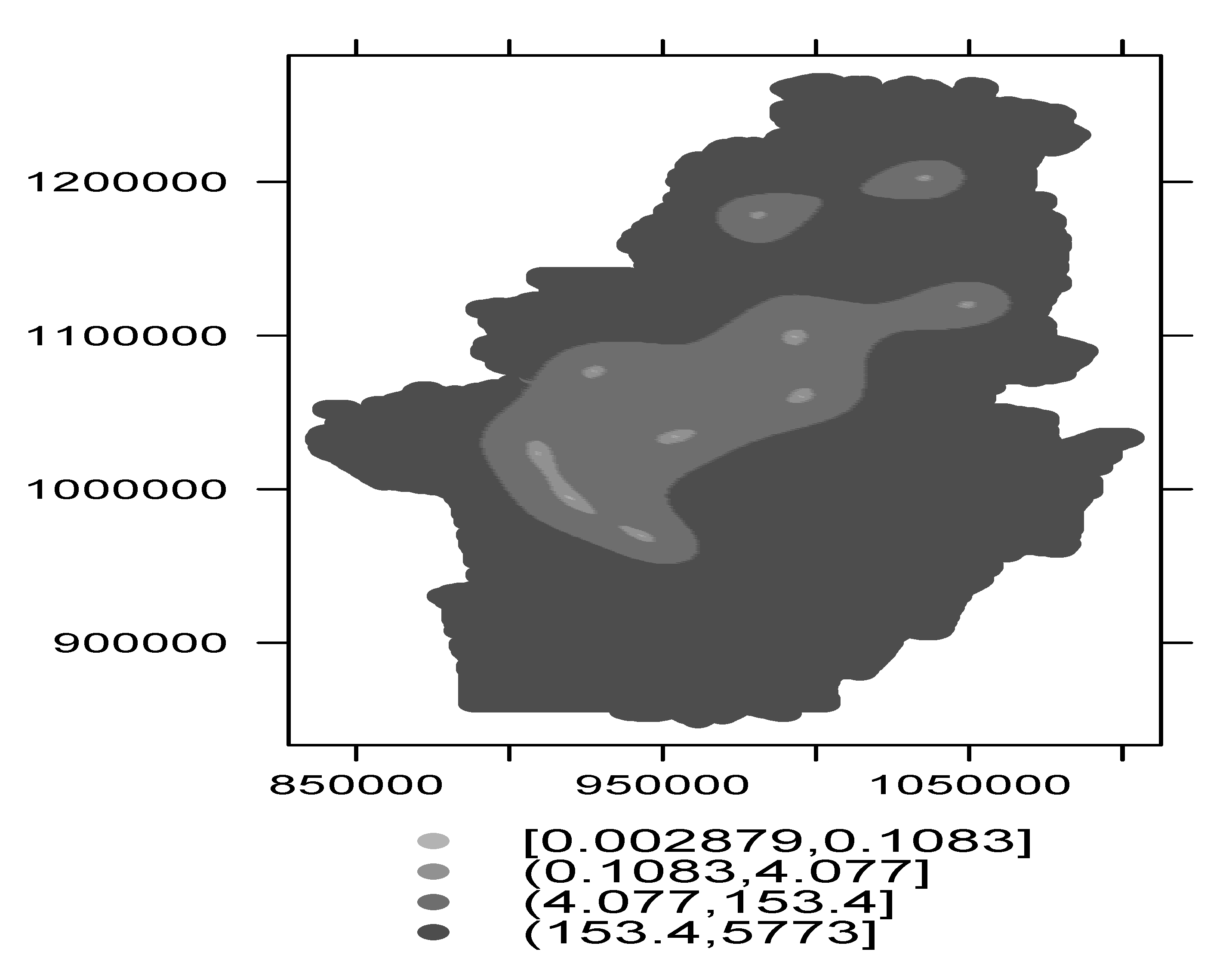
Second, the estimated CLM was used to derive the matrices Γ k k , for k = 1 , , m , defined in (A1) of the Appendix A, which contain the spatial dependence. Subsequently, the cokriging coefficients, λ i and α i j namely, for i = 1 , , n and j = 1 , , k , defined in (5), were obtained. A regular grid was established (with 10000 points) covering the study area. Thus, the cokriging prediction was performed at each of these points. A map with the predictions obtained is displayed in Figure 4. In addition, at each point, a prediction variance was estimated and whose results are shown graphically in Figure 5.

4. Concluding Remarks, Discussion, and Future Research

In this section, we provide conclusions of the technical aspects developed in this work and a discussion of the empirical study analyzed. In addition, some ideas on further work are mentioned.

4.1. Conclusions and Discussion

In this work, we have proposed a cokriging predictor using a functional secondary variable. We have used a co-regionalized linear model in order to estimate auto-correlations and cross-correlations.
From the application, the results were coherent with other studies that have described the behavior of PM10 in Bogotá city, one of the places with the worst air quality around the world, mainly due to the suspended material generated by mobile sources and the industrial sector [35]. Several aspects of PM10 behavior in the area under study can be mentioned. We started the analysis by assuming that the underlying stochastic process is stationary. Thus, we applied an ordinary cokriging predictor based on this assumption. However, some local variations were evident (above described with the bubble map of Figure 1). In general, it can be identified that, towards the south-west of the city, there are higher concentrations of PM10 and that towards the center and north-east the values tend to decrease as visualized in Figure 4. The highest concentrations were obtained in the industrial area of the city (darker grey) with values above 200.3 ( μ / g 3 ). From the central area of the city to the north (intermediate shades of gray), the values of PM10 fluctuate between 110 ( μ / g 3 ) and 200.3 ( μ / g 3 ). The lowest concentrations were found in the eastern zone (the area closest to the city’s hills). According to the map presented in Figure 5, there are areas with high prediction uncertainty (darker grey). These correspond to areas without monitoring stations; see Figure 1. As mentioned, there are areas near hills that have the lowest values of PM10, being it reasonable for us. However, the uncertainty of the prediction is high. Therefore, any interpretation from a practical point of view must be taken carefully. The same comment applies to other areas far away from the sampling stations.
In summary, this paper reported the following findings:
(i)
A cokriging predictor considering a functional secondary variable was proposed.
(ii)
After smoothing by using basis functions, an ordinary cokriging was defined by means of several secondary variables (as many as basis functions are used for smoothing the data).
(iii)
Cokriging was considered to be a better option than kriging, because including one or more secondary variables in the prediction process reduces uncertainty.
(iv)
It was showed how to use the proposed methodology when there are many measurements of a secondary variable over time.
(v)
An illustration with a real data set was considered to predict PM10 values in Bogotá city by using a cokriging predictor with wind speed as functional secondary variable.
The results of this work can be taken as a contribution to the explanation of the spatial variation of pollution within the city. Thus, our study can be a knowledge addition to the tool-kit of diverse practitioners, including environmental engineers, applied statisticians, and data scientists.

4.2. Further Work

Some themes for future research, which arose from the present investigation, are the following:
(i)
A cokriging predictor with functional variables can be studied upon non-stationarity [21].
(ii)
Extensions to the multivariate case is also of practical relevance [41].
(iii)
Incorporation of temporal and quantile regression structures in the modeling, as well as errors-in-variables, and PLS regression, are also of interest [42,43,44,45]
(iv)
The derivation of diagnostic techniques to detect potential influential cases are needed, which are an important tool to be used in all statistical modeling [44,46,47].
(v)
The applications of the new methodology proposed in this investigation can be of interest in diverse areas, where the functional data analysis is considered [29].
(vi)
It is of interest to study asymptotic behavior and performance of maximum likelihood estimators in spatial model [41,48].
(vii)
Autoregressive model-based fuzzy clustering can be used for detecting information redundancy in air pollution monitoring networks [49].
(viii)
Time series clustering by a robust autoregressive metric can be applied to the study of air pollution [50] and also other robust estimation methods when outliers are present into the data set [51].
Therefore, the proposed methodology in this investigation promotes new challenges and offers an open door to explore other theoretical and numerical issues. Research on these and other issues are in progress and their findings will be reported in future articles.

Author Contributions

Data curation, L.H. and R.G.; formal analysis, L.H., R.G. and V.L.; investigation, L.H., R.G. and V.L.; methodology, L.H., R.G. and V.L.; writing—original draft, R.G. and V.L.; writing—review and editing, V.L. All authors have read and agreed to the published version of the manuscript.

Funding

This research was supported partially by project grant “Fondecyt 1200525” (V. Leiva) from the National Agency for Research and Development (ANID) of the Chilean government.

Acknowledgments

The authors would also like to thank the Editor and Reviewers for their constructive comments which led to improve the presentation of the manuscript.

Conflicts of Interest

The authors declare no conflict of interest.

Appendix A

In this appendix, we provide some mathematical details of the cokriging system of equations, and of the coefficients of basis functions.

Appendix A.1. Cokriging System of Equations

The matrix representation of the cokriging system of equations to minimize the mean squared prediction error, subject to the unbiasedness constraints, by using the method of Lagrange multipliers, is given by
Γ 11 Γ 1 k Γ 1 m 1 0 0 Γ k 1 Γ k k Γ k m 0 1 0 Γ m 1 Γ m k Γ m m 0 0 1 1 0 0 0 0 0 0 1 0 0 0 0 0 0 1 0 0 0 λ α k α m δ 1 δ k δ m = γ 1 k γ k k γ m k 0 1 0 .

Appendix A.2. Coefficients of Basis Functions

The coefficients of basis functions can be obtained from
a i * = W a i = T ϕ 1 ( t ) ϕ 1 ( t ) d t T ϕ 1 ( t ) ϕ j ( t ) d t T ϕ 1 ( t ) ϕ k ( t ) d t T ϕ j ( t ) ϕ 1 ( t ) d t T ϕ j ( t ) ϕ j ( t ) d t T ϕ j ( t ) ϕ k ( t ) d t T ϕ k ( t ) ϕ 1 ( t ) d t T ϕ k ( t ) ϕ j ( t ) d t T ϕ k ( t ) ϕ k ( t ) d t a i 1 a i j a i k = l = 1 k a i l T ϕ 1 ( t ) ϕ l ( t ) d t l = 1 k a i l T ϕ j ( t ) ϕ l ( t ) d t l = 1 k a i l T ϕ k ( t ) ϕ l ( t ) d t = a i 1 * a i j * a i k * .

References

  1. Diggle, P.; Ribeiro, P. Model-Based Geoestatistics; Springer: New York, NY, USA, 2007. [Google Scholar]
  2. Cressie, N. Statistics for Spatial Data; Wiley: New York, NY, USA, 1993. [Google Scholar]
  3. Ver Hoef, J.; Barry, R. Constructing and fitting models for cokriging and multivariable spatial prediction. J. Stat. Plan. Inference 1998, 69, 275–294. [Google Scholar] [CrossRef]
  4. Chiles, J.; Delfiner, P. Geostatistics: Modeling Spatial Uncertainty; Wiley: New York, NY, USA, 1999. [Google Scholar]
  5. Marchant, C.; Leiva, V.; Cavieres, M.F.; Sanhueza, A. Air contaminant statistical distributions with application to PM10 in Santiago, Chile. Rev. Environ. Contam. Toxicol. 2013, 223, 1–31. [Google Scholar]
  6. Cappelli, C.; D’Urso, P.; De Giovanni, L.; Massari, R. Regime change analysis of interval-valued time series with an application to PM10. Chemom. Intell. Lab. Syst. 2015, 146, 337–346. [Google Scholar] [CrossRef]
  7. Leiva, V.; Marchant, C.; Ruggeri, F.; Saulo, H. Monitoring urban environmental pollution by bivariate control charts: New methodology and case study in Santiago, Chile. Environmetrics 2015, 30, e2551. [Google Scholar]
  8. D’Urso, P.; Cappelli, C.; De Giovanni, L.; Massari, R. Autoregressive metric-based trimmed fuzzy clustering with an application to PM10 time series. Chemom. Intell. Lab. Syst. 2017, 161, 15–26. [Google Scholar] [CrossRef]
  9. Marchant, C.; Leiva, V.; Christakos, G.; Cavieres, M.F. A criterion for environmental assessment using Birnbaum-Saunders attribute control charts. Environmetrics 2019, 26, 463–476. [Google Scholar]
  10. Cavieres, M.F.; Leiva, V.; Marchant, C.; Rojas, F. A methodology for data-driven decision making in the monitoring of particulate matter environmental contamination in Santiago of Chile. Rev. Environ. Contam. Toxicol. 2020. [Google Scholar] [CrossRef]
  11. Leiva, V.; Saulo, H.; Souza, R.; Aykroyd, R.G.; Vila, R. A new BISARMA time series model for forecasting mortality using weather and particulate matter data. J. Forecast. 2020. [Google Scholar] [CrossRef]
  12. Le, N.; Zidek, J. Statistical Analysis of Environmental Space-Time Processes; Springer: New York, NY, USA, 2006. [Google Scholar]
  13. Garcia-Papani, F.; Leiva, V.; Ruggeri, F.; Uribe-Opazo, M.A. Kriging with external drift in a Birnbaum-Saunders geostatistical model. Stoch. Environ. Res. Risk Assess. 2018, 32, 1517–1530. [Google Scholar] [CrossRef]
  14. Wackernagel, H. Cokriging versus kriging in regionalized multivariate data analysis. Geoderma 1994, 62, 83–92. [Google Scholar] [CrossRef]
  15. Helterbrand, J.; Cressie, N. Universal cokriging under intrinsic coregionalization. Math. Geol. 1994, 26, 205–226. [Google Scholar] [CrossRef]
  16. Rivoirard, J. Which models for collocated cokriging? Math. Geol. 2001, 33, 117–131. [Google Scholar] [CrossRef]
  17. Pardo-Igúzquiza, E.; Dowd, P. Multiple indicator cokriging with application to optimal sampling for environmental monitoring. Comput. Geosci. 2005, 31, 1–13. [Google Scholar] [CrossRef]
  18. Isaaks, E.; Srivastava, M. Applied Geostatistics; Oxford University Press: New York, NY, USA, 1989. [Google Scholar]
  19. Delicado, P.; Giraldo, R.; Comas, C.; Mateu, J. Geostatistics for spatial functional data: Some recent contributions. Environmetrics 2010, 21, 224–239. [Google Scholar] [CrossRef]
  20. Giraldo, R. Geostatistics for Functional Data. Ph.D. Thesis, Universitat Politècnica de Catalunya, Barcelona, Spain, 2009. [Google Scholar]
  21. Martinez, S.; Giraldo, R.; Leiva, V. Birnbaum-Saunders functional regression models for spatial data. Stoch. Environ. Res. Risk Assess. 2019, 33, 1765–1780. [Google Scholar] [CrossRef]
  22. Goulard, M.; Voltz, M. Geostatistical interpolation of curves: A case study in soil science. In Geostatistics Tróia’92; Soares, A., Ed.; Kluwer Academc Press: Dordrecht, The Netherlands, 1993; Volume 2, pp. 805–816. [Google Scholar]
  23. Nerini, D.; Monestiez, P.; Manté, C. Cokriging for spatial functional data. J. Multivar. Anal. 2010, 101, 409–418. [Google Scholar] [CrossRef]
  24. Giraldo, R.; Delicado, P.; Mateu, J. Ordinary kriging for function-valued spatial data. Environ. Ecol. Stat. 2011, 18, 411–426. [Google Scholar] [CrossRef] [Green Version]
  25. Menafoglio, A.; Petris, G. Kriging for Hilbert-space valued random fields. The operational point of view. J. Multivar. Anal. 2016, 146, 84–94. [Google Scholar] [CrossRef]
  26. Caballero, W.; Giraldo, R.; Mateu, J. A universal kriging approach for spatial functional data. Stoch. Environ. Res. Risk Assess. 2013, 27, 1553–1563. [Google Scholar] [CrossRef]
  27. Ignaccolo, R.; Mateu, J.; Giraldo, R. Kriging with external drift for functional data for air quality monitoring. Stoch. Environ. Res. Risk Assess. 2014, 28, 1171–1186. [Google Scholar] [CrossRef] [Green Version]
  28. Reyes, A.; Giraldo, R.; Mateu, J. Residual kriging for functional prediction of salinity curves. Commun. Stat. Theory Methods 2005, 44, 798–809. [Google Scholar] [CrossRef] [Green Version]
  29. Ramsay, J.; Silverman, B. Functional Data Analysis; Springer: New York, NY, USA, 2005. [Google Scholar]
  30. Hooyberghsa, J.; Mensinka, C.; Dumontb, G.; Fierensb, F.; Brasseurc, O. A neural network forecast for daily average PM10 concentrations in Belgium. Atmos. Environ. 2005, 39, 3279–3289. [Google Scholar] [CrossRef]
  31. Pérez, P.; Reyes, J. Prediction of maximum of 24-h average of PM10 concentrations 30 h in advance in Santiago, Chile. Atmos. Environ. 2002, 36, 4555–4561. [Google Scholar] [CrossRef]
  32. Giri, D.; Krishna-Murthy, V.; Adhiraky, P. The influence of meteorological conditions on PM10 concentrations in Kathmandu valley. Int. J. Environ. Res. 2008, 2, 49–60. [Google Scholar]
  33. Emery, X. Iterative algorithms for fitting a linear model of coregionalization. Comput. Geosci. 2010, 36, 1150–1160. [Google Scholar] [CrossRef]
  34. Giraldo, R. Propuesta de un indicador como variable auxiliar en el análisis cokriging. Rev. Colomb. Estadística 2001, 24, 1–12. [Google Scholar]
  35. Rodríguez-Camargo, L.; Sierra-Parada, R.; Blanco-Becerra, L. Análisis espacial de las concentraciones de PM2.5 en Bogotá según los valores de las guías de la calidad del aire de la Organización Mundial de la Salud para enfermedades cardiopulmonares, 2014–2015. Biomédica 2020, 40, 137–152. [Google Scholar] [CrossRef] [Green Version]
  36. Myers, D. Matrix formulation of cokriging. Math. Geol. 1982, 14, 249–257. [Google Scholar] [CrossRef] [Green Version]
  37. Bogaert, P. Comparison of kriging techniques in a space-time context. Math. Geol. 1996, 28, 73–86. [Google Scholar] [CrossRef]
  38. R Core Team. R: A Language and Environment for Statistical Computing; R Foundation for Statistical Computing: Vienna, Austria, 2018. [Google Scholar]
  39. Pebesma, E. Multivariable geostatistics in S: The gstat package. Comput. Geosci. 2004, 30, 683–691. [Google Scholar] [CrossRef]
  40. R Code. Available online: https://sites.google.com/a/unal.edu.co/ramon-giraldo-webpage/r-code (accessed on 20 July 2020).
  41. Sánchez, L.; Leiva, V.; Galea, M.; Saulo, H. Birnbaum-Saunders quantile regression models with application to spatial data. Mathematics 2020, 8, 1000. [Google Scholar] [CrossRef]
  42. Huerta, M.; Leiva, V.; Rodriguez, M.; Villegas, D. On a partial least squares regression model for asymmetric data with a chemical application in mining. Chemom. Intell. Lab. Syst. 2019, 190, 55–68. [Google Scholar] [CrossRef]
  43. Saulo, H.; Leão, J.; Leiva, V.; Aykroyd, R.G. Birnbaum-Saunders autoregressive conditional duration models applied to high-frequency financial data. Stat. Pap. 2019, 60, 1605–1629. [Google Scholar] [CrossRef] [Green Version]
  44. Carrasco, J.M.F.; Figueroa-Zuniga, J.I.; Leiva, V.; Riquelme, M.; Aykroyd, R.G. An errors-in-variables model based on the Birnbaum-Saunders and its diagnostics with an application to earthquake data. Stoch. Environ. Res. Risk Assess. 2020, 34, 369–380. [Google Scholar] [CrossRef]
  45. Sánchez, L.; Leiva, V.; Galea, M.; Saulo, H. Birnbaum-Saunders quantile regression and its diagnostics with application to economic data. Appl. Stoch. Model. Bus. Ind. 2020. [Google Scholar] [CrossRef]
  46. Garcia-Papani, F.; Leiva, V.; Uribe-Opazo, M.A.; Aykroyd, R.G. Birnbaum-Saunders spatial regression models: Diagnostics and application to chemical data. Chemom. Intell. Lab. Syst. 2018, 177, 114–128. [Google Scholar] [CrossRef] [Green Version]
  47. Liu, Y.; Mao, G.; Leiva, V.; Liu, S.; Tapia, A. Diagnostic analytics for an autoregressive model under the skew-normal distribution. Mathematics 2020, 8, 693. [Google Scholar] [CrossRef]
  48. Genton, M.G.; Zhang, H. Identifiability problems in some non-Gaussian spatial random fields. Chilean J. Stat. 2012, 3, 171–179. [Google Scholar]
  49. D’Urso, P.; Di Lallo, D.; Maharaj, E.A. Autoregressive model-based fuzzy clustering and its application for detecting information redundancy in air pollution monitoring networks. Soft Comput. 2013, 17, 83–131. [Google Scholar] [CrossRef]
  50. D’Urso, P.; De Giovanni, L.; Massari, R. Time series clustering by a robust autoregressive metric with application to air pollution. Chemom. Intell. Lab. Syst. 2015, 141, 107–124. [Google Scholar] [CrossRef]
  51. Velasco, H.; Laniado, H.; Toro, M.; Leiva, V.; Lio, Y. Robust three-step regression based on comedian and its performance in cell-wise and case-wise outliers. Mathematics 2020, 8, 1259. [Google Scholar] [CrossRef]
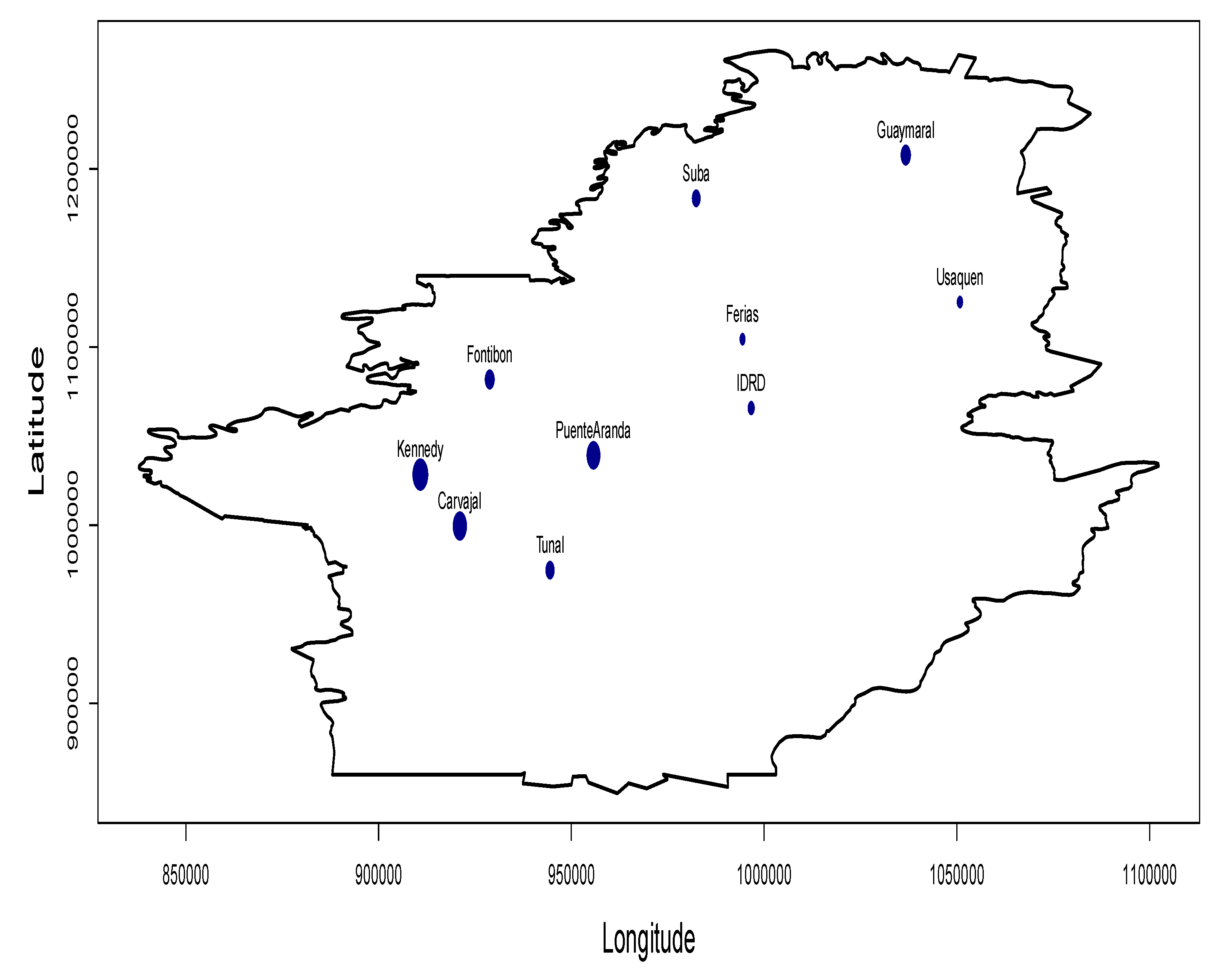
Figure 1. Spatial location of ten air quality monitoring stations in the Bogotá area. Circles are proportional to maximum PM10 values (maximum at each station was calculated based on data that were collected hourly between 26 January 2011 at 12:00 p.m. to 3 February 2011 at 2:00 p.m.).
Mathematics 08 01305 g001
Figure 2. WS values (in m/s) of ten air quality monitoring stations in the Bogotá area (data at each monitoring station were collected each two hours between 26 January 2011 at 10:00 a.m. to 3 February 2011 at 12:00 p.m.). In total, WS data were collected in 98 time periods (time period 1 corresponds to 10:00 a.m. of 26 January 2011 and time period 98 to 12:00 p.m. 3 February 2011).
Mathematics 08 01305 g002
Figure 3. WS curves obtained by smoothing the data set of each station using a Fourier basis (of dimension k = 7 ). Time period 1 corresponds to 10:00 a.m. 26 January 2011 and time period 98 to 12:00 p.m. 3 February 2011.
Mathematics 08 01305 g003
Figure 4. Map of PM10 predictions in the Bogotá area obtained with cokriging and a secondary variable corresponding to WS curves.
Mathematics 08 01305 g004
Figure 5. Map of PM10 prediction variances with the highest magnitudes (dark grey) corresponding to zones distant from the sampling sites.
Mathematics 08 01305 g005
Table 1. PM10 values and coefficients a i j , for  i = 1 , , n and j = 1 , , 7 , of Fourier basis functions fitted to SW data (collected each two hours between 26 January 2011 and 3 February 2011 at each of ten environmental monitoring stations in Bogotá, Colombia).
Station IDMonitoring StationPM10 a i 1 a i 2 a i 3 a i 4 a i 5 a i 6 a i 7
1Carvajal2424.352.311.871.40–0.40–0.10–0.67
2Fontibon17411.243.972.122.17–1.05–0.37–0.83
3Guaymaral1793.491.671.260.85–0.48–0.51–0.50
4Kennedy2659.763.521.721.54–0.55–0.05–0.60
5Las Ferias1166.902.171.370.91–0.69–0.26–0.56
6Simón Bolivar1305.772.131.520.88–0.27–0.48–0.24
7Puente Aranda2379.803.001.491.77–0.37–0.48–0.63
8Suba1576.410.761.630.51–0.13–0.83–0.23
9Tunal1624.641.941.271.07–0.33–0.01–0.35
10Usaquen1185.391.12-0.220.19–0.07–0.17–0.59