New Concepts in Intuitionistic Fuzzy Graph with Application in Water Supplier Systems

Abstract

In recent years, the concept of domination has been the backbone of research activities in graph theory. The application of graphic domination has become widespread in different areas to solve human-life issues, including social media theories, radio channels, commuter train transportation, earth measurement, internet transportation systems, and pharmacy. The purpose of this paper was to generalize the idea of bondage set (BS) and non-bondage set (NBS), bondage number $\alpha \left(G\right)$, and non-bondage number ${\alpha }_k\left(G\right)$, respectively, in the intuitionistic fuzzy graph (IFG). The BS is based on a strong arc (SA) in the fuzzy graph (FG). In this research, a new definition of SA in connection with the strength of connectivity in IFGs was applied. Additionally, the BS, $\alpha \left(G\right)$, NBS, and ${\alpha }_k\left(G\right)$ concepts were presented in IFGs. Three different examples were described to show the informative development procedure by applying the idea to IFGs. Considering the examples, some results were developed. Also, the applications were utilized in water supply systems. The present study was conducted to make daily life more useful and productive.

1. Introduction

Fuzzy graph models are advantageous mathematical tools for dealing with combinatorial problems of different domains including: algebra, environmental science, topology, optimization, social science, computer science, and operations research. Fuzzy graphical models are much better than graphical models due to natural existence of vagueness and ambiguity. Initially, we needed fuzzy set theory to cope with many complex phenomenons having incomplete information. A fuzzy set, as a superset of a crisp set, owes its origin to the work of Zadeh [1] in 1965 that has been introduced to deal with the notion of partial truth between absolute true and absolute false. Zadeh’s remarkable idea has found many applications in several fields, including chemical industry, telecommunication, decision making, networking, computer science, and discrete mathematics. Kauffman [2] introduced fuzzy graphs using Zadeh’s fuzzy relation [3]. Rosenfeld [4] gave an additional extended definition of a fuzzy graph (FG). He also continued to work on the ideas of graph theory in various fields like paths and connectivity. Since the concept of strong edges is useless in graphs, its importance in FGs cannot be neglected. In 1998, Somasundram [5] analyzed the domination in FGs by using effective edges. Gani et al. [6] also used the notion of strong arcs (SAs) to discuss the domination in FGs. Also, dominating sets consist of components in fault tolerance, wireless sensor network, and operational research, such as issues with the area of infrastructure. Bhutani [7] presented the concept of strong arcs. Gani [8] categorized vertices utilizing domination critical properties and studied the idea of increasing or reducing domination numbers by eliminating vertices. Gani et al. [9] conducted a study on the concept of bondage and non-bondage set ($NBS$) in FGs. They discovered bondage and ${\alpha }_k\left(G\right)$ of different classes of an FG and acquired upper bounds for both. Akram et al. [10,11,12,13,14,15,16] studied new concepts in different kinds of fuzzy graphs and fuzzy hypergraphs.

Membership function was not adequate enough to explain the complexity of object characteristics, and accordingly, there exists a non-membership function. Atanassov [17] developed the intuitionistic fuzzy set theory, which was an expansion of the initial set theory, by incorporating the non-membership and hesitancy features. This theory has been implemented in various fields such as computer programming, problems in decision-making, medical fields, marketing evaluation, and banking problems. In 2006, Karunambigai and Parvathi [18] introduced an intuitionistic fuzzy graph (IFG) as a specific case of the IFG by Atanassove. Fink et al. [19] developed the notion of $\alpha \left(G\right)$ in graphs. Kulli and Janakiram [20] first discovered the ${\alpha }_k\left(G\right)$ in graphs. Cockayne and Hedetniemi established [21] the domination number ($\eta \left(G\right)$) and the independent domination number of graphs but the theory of dominating sets in graphs was developed by Ore and Berge [22,23]. Later in 1994, Hartnell et al. [24] explored the bounds on the $\alpha \left(G\right)$. As each arc is strong, there is no idea of SA in graph theory, but finding an arc in IFGs is necessary. The research of weak and strong SAs was extensively laid out by Karunambigai et al. [25] depending on the connectivity strength of two vertices and extended to $\alpha$-$strong$ and $\delta$-$weak$ with relevant descriptions. Palanivel [26] examined several kinds of domination in IFGs. In 2012, Velammal and Karthikeyan [27] presented the notion of domination and complete domination in IFGs and defined the amount of domination and total domination number for various IFGs and obtained bounds for them. Similarly, Jayalakshmi et al. [28] expanded domination research and studied total strong-weak domination in IFGs.

The $\alpha \left(G\right)$ is a key factor of graphs that is focused on a well-known $\eta \left(G\right)$ and it is a key tool for determining the stability or the uncertainty of a domination in a graph or a network. Likewise, the concept of $\alpha \left(G\right)$ in fuzzy graphs has been developed to solve world life problems in many essential fields like school bus routing, computer communication networks, radio stations, land surveying, etc. The study on the $\alpha \left(G\right)$ was motivated by the increasing importance in the design and analysis of interconnection networks. Since then, the $\alpha \left(G\right)$ has attracted much attention from the researchers. If we take a fuzzy graph as a communication networks system, then, $\alpha \left(G\right)$ is a key factor, which is based upon $\eta \left(G\right)$. The domination is such an important and classic conception that it has become one of the most widely studied topics in fuzzy graph theory and also is frequently used to study properties of networks. The domination, with many variations and generalizations, is now well studied in fuzzy graph and networks theory.

The $BS$, $NBS$, $\alpha \left(G\right)$ and ${\alpha }_k\left(G\right)$ in an IFG are very rich both in theoretical developments and applications as compared to fuzzy graph. $\alpha \left(G\right)$ and ${\alpha }_k\left(G\right)$ of the intuitionistic fuzzy graph are more significant than the fuzzy graph. Also, $\alpha \left(G\right)$ and ${\alpha }_k\left(G\right)$ for the directed graphs are more significant than undirected graphs. In this paper, BS and NBS of an IFG were discussed and the $\alpha \left(G\right)$ and ${\alpha }_k\left(G\right)$ of IFG were defined. We found $\alpha \left(G\right)$ and ${\alpha }_k\left(G\right)$ in IFG. It was proven that the isolated edge of an IFG G constituted the $BS$ of G. Finally, we made an application in real-life problems.

2. Preliminaries

In this section, a few preliminary concepts and definitions are developed, which are used in the paper.

Definition 1

([23]). A graph is an ordered pair $G^{*}=(V,E)$, where V is the set of vertices or nodes of $G^{*}$ and E is the set of all arcs or lines or edges. Note that for an arc $\{x,y\}$, we usually use the somewhat shorter notation $xy$. Two nodes x and y in an undirected graph $G^{*}$ are called adjacent in $G^{*}$ if $xy$ is an arc of $G^{*}$. An arc in which the terminating points are the same is called a loop. A simple graph has no loop.

Definition 2

([9]). The $\alpha \left(G\right)$ of a graph G is the minimum cardinality of a set of arcs of G in which the removal from G resulted in a graph with the $\eta \left(G\right)$ larger than that of G. The ${\alpha }_k\left(G\right)$ of a graph is the maximum cardinality among all sets of arcs of H ⊆ E so that the $\eta \left(G\right)$ of $G-H$ is equal to the $\eta \left(G\right)$ of G. The domination number, $\eta \left(G\right)$, is the smallest number of vertices in any dominating set of G.

Definition 3

([1]). A fuzzy subset ϕ on a set X is a map $\varphi :X\to [0,1]$. A fuzzy (binary) relation on X is a fuzzy subset $\varphi :X\times X\to [0,1]$ on $X\times X$.

Definition 4

([4]). An FG is of the form $G=(\psi ;\varphi )$ which is a pair of mappings $\psi :V\to [0,1]$ and $\varphi :V\times V\to [0,1]$ and is defined as $\varphi (k_i,k_j)\le \psi \left(k_i\right)\wedge \psi \left(k_j\right)$, where for all vertices $k_i,k_j\in V$.

Definition 5

([29]). The edge $k_i$$k_j$ of G is called SA if $k_i$ and $k_j$ are adjacent.

Definition 6

([25]). An arc $(k_i,k_j)$ of an FG G is called SA if, ${\varphi }^{\infty }(k_i,k_j)=\varphi (k_i,k_j)$. An arc in G is called an isolated arc or edge if it is not adjacent to any arc in G. The connectedness strength between two vertices of $k_{i}and{k}_j$ is defined as the maximum strengths of all paths between $k_{i}and{k}_j$; and it is denoted by ${\varphi }^{\infty }(k_i,k_j)$ or $C{O}_{\left(G\right)}(k_i,k_j)$.

Definition 7

([17]). An intuitionistic fuzzy set A on the set X is characterized by a mapping ${\psi }_1:X\to [0,1]$, which is called as a membership function and ${\psi }_2:X\to [0,1]$, which is called as a non-membership function. An intuitionistic fuzzy set is denoted by $A=(X,{\psi }_1,{\psi }_2)$.

Definition 8

([25]). $\left(IFG\right)$ is of the form G = $[({\psi }_1,{\psi }_2),({\varphi }_1,{\varphi }_2)]$ is a set of functions ${\psi }_1:V\to [0,1]$, ${\psi }_2:V\to [0,1]$ and ${\varphi }_1:V\times V\to [0,1]$, ${\varphi }_2:V\times V\to [0,1]$ where

• $0\le {\psi }_1\left(k_i\right)+{\psi }_2\left(k_i\right)\le 1,$
• $0\le {\varphi }_1(k_i,k_j)+{\varphi }_2(k_i,k_j)\le 1,$
• ${\varphi }_1(k_i,k_j)\le {\psi }_1\left(k_i\right)\wedge {\psi }_1\left(k_j\right)$ and ${\varphi }_2(k_i,k_j)\le {\varphi }_2\left(k_i\right)\vee {\psi }_2\left(k_j\right)$.

3. $\mathbf{\alpha }\left(\mathit{G}\right)$ and ${\mathbf{\alpha }}_{\mathit{k}}\left(\mathit{G}\right)$ of IFG

In this section, we define BS, NBS, $\alpha \left(G\right)$, and ${\alpha }_k\left(G\right)$ in the IFG and also the $\alpha \left(G\right)$ for a complete IFG and some specific IFG are introduced.

Definition 9

($\mathbf{BS}$). Assume that G be an IFG. If there exists a set $H\subseteq S$ such that $\eta (G-H)>\eta \left(G\right)$, then H is called BS of G, where S is the set of all SAs in G.

Definition 10

($\mathbf{\alpha }\left(\mathit{G}\right)$). The $\alpha \left(G\right)$ of an IFG G is the minimum cardinality among all BSs of G.

Definition 11

($\mathbf{NBS}$). The set of SAs $H\subseteq S$ is called an NBS if $\eta (G-H)=\eta \left(G\right)$, where S is the set of all SAs in G.

Definition 12

(${\mathbf{\alpha }}_{\mathit{k}}\left(\mathit{G}\right)$). The ${\alpha }_k\left(G\right)$, is the maximum cardinality among all set of SAs in which $H\subseteq S$, such that $\eta (G-H)=\eta \left(G\right)$, where S is the set of all SAs of G.

Theorem 1.

If an IFG G has an isolated edge, then $\alpha \left(G\right)$ =1.

Proof. 

Let’s consider G an IFG with an isolated edge of p. Suppose that u and v are the terminating vertices of the isolated edge p. Accordingly, p is a SA and u or v belongs to the minimum dominating set of G, but not both. Thus, removing p results in u and v as isolated vertices. Therefore, both u and v are considered to belong to each dominating set of $G-p$. Subsequently, $\eta (G-p)>\eta \left(G\right)$ and $\left\{p\right\}$ is a BS of G. Hence ${\alpha }_{\left(G\right)}$ = 1. □

Theorem 2.

If G is an IFG and G* is a star, then $\alpha \left(G\right)$ =1.

Proof. 

If G is an IFG and G* is a star. In G, all arcs are SAs and the vertex in the center dominates all other vertices in G. Therefore, $\eta \left(G\right)$ = 1. By removing any one arc p from G, we have $\eta (G-p)=2>\eta \left(G\right)$. So each arc will form a BS and the bondage number of, ${\alpha }_{(}G)$ = 1. □

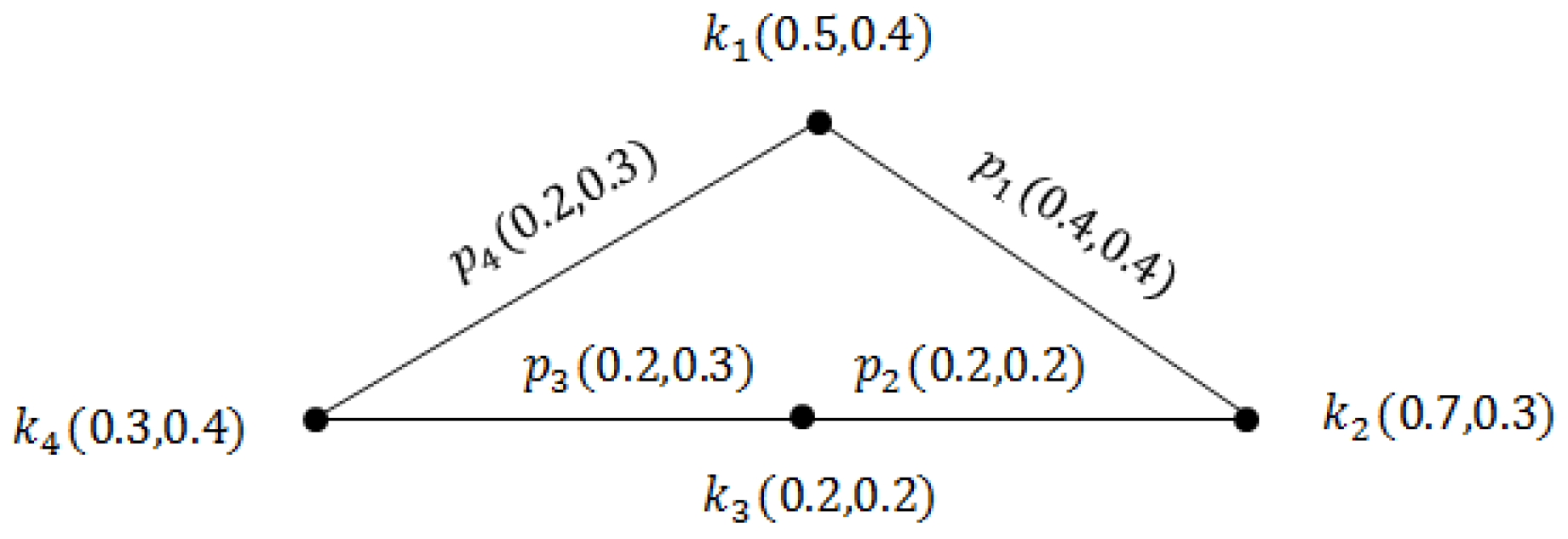
Example 1.

Consider IFG $G_1$ as shown in Figure 1. Calculating all the BSs and $\alpha \left(G\right)$ of the given graph.

Initially, we will calculate the SAs set in the mentioned graph. Now, we will calculate every arc connectedness (CO) strength in the graph.

For any two nodes of $k_i,k_j$∈ V, the ${\mu }_1$-strength of the connectedness and the ${\mu }_2$-strength of the connectedness are $C{O}_{\left(G\right)}(k_i,k_j)$ = $max\left\{S_{{\mu }_1}\right\}$, $C{O}_{\left(G\right)}(k_i,k_j)$ = $min\left\{S_{{\mu }_2}\right\}$, respectively including all paths of $k_{i}and{k}_j$.

We have to find $C{O}_{\left(G\right)}(k_1,k_2)=C{O}_{\left(G\right)}\left(p_1\right)$. There are two paths from $k_1$ to $k_2$.

The first path of $k_1$ to $k_2$ contains $p_1$ edge, but the second path of $k_1$ to $k_4$ to $k_3$ to $k_2$ contains $p_4$, $p_3$, and $p_2$ edges.

Now, we will find the strength of all paths.

The strength of the first path is $p_1$ because there is only a $p_1$ in it. Hence, the strength of path one is $p_1$ = (0.4, 0.4).

The strength of the second path is (min{0.2, 0.2, 0.2},max{0.3, 0.3, 0.2}) = (0.2, 0.3).

Now, we have the strength of all paths (0.4, 0.4) and (0.2, 0.3)

$$\begin{array}{c}C{O}_{\left(G\right)}(k_1,k_2)=C{O}_{\left(G\right)}\left(p_1\right)=(0.4\vee 0.2,0.4\wedge 0.3)=(0.4,0.3),\hfill \\ C{O}_{\left(G\right)}(k_2,k_3)=C{O}_{\left(G\right)}\left(p_2\right)=(0.2\vee 0.2,0.2\wedge 0.4)=(0.2,0.2),\hfill \\ C{O}_{\left(G\right)}(k_3,k_4)=C{O}_{\left(G\right)}\left(p_3\right)=(0.2\vee 0.2,0.3\wedge 0.4)=(0.2,0.3),\hfill \\ C{O}_{\left(G\right)}(k_1,k_4)=C{O}_{\left(G\right)}\left(p_4\right)=(0.2\vee 0.2,0.3\wedge 0.4)=(0.2,0.3).\hfill \end{array}$$

Since $p_1$ does not follow the condition ${\varphi }_{1ij}\ge CO{\left(G\right)}_{{\varphi }_1\left(G\right)}(k_i,k_j)$ and ${\varphi }_{2ij}\le CO{\left(G\right)}_{{\varphi }_2\left(G\right)}(k_i,k_j)$. Therefore the set of SAs will be

$$\begin{array}{c}\hfill S=\{p_2,p_3,p_4\}.\end{array}$$

The dominating set of G with the lowest cardinality is $F=\{k_3,k_4\}$. So the $\eta \left(G\right)$ is equal to,

$$\begin{array}{c}\eta \left(G\right)=\frac{1+0.3-0.4}{2}+\frac{1+0.2-0.2}{2}\hfill \\ \eta \left(G\right)=0.95.\hfill \end{array}$$

Since $BS$ of G is the subset of SAs in which the removal from IFG G results in a greater $\eta \left(G\right)$ of the resulting graph, we will calculate the BSs of G.

Suppose that $H=\left\{p_2\right\}$ is a subset of the set of SAs. We have to calculate SAs of $G-\left\{p_2\right\}$. First, any number of SAs is removed from the graph, and the required graph follows the conditions of ${\varphi }_{1ij}\ge CO{\left(G\right)}_{{\varphi }_1\left(G\right)}(k_i,k_j)$ and ${\varphi }_{2ij}\le CO{\left(G\right)}_{{\varphi }_2\left(G\right)}(k_i,k_j)$ as,

$$\begin{array}{c}C{O}_{\left(G\right)}(k_1,k_2)=C{O}_{\left(G\right)}\left(p_1\right)=(0.4,0.4),\hfill \\ C{O}_{\left(G\right)}(k_3,k_4)=C{O}_{\left(G\right)}\left(p_3\right)=(0.2,0.3),\hfill \\ C{O}_{\left(G\right)}(k_1,k_4)=C{O}_{\left(G\right)}\left(p_4\right)=(0.2,0.3).\hfill \end{array}$$

Therefore, the SA set will be,

$$\begin{array}{c}\hfill \{p_1,p_3,p_4\}.\end{array}$$

(1)

If the dominating set of $G-\left\{p_2\right\}$ with the lowest cardinality is $\{k_1,k_2\}$, then, its $\eta \left(G\right)$ will be,

$$\begin{array}{c}\eta \left(G-\left\{p_2\right\}\right)=\frac{1+0.5-0.4}{2}+\frac{1+0.3-0.4}{2}\hfill \\ \eta \left(G-\left\{p_2\right\}\right)=1.00>0.95.\hfill \end{array}$$

Hence $H=\left\{p_2\right\}$ is a $BS$.

Let’s consider $H=\left\{p_3\right\}$ as a subset of the SAs set. We will calculate the SAs of $G-\left\{p_3\right\}$. First any number of SAs is removed from the graph, the required graph follows the condition of ${\varphi }_{1ij}\ge CO{\left(G\right)}_{{\varphi }_1\left(G\right)}(k_i,k_j)$ and ${\varphi }_{2ij}\le CO{\left(G\right)}_{{\varphi }_2\left(G\right)}(k_i,k_j)$ as,

$$\begin{array}{c}C{O}_{\left(G\right)}(k_1,k_2)=C{O}_{\left(G\right)}\left(p_1\right)=(0.4,0.4),\hfill \\ C{O}_{\left(G\right)}(k_2,k_3)=C{O}_{\left(G\right)}\left(p_2\right)=(0.2,0.2),\hfill \\ C{O}_{\left(G\right)}(k_1,k_4)=C{O}_{\left(G\right)}\left(p_4\right)=(0.2,0.3).\hfill \end{array}$$

So the SA set will be,

$$\begin{array}{c}\hfill \{p_1,p_2,p_4\}.\end{array}$$

(2)

The $\{k_3,k_4\}$ is $G-\left\{p_3\right\}$ dominating set with the lowest cardinality and its $\eta \left(G\right)$ will be,

$$\begin{array}{c}\eta \left(G-\left\{p_3\right\}\right)=\frac{1+0.3-0.4}{2}+\frac{1+0.2-0.2}{2}\hfill \\ \eta \left(G-\left\{p_3\right\}\right)=0.95\ngtr 0.95.\hfill \end{array}$$

Therefore, $H=\left\{p_3\right\}$ is not a $BS$ bondage.

With a simple calculation similar to the above cases, we find that the BSs of giving IFG are:

$$\begin{array}{c}\hfill \left\{p_2\right\},\left\{p_4\right\},\{p_2,p_3\},\{p_2,p_4\},\{p_3,p_4\},\{p_2,p_3,p_4\}.\end{array}$$

The $BS$ with the lowest cardinality is $H=\left\{p_4\right\}$ and its cardinality is $\alpha \left(G\right)$ of G.

$$\begin{array}{c}\alpha \left(G\right)=\frac{1+0.2-0.3}{2}\hfill \\ \alpha \left(G\right)=0.45.\hfill \end{array}$$

Theorem 3.

The isolated edge of an IFG G constitutes the $BS$ of G.

Proof. 

Suppose that s is any isolated edge of the IFG G with the incident nodes of $k_1,k_2$. We know that s is isolated, and it follows the conditions of an SA as,

$$\begin{array}{c}\hfill {\varphi }_{1ij}=CO{\left(G\right)}_{{\varphi }_1\left(G\right)}(k_1,k_2)\\ \hfill {\varphi }_{2ij}\le CO{\left(G\right)}_{{\varphi }_2\left(G\right)}(k_1,k_2).\end{array}$$

(3)

So from both $k_1$ and $k_2$, one must be present in the dominating set of G, it is due to either $k_1$ dominates $k_2$ or $k_2$ dominates $k_1$. If we eliminate the s from G, both $k_1$ and $k_2$ will not be dependent and both of them will dominate themselves, giving a greater $\eta \left(G\right)$ of $G-s$ than G.

So s must be a $BS$ of G as its removal from G brings about the highest $\eta \left(G\right)$ than the G original $\eta \left(G\right)$, which is an axiom for $BS$ of G. □

Theorem 4.

For any IFG G, ${\alpha }_k\left(G\right)$ = $\mid E\mid$ - $\mid V\mid$ + $\eta \left(G\right)$.

Proof. 

Suppose that D is a minimum dominating set of G and therefore, $\mid D\mid$ = $\eta \left(G\right)$. For each vertex v$ϵV-D$, exactly select one SA which is incidental to nodes in D. Consider $S_1$ as the set of all these SAs. Then S-$S_1$ is a ${\alpha }_k$-set of G if G has no non-SAs. Assume that G has non-SAs, then every non-SA will form an SA by removing corresponding SAs in G. Therefore

$$\begin{array}{ccc}\hfill {\alpha }_k\left(G\right)& =& \mid S\mid -[\mid V\mid -\eta (G\left)\right]+\mid S\mid \hfill \\ & =& \mid S\mid +\mid E-S\mid +\eta \left(G\right)-\mid V\mid \hfill \\ & =& \mid E\mid -\mid V\mid +\eta \left(G\right).\hfill \end{array}$$

□

Theorem 5.

If IFG G does not have a BS, then ${\alpha }_k\left(G\right)$ =$\mid S\mid$.

Proof. 

Suppose that G is an IFG and it does not have a BS that is, there is not any set of $H\subseteq S$ so that $\eta (G-H)>\eta \left(G\right)$. Accordingly, removing all SAs from G does not increase the $\eta \left(G\right)$ of G. Now, by removing all SAs set, S, the $\eta \left(G\right)$ will be $\eta (G-S)=\eta \left(G\right)$. As a result, ${\alpha }_k\left(G\right)$ =$\mid S\mid$. □

Theorem 6.

For a complete IFG G,

$$\alpha \left(G\right)=\left\{\begin{array}{cc}{\displaystyle \frac{n}{2}},\hfill & ifniseven,\hfill \\ {\displaystyle \frac{(n+1)}{2}},\hfill & ifnisodd.\hfill \end{array}\right.$$

Proof. 

Suppose G is a complete IFG with n nodes namely $v_1,v_2,\dots ,v_n$. In G, every vertex dominates all other $n-1$ vertices. Therefore, $\left\{v_i\right\}$, $i=1,2,\dots ,n$ are all minimum dominating sets of G and $\eta \left(G\right)=1$. Now, eliminate the node $(v_1,v_2)$ then $v_1$ and $v_2$ dominate all $n-2$ vertices other than $v_2$ and $v_1$, respectively. Accordingly, we remove the edges $(v_3,v_4)$, $(v_5,v_6)$ and so on.

If n is even then delete the arcs $(v_1,v_2),(v_3,v_4),\dots ,(v_{n-3},v_{n-2})$ and $(v_{n-1},v_n)$. Thus, we get ${\displaystyle \frac{n}{2}}$ such edges and these form a BS of G. So $\alpha \left(G\right)={\displaystyle \frac{n}{2}}$. If n is odd then remove the edges $(v_1,v_2),(v_3,v_4),\dots ,(v_{n-2},v_{n-1})$ and $(v_n,v_1)$. Therefore, we obtain ${\displaystyle \frac{n+1}{2}}$ such edges and these form a BS of G. So, $\alpha \left(G\right)={\displaystyle \frac{n+1}{2}}$. □

Theorem 7.

If an IFG G has a BS, then $\alpha \left(G\right)\le {\alpha }_k\left(G\right)$+1.

Proof. 

Consider G as an IFG, which has a BS. A ${\alpha }_k\left(G\right)$-set is a maximum NBS, i.e., the elimination of all edges in a ${\alpha }_k\left(G\right)$-set results in $\eta \left(G\right)=\eta (G-{\alpha }_k)$. So, the deletion of any SA p does not belong to ${\alpha }_k$ with the arcs in the set ${\alpha }_k$ which results in $\eta (G-\{{\alpha }_k\cup p\})>\eta \left(G\right)$ implying that $\{{\alpha }_k\cup p\}$ is a BS.

Thus

$$\begin{array}{c}\hfill \alpha \left(G\right)\le \{{\alpha }_k\cup p\}={\alpha }_k\left(G\right)+1⟹\alpha \left(G\right)\le {\alpha }_k\left(G\right)+1.\end{array}$$

□

Theorem 8.

If G is an IFG and G* is a star then ${\alpha }_k\left(G\right)$ = 0.

Proof. 

Assume that G is an IFG and G* is a star. Then the $\eta \left(G\right)$ of G is 1, i.e., $\eta \left(G\right)$ = 1. It means that the vertex in the center of G dominates all remaining vertices in G. Therefore, elimination of any one edge of G will result in $\eta \left(G\right)$ = 2 since all edges of G are SAs in G. Accordingly, we do not have an NBS for G. Thus ${\alpha }_k\left(G\right)$ = 0. □

Theorem 9.

If G is a complete IFG with k nodes, then ${\alpha }_k\left(G\right)=(k-1)(k-2)/2$.

Proof. 

Let’s consider G as a complete IFG with k nodes. In G, all edges are strong. It means that the total number of SAs in G are $k(k-1)/2$. We know that $\eta \left(G\right)$ = 1. Each vertex will dominate all other vertices. Therefore, we need a minimum of $k-1$ arcs to keep $\eta \left(G\right)$ = 1. As a consequence, we can almost remove $\mid S\mid -(k-1)$ edges.

Therefore,

$$\begin{array}{c}{\alpha }_k\left(G\right)=\mid S\mid -(k-1)=k(k-1)/2-(k-1)=(k-1)(k/2-1)=(k-1)((k-2)/2),\hfill \\ {\alpha }_k\left(G\right)=(k-1)(k-2)/2.\hfill \end{array}$$

□

Theorem 10.

If G is an IFG and $G^{*}$ is a cycle with n nodes, then

$$\alpha \left(G\right)=\left\{\begin{array}{cc}3,\hfill & ifn=3m+1,m=1,2,\dots \hfill \\ 2,\hfill & else.\hfill \end{array}\right.$$

Proof. 

Suppose that G is IFG and $G^{*}$ is a cycle with n vertices.

(i)

Assume there is more than one weakest arc of G then all the n edges of G are SAs.

If $n=3m+1$, then $\eta \left(G\right)=m+1$.

The $\eta \left(G\right)$ rise only if we remove minimum 3 SAs. So, $\alpha \left(G\right)=3$.

If $n\ne 3m+1$, then the $\eta \left(G\right)$ rises when we remove a minimum of two SAs adjacent to the same vertices. Hence, $\alpha \left(G\right)=2$.

(ii)

Suppose that e is just one weakest arc of G, then G has $n-1$ SAs and elimination of any one SA gives the weakest arc as a SA in $G-e_1$, $e_1(\ne e)\in S$. Clearly, $\alpha \left(G\right)=3$, if $n=3m+1$ and $\alpha \left(G\right)=2$, if $n\ne 3m+1$. The weakest arc is not a part of any BS of G.

□

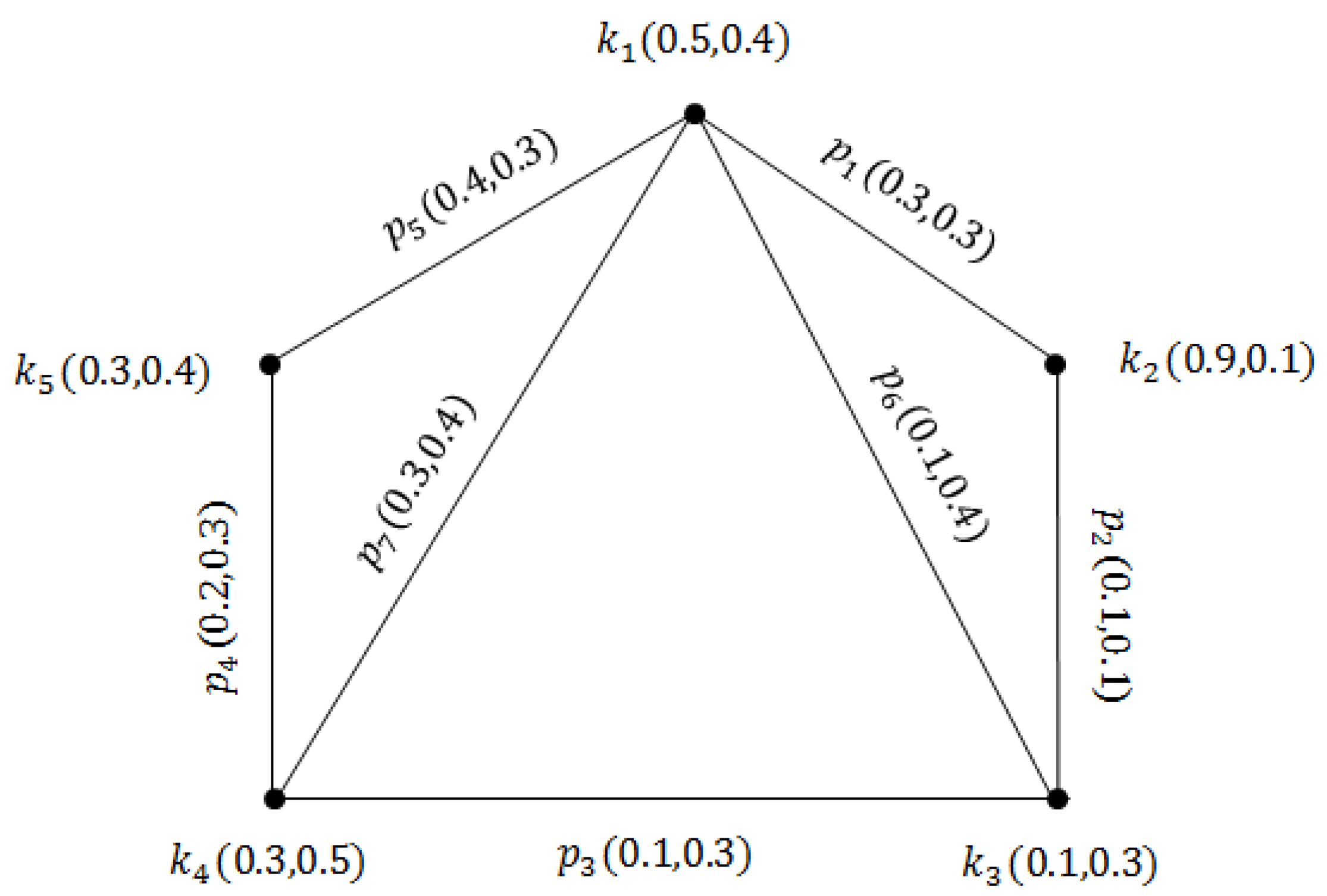
Example 2.

Consider IFG $G_2$ as shown in Figure 2. Applying the concept of $BS$ and $NBS$ on the following IFG.

First, we need to calculate the SAs of the given graph. Using the definition of SA in the IFG, we have:

$$\begin{array}{c}C{O}_{\left(G\right)}(k_1,k_2)=C{O}_{\left(G\right)}\left(p_1\right)=(0.3\vee 0.1\vee 0.1\vee 0.1,0.3\wedge 0.4\wedge 0.4\wedge 0.3)\hfill \\ =(0.3,0.3),\hfill \\ C{O}_{\left(G\right)}(k_2,k_3)=C{O}_{\left(G\right)}\left(p_2\right)=(0.1\vee 0.1\vee 0.1\vee 0.1,0.1\wedge 0.4\wedge 0.4\wedge 0.3)\hfill \\ =(0.1,0.1),\hfill \\ C{O}_{\left(G\right)}(k_3,k_4)=C{O}_{\left(G\right)}\left(p_3\right)=(0.1\vee 0.1\vee 0.1\vee 0.1,0.3\wedge 0.4\wedge 0.4\wedge 0.3)\hfill \\ =(0.1,0.3),\hfill \\ C{O}_{\left(G\right)}(k_4,k_5)=C{O}_{\left(G\right)}\left(p_4\right)=(0.2\vee 0.3\vee 0.1\vee 0.1,0.3\wedge 0.4\wedge 0.4\wedge 0.3)\hfill \\ =(0.3,0.3),\hfill \\ C{O}_{\left(G\right)}(k_1,k_5)=C{O}_{\left(G\right)}\left(p_5\right)=(0.4\vee 0.2\vee 0.1\vee 0.1,0.3\wedge 0.4\wedge 0.4\wedge 0.3)\hfill \\ =(0.4,0.3),\hfill \\ C{O}_{\left(G\right)}(k_1,k_3)=C{O}_{\left(G\right)}\left(p_6\right)=((0.1\vee 0.1\vee 0.1\vee 0.1,0.4\wedge 0.3\wedge 0.4\wedge 0.3)\hfill \\ =(0.1,0.3),\hfill \\ C{O}_{\left(G\right)}(k_1,k_4)=C{O}_{\left(G\right)}\left(p_7\right)=(0.3\vee 0.2\vee 0.1\vee 0.1,\mathrm{0.0.4}\wedge 0.3\wedge 0.4\wedge 0.3)\hfill \\ =(0.3,0.3).\hfill \end{array}$$

The SAs set of the given graph will be,

$$\begin{array}{c}\hfill \{p_1,p_2,p_3,p_5\}.\end{array}$$

The lowest dominating set with the lowest cardinality is,

$$\begin{array}{c}\hfill \{k_1,k_3\}.\end{array}$$

The $\eta \left(G\right)$ of the G can be calculated as,

$$\begin{array}{c}\eta \left(G\right)=\frac{1+0.5-0.4}{2}+\frac{1+0.1-0.3}{2}\hfill \\ \eta \left(G\right)=0.95.\hfill \end{array}$$

Since $BS$ of G is the subset of SAs in which the removal from IFG G will result in the greatest $\eta \left(G\right)$ of the resultant graph. We will now calculate BSs of G.

Let $H=\left\{p_1\right\}$ be a subset of the SAs set. To calculate the SAs of $G-\left\{p_1\right\}$, we have:

$$\begin{array}{c}C{O}_{\left(G\right)}(k_2,k_3)=C{O}_{\left(G\right)}\left(p_2\right)=(0.1,0.1),\hfill \\ C{O}_{\left(G\right)}(k_3,k_4)=C{O}_{\left(G\right)}\left(p_3\right)=(0.1\vee 0.1\vee 0.1,0.3\wedge 0.4\wedge 0.4)=(0.1,0.3),\hfill \\ C{O}_{\left(G\right)}(k_4,k_5)=C{O}_{\left(G\right)}\left(p_4\right)=(0.2\vee 0.3\vee 0.1,0.3\wedge 0.4\wedge 0.4)=(0.3,0.3),\hfill \\ C{O}_{\left(G\right)}(k_1,k_5)=C{O}_{\left(G\right)}\left(p_5\right)=(0.4\vee 0.2\vee 0.1,0.3\wedge 0.4\wedge 0.4)=(0.1,0.3),\hfill \\ C{O}_{\left(G\right)}(k_1,k_3)=C{O}_{\left(G\right)}\left(p_6\right)=((0.1\vee 0.1\vee 0.1,0.4\wedge 0.4\wedge 0.3)=(0.1,0.3),\hfill \\ C{O}_{\left(G\right)}(k_1,k_4)=C{O}_{\left(G\right)}\left(p_7\right)=(0.3\vee 0.2\vee 0.1,0.4\wedge 0.3\wedge 0.4)=(0.3,0.3).\hfill \end{array}$$

Using the SA definition, the SAs set will be,

$$\begin{array}{c}\hfill \{p_2,p_3,p_5\}.\end{array}$$

The dominating set of $G-\left\{p_1\right\}$ has the lowest cardinality of $\{k_1,k_3\}$, and its $\eta \left(G\right)$ will be,

$$\begin{array}{c}\eta \left(G-\left\{p_1\right\}\right)=\frac{1+0.5-0.4}{2}+\frac{1+0.1-0.3}{2}\hfill \\ \eta \left(G-\left\{p_1\right\}\right)=0.95\ngtr 0.95.\hfill \end{array}$$

As a result, $H=\left\{p_1\right\}$ is not a $BS$.

Suppose that $H=\left\{p_3\right\}$ to be a subset of the SAs set. To calculate the SAs of $G-\left\{p_3\right\}$, we have:

$$\begin{array}{c}C{O}_{\left(G\right)}(k_1,k_2)=C{O}_{\left(G\right)}\left(p_1\right)=(0.3\vee 0.1,0.3\wedge 0.4)=(0.3,0.3),\hfill \\ C{O}_{\left(G\right)}(k_2,k_3)=C{O}_{\left(G\right)}\left(p_2\right)=(0.1\vee 0.1,0.1\wedge 0.4)=(0.1,0.1),\hfill \\ C{O}_{\left(G\right)}(k_4,k_5)=C{O}_{\left(G\right)}\left(p_4\right)=(0.3\vee 0.1,0.3\wedge 0.4)=(0.3,0.3),\hfill \\ C{O}_{\left(G\right)}(k_1,k_5)=C{O}_{\left(G\right)}\left(p_5\right)=(0.3\vee 0.1,0.3\wedge 0.4)=(0.4,0.3),\hfill \\ C{O}_{\left(G\right)}(k_1,k_3)=C{O}_{\left(G\right)}\left(p_6\right)=(0.3\vee 0.1,0.3\wedge 0.4)=(0.1,0.3),\hfill \\ C{O}_{\left(G\right)}(k_1,k_4)=C{O}_{\left(G\right)}\left(p_7\right)=(0.3\vee 0.2,0.4\wedge 0.3)=(0.3,0.3).\hfill \end{array}$$

By using the SA definition, the SAs set will be,

$$\begin{array}{c}\hfill \{p_1,p_2,p_5\}.\end{array}$$

The dominating set of $G-\left\{p_3\right\}$ has the lowest cardinality of $\{k_1,k_3,k_4\}$, and its $\eta \left(G\right)$ will be,

$$\begin{array}{c}\eta \left(G-\left\{p_3\right\}\right)=\frac{1+0.5-0.4}{2}+\frac{1+0.1-0.3}{2}+\frac{1+0.3-0.5}{2}\hfill \\ \eta \left(G-\left\{p_3\right\}\right)=1.35>0.95.\hfill \end{array}$$

Accordingly, $H=\left\{p_3\right\}$ is a $BS$.

Suppose $H=\{p_1,p_2\}$ is a subset of the SAs. To calculate the SAs of $G-\{p_1,p_2\}$, we have:

$$\begin{array}{c}C{O}_{\left(G\right)}(k_3,k_4)=C{O}_{\left(G\right)}\left(p_3\right)=(0.1\vee 0.1\vee 0.1,0.3\wedge 0.4\wedge 0.3)=(0.1,0.3),\hfill \\ C{O}_{\left(G\right)}(k_4,k_5)=C{O}_{\left(G\right)}\left(p_4\right)=(0.2\vee 0.3\vee 0.1,0.3\wedge 0.4\wedge 0.4)=(0.1,0.3),\hfill \\ C{O}_{\left(G\right)}(k_1,k_5)=C{O}_{\left(G\right)}\left(p_5\right)=(0.4\vee 0.2\vee 0.1,0.3\wedge 0.4\wedge 0.4)=(0.2,0.3),\hfill \\ C{O}_{\left(G\right)}(k_1,k_3)=C{O}_{\left(G\right)}\left(p_6\right)=(0.1\vee 0.1\vee 0.1,0.4\wedge 0.4\wedge 0.3)=(0.1,0.3),\hfill \\ C{O}_{\left(G\right)}(k_1,k_4)=C{O}_{\left(G\right)}\left(p_7\right)=(0.3\vee 0.2\vee 0.1,0.4\wedge 0.3\wedge 0.4)=(0.3,0.3).\hfill \end{array}$$

Through using the SA definition, the set of SAs will be,

$$\begin{array}{c}\hfill \{p_2,p_4\}.\end{array}$$

The dominating set of $G-\{p_1,p_2\}$ has the lowest cardinality of $\{k_1,k_3\}$, and its $\eta \left(G\right)$ will be,

$$\begin{array}{c}\eta \left(G-\{p_1,p_2\}\right)=\frac{1+0.3-0.5}{2}+\frac{1+0.9-0.1}{2}\hfill \\ \eta \left(G-\{p_1,p_2\}\right)=1.3>0.95.\hfill \end{array}$$

Consequently, $H=\{p_1,p_2\}$ is a $BS$.

In the same way we can show that all the BSs of the given IFG are,

$$\begin{array}{c}\hfill \left\{p_3\right\},\{p_1,p_2\},\{p_1,p_3\},\{p_3,p_5\},\{p_1,p_2,p_3\},\{p_1,p_2,p_5\},\{p_1,p_2,p_3,p_5\}.\end{array}$$

These are the subsets of an SAs set in which the removal from G will result in a greater $\eta \left(G\right)$ of G. To calculate the $\alpha \left(G\right)$ of the given IFG, we must calculate the $BS$ with the lowest cardinality. The $BS$ has the lowest cardinality of $\left\{p_3\right\}$. Its cardinality is $\alpha \left(G\right)$ of G.

$$\begin{array}{c}\alpha \left(G\right)=\frac{1+0.1-0.3}{2}\hfill \\ \alpha \left(G\right)=0.4.\hfill \end{array}$$

Theorem 11.

If an NBS of G is an edge dominating set of G, then ${\alpha }_k\left(G\right)\ge {\displaystyle \frac{\eta \left(G\right)}{2}}$.

Proof. 

Let G be an IFG. Let D be an NBS of G and edge dominating set of G. Clearly, $\left|D\right|\ge {\eta }^{\prime }\left(G\right)$ and $\left|D\right|\le {\alpha }_k\left(G\right)$, ${\eta }^{\prime }\left(G\right)\le \left|D\right|\le {\alpha }_k\left(G\right)$, ${\eta }^{\prime }\left(G\right)\le {\alpha }_k\left(G\right)$.

We know that

$$\begin{array}{c}\eta \left(G\right)\le 2{\eta }^{\prime }\left(G\right)\hfill \\ \eta \left(G\right)\le 2{\eta }^{\prime }\left(G\right)\le 2{\alpha }_k\left(G\right).\hfill \end{array}$$

Hence, $\eta \left(G\right)\le 2{\alpha }_k\left(G\right)$, and so ${\displaystyle \frac{\eta \left(G\right)}{2}}\le {\alpha }_k\left(G\right)$. □

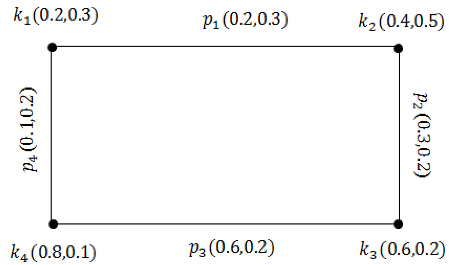
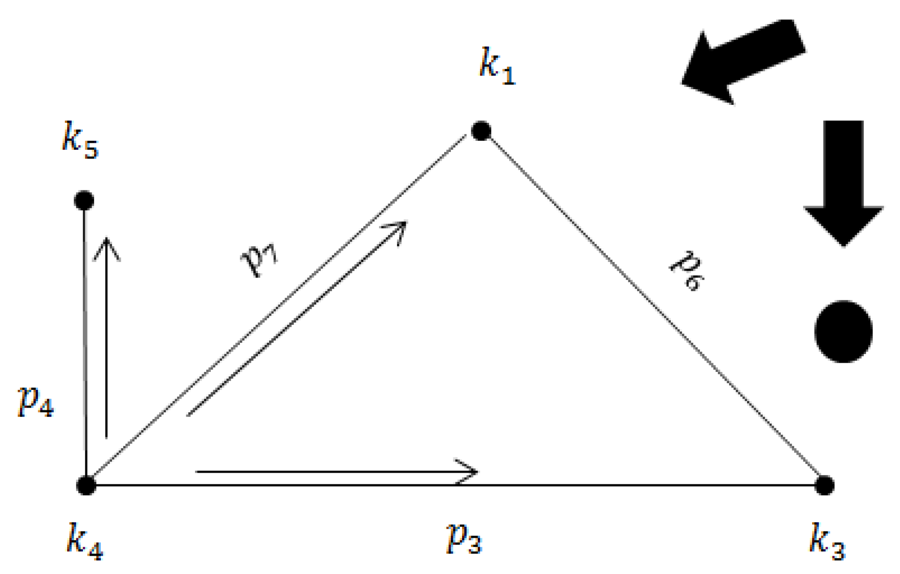
Example 3.

Consider IFG $G_3$, as shown in Figure 3, which is calculating all the NBSs and ${\alpha }_k\left(G\right)$ of a given graph.

First, we calculate the set of SAs in the given graph. Subsequently, we will calculate every arc connectedness strength in the graph.

$$\begin{array}{c}C{O}_{\left(G\right)}(k_1,k_2)=C{O}_{\left(G\right)}\left(p_1\right)=(0.1\vee 0.2,0.2\wedge 0.3)=(0.2,0.2),\hfill \\ C{O}_{\left(G\right)}(k_1,k_4)=C{O}_{\left(G\right)}\left(p_4\right)=(0.1\vee 0.2,0.2\wedge 0.3)=(0.2,0.2),\hfill \\ C{O}_{\left(G\right)}(k_2,k_3)=C{O}_{\left(G\right)}\left(p_2\right)=(0.3\vee 0.1,0.2\wedge 0.3)=(0.3,0.2),\hfill \\ C{O}_{\left(G\right)}(k_3,k_4)=C{O}_{\left(G\right)}\left(p_3\right)=(0.6\vee 0.1,0.2\wedge 0.3)=(0.6,0.2).\hfill \end{array}$$

Since $p_4$ and $p_1$ do not satisfy the condition of ${\varphi }_{1ij}\ge CO{\left(G\right)}_{{\varphi }_1\left(G\right)}(k_i,k_j)$ and ${\varphi }_{2ij}\le CO{\left(G\right)}_{{\varphi }_2\left(G\right)}(k_i,k_j)$, the set of SAs will be

$$\begin{array}{c}\hfill S=\{p_2,p_3\}.\end{array}$$

The dominating set of G has the lowest cardinality of $F=\{k_1,k_3\}$. As a result, the $\eta \left(G\right)$ will be,

$$\begin{array}{c}\eta \left(G\right)=\frac{1+0.2-0.3}{2}+\frac{1+0.6-0.2}{2}\hfill \\ \eta \left(G\right)=1.15.\hfill \end{array}$$

Since a $NBS$ of G is the subset of SAs in which the removal from IFG G will give an equal $\eta \left(G\right)$ of the resultant graph, we will now calculate non-BSs of G.

Let us consider $H=\left\{p_2\right\}$ to be a subset of the set of SAs. We will calculate SAs of $G-\left\{p_2\right\}$. After removing any number of SAs from the given graph, the remaining arcs of the graph satisfy the condition of ${\varphi }_{1ij}\ge CO{\left(G\right)}_{{\varphi }_1\left(G\right)}(k_i,k_j)$ and ${\varphi }_{2ij}\le CO{\left(G\right)}_{{\varphi }_2\left(G\right)}(k_i,k_j)$, because every pair of nodes is connected by a unique path that is the arc between them so their strength of connectedness is equal to the degrees of their arcs as,

$$\begin{array}{c}C{O}_{\left(G\right)}(k_1,k_2)=C{O}_{\left(G\right)}\left(p_1\right)=(0.2,0.3).\hfill \\ C{O}_{\left(G\right)}(k_3,k_4)=C{O}_{\left(G\right)}\left(p_3\right)=(0.6,0.2).\hfill \\ C{O}_{\left(G\right)}(k_1,k_4)=C{O}_{\left(G\right)}\left(p_4\right)=(0.1,0.2).\hfill \end{array}$$

So the SA set will be,

$$\begin{array}{c}\hfill \{p_1,p_3,p_4\}.\end{array}$$

(4)

The dominating set of $G-\left\{p_2\right\}$ with the lowest cardinality is $\{k_1,k_3\}$, and its $\eta \left(G\right)$ will be,

$$\begin{array}{c}\eta \left(G-\left\{p_2\right\}\right)=\frac{1+0.2-0.3}{2}+\frac{1+0.6-0.2}{2}\hfill \\ \eta \left(G-\left\{p_2\right\}\right)=1.15=1.15.\hfill \end{array}$$

Therefore, $H=\left\{p_2\right\}$ is an $NBS$.

Let’s assume $H=\left\{p_3\right\}$ as a subset of the set of SAs. The SAs of $G-\left\{p_3\right\}$, will be calculated as follows:

$$\begin{array}{c}C{O}_{\left(G\right)}(k_1,k_2)=C{O}_{\left(G\right)}\left(p_1\right)=(0.2,0.3),\hfill \\ C{O}_{\left(G\right)}(k_2,k_3)=C{O}_{\left(G\right)}\left(p_2\right)=(0.3,0.2),\hfill \\ C{O}_{\left(G\right)}(k_1,k_4)=C{O}_{\left(G\right)}\left(p_4\right)=(0.1,0.2).\hfill \end{array}$$

Accordingly, the SA set will be,

$$\begin{array}{c}\hfill \{p_1,p_2,p_4\}.\end{array}$$

(5)

The $\{k_1,k_2\}$ is the dominating set of $G-\left\{p_3\right\}$ with the lowest cardinality, and its $\eta \left(G\right)$ will be,

$$\begin{array}{c}\eta \left(G-\left\{p_3\right\}\right)=\frac{1+0.2-0.3}{2}+\frac{1+0.4-0.5}{2}\hfill \\ \eta \left(G-\left\{p_3\right\}\right)=0.9\ne 1.15.\hfill \end{array}$$

As a result, $H=\left\{p_3\right\}$ is not a $BS$.

Consider $H=\{p_2,p_3\}$ as a subset of the SAs set. We will calculate SAs of $G-\{p_2,p_3\}$, as:

$$\begin{array}{c}C{O}_{\left(G\right)}(k_1,k_2)=C{O}_{\left(G\right)}\left(p_1\right)=(0.2,0.3),\hfill \\ C{O}_{\left(G\right)}(k_1,k_4)=C{O}_{\left(G\right)}\left(p_4\right)=(0.1,0.2).\hfill \end{array}$$

Therefore, the SA set will be,

$$\begin{array}{c}\hfill \{p_1,p_4\}.\end{array}$$

(6)

The dominating set of $G-\{p_2,p_3\}$ has the lowest cardinality of $\{k_1,k_3\}$, and its $\eta \left(G\right)$ will be,

$$\begin{array}{c}\eta \left(G-\{p_2,p_3\}\right)=\frac{1+0.2-0.3}{2}+\frac{1+0.6-0.2}{2}\hfill \\ \eta \left(G-\{p_2,p_3\}\right)=1.15=1.15.\hfill \end{array}$$

Consequently, $H=\{p_2,p_3\}$ is an $NBS$.

All the NBSs of IFG are,

$$\begin{array}{c}\hfill \left\{p_2\right\},\{p_2,p_3\}.\end{array}$$

The $NBS$ has the highest cardinality of $H=\{p_2,p_3\}$. Therefore, the evaluation of its cardinality is as follows,

$$\begin{array}{c}{\alpha }_k\left(G\right)=\frac{1+0.3-0.2}{2}+\frac{1+0.6-0.2}{2}\hfill \\ {\alpha }_k\left(G\right)=1.25.\hfill \end{array}$$

So ${\alpha }_k\left(G\right)$ of the given IFG is obtained as ${\alpha }_k\left(G\right)=1.25$.

4. Application

We have found the $BS$ and number for some IFGs. Now we will try to find its applications in real life situations.

Water Supplier Systems

Water supply systems are tools for collecting, supplying, handling, transporting and delivering water for homes, industry, department, commercial and irrigation, as well as for government requirements, such as fire fighting and road flushing. The provision of portable water is perhaps the most important of all municipal services. People need water to drink, boil, do the laundry, prepare construction material, and other home needs. Water supply systems can serve public, financial and commercial demands. In all instances, the water must serve the demands both quantitatively and qualitatively. To discuss the application, we give Algorithm 1 as follows:

Consider a water supply system with the supply points and pipelines.

Considering it as an IFG, for labeling the parts of IFG, vertices constitute the supply points and the edges contain the systems pipelines. The membership degree of the supply points indicates the amount of water being delivered through these points, the degree of non-membership indicates the water is not delivered and the amount that has been dried up or lost from these points can be considered as a hesitant function.

A water flow rate or rupture rates varies with a period. The issue is inserted at the consumption level that has the lowest quantity of electric water to supply the water both to other supplies and to itself, which can only be supplied through SAs. Usually, higher water levels occur in the summer and smaller water price levels occur in the winter months, although this is not always the scenario in monsoon systems. SA in the setup process is a pipeline that can deliver the highest quantity of water from all the linked pipelines in a path. By identifying strong IFG arcs, pipelines with the largest flow can be described as the lowest number of supply points where the pumps can be fitted. If a water’s average flow is not sufficient for a limited water supply, a conservation reservoir may be constructed.

There is a problem where certain SAs or pipelines are blocked and cannot provide water. Adam blocks the stream of water, enabling the formation of an artificial lake. Conservation reservoirs hold much water for use during flooding and limited stream flow from moist climate phases. Inside the tank, a fluid supply system is constructed with multi-depth inlet pipes and pumps. Then what are the new supply points where the smallest number of pumps can be placed to supply the whole system with water?

Algorithm 1: Increasing Water Flow.

Pseudocode

Begin

Define IFG, supply points, pipelines

label the IFGvertices as supply points

label the IFG edges as pipelines

total water=membership degree+nono-membership degree

$f\left(hesitant\right)=$ non-membership degree supply

if current month falls (in summer monthe OR monsoon period)

water level=higher

else if

water level=lower

else if

Define strongest fiows

do i from 1 to$IFG.arcs.size$

if $IFG.arcs\left[i\right]$ is strng arc do

strongest flows.add ($IFG.arcs\left[i\right]$)

end if

end do

Fit pumps in all piplines in strongest flows

if $averageflows<sufficient$ do

construct conversation reservoir

end if

if $pipelines=blockedORSAs=blocked$

enable formation of artifical lake

end if

SAs to erase =BS Of IFG will inform

Insert pumps at supply points

$smalltanks=a\left(G\right)$

$V\left(tank\right)=\pi r^{2}l$

for each vertex v in $V\left[G\right]$ do

$d\left[v\right]:=\infty$

$parent\left[v\right]:=unknown$

end

$d\left[s\right]:=0$

$Q:=V$

while Q not empty do

$u:=TakeOffMin\left(Q\right)$

for each vertex $v-neighboru$ do

if $d\left[v\right]>d\left(u\right)+w(u,v)$ then

$d\left[v\right]:=d\left[u\right]+w(u,v)$

$previous\left[v\right]:=u$

else

Continue

end if

end

end

for each edge e in $E\left[G\right]$ do

$d\left[e\right]:=\infty$

$parent\left[e\right]:=unknown$

end

$d\left[s\right]:=0$

$Q:=E$

while Q not empty do

$f:=TakeOffMin\left(Q\right)$

for each edge $e-neighborf$ do

if $d\left[e\right]>d\left(f\right)+w(e,f)$ then

$d\left[e\right]:=d\left[f\right]+w(e,f)$

$previous\left[e\right]:=f$

else

Continue

end if

end

end

mark $p_1,p_2,p_3,p_5$ as strong pipelines

place pumps at $k_1,k_3$

mark $p_1,p_2,p_5$ blocked

frash domination range is $p_3,p_4,p_6,p_7$

End

The $BS$ of the IFG will inform us which SAs we can neglect, so we can get new supply points where the pumps can be inserted. To compensate for the limited capacity of a supply line, the volume of a tank must be designed. The $\alpha \left(G\right)$ will inform us by separating several powerful pipelines with which the system’s smallest effectiveness will be wasted. We can recognize the set of pipelines that has the smallest possible extraction effect system.

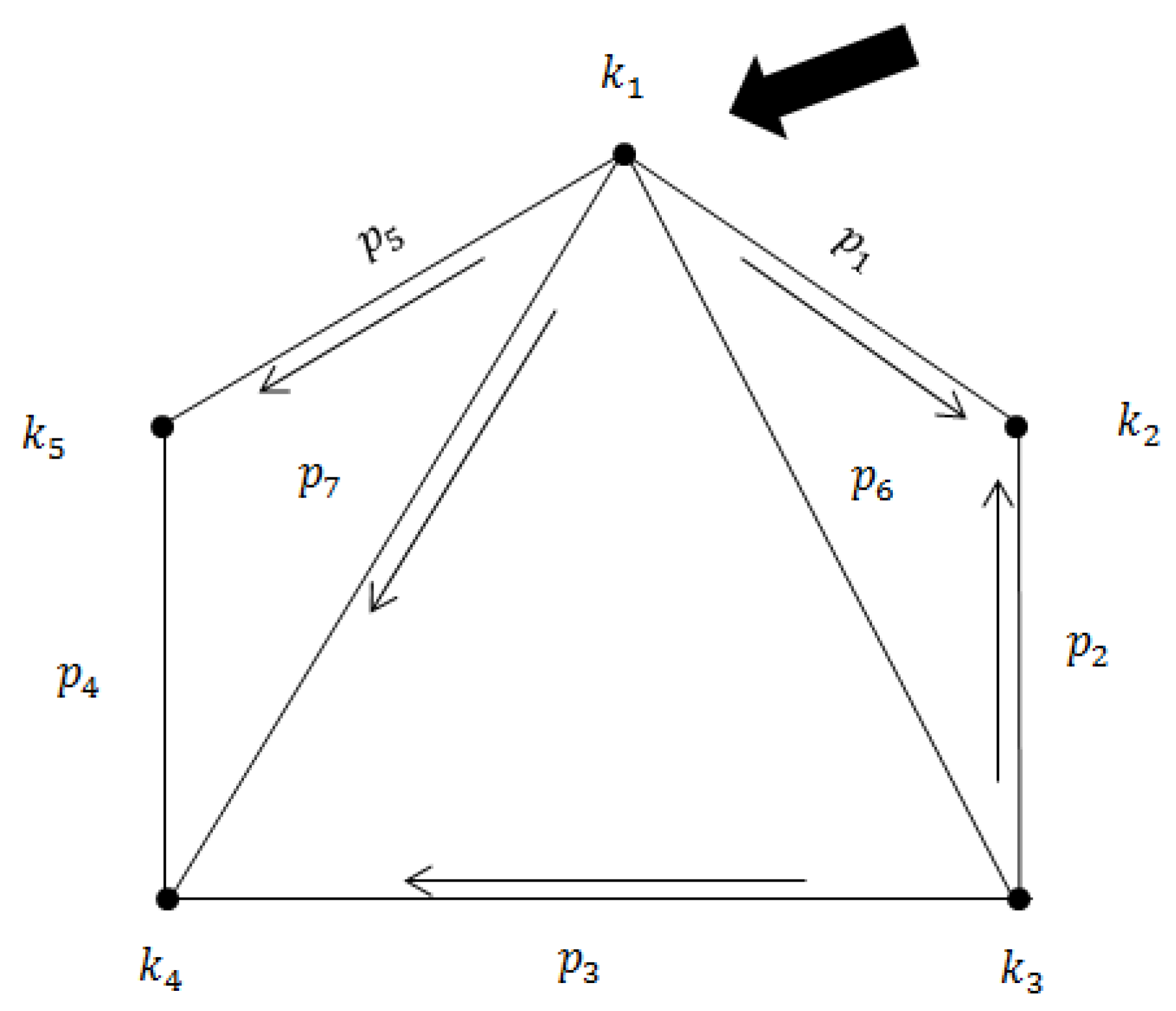
Considering example 3.2 as a water supplier as shown in Figure 4, the set of strong pipelines in the graph was $\{p_1,p_2,p_3,p_5\}$ and the lowest dominating set was $\{k_1,k_3\}$. So we will place the pumps at $k_1,k_3$ as,

Consider the position when some water system pipelines are blocked or destroyed and are unable to perform water flow. Let the pipelines be blocked at the edges of $\{p1,p2,p5\}$. The system has been removed, which means, it is added to the fresh scheme panels, while the fresh domination range is $\{p_3,p_4,p_6,p_7\}$, which is used to place the water pumps.

We can use the idea to discover the smallest amount of water supply points quickly as shown in Figure 5 ($G_5$) where it will be appropriate to locate the pump.

5. Conclusions

Intuitionistic fuzzy models are much better than FGs in precision, elasticity, and compatibility for the system. The IFG concept generally has a large variety of applications in different areas such as computer science, engineering and operational research. In this study, a description of results associated with extensions of certain ideas in IFGs was presented and their applications listed in this paper were more dynamic and realistic than FGs. Moreover, the $BS$ and $NBS$ concepts that already exist in IFGs were introduced and some results were established. A series of examples were given in IFGs that illustrated the concepts application method and its reliability. Using our approach to this idea, we inadvertently created a real-life application. This method adds uncertainty to the current techniques and opens the door to new research and application areas. The $\alpha \left(G\right)$ and ${\alpha }_k\left(G\right)$ of an IFG with examples were defined. Our future work is to apply this concept of BS, NBS, $\alpha \left(G\right)$ and ${\alpha }_k\left(G\right)$ on the vague graphs.