1. Introduction
Two-dimensional (2D) digital filters have been widely used in many areas of engineering, such as signal processing, computer vision, among others [
1,
2,
3]. Based on their impulse response, 2D filters are categorized into two main groups: Infinite impulse response (IIR) filters and finite impulse response (FIR) models. In general, IIR filters produce higher performance than their similar FIR models considering fewer parameters in their configuration [
4,
5]. However, since 2D-IIR filters easily produce unstable transfer functions, it is quite difficult to design them in comparison with their counterparts [
6].
The objective of filter design is to approximate the response of a determined filter to the desired behavior provided by the user requirements. The design methodologies for 2D-IIR filters can be grouped into two categories [
7,
8,
9]: transformation methods and optimization-based techniques. In a transformation method, the design of a 2D filter is constructed from a one-dimensional prototype that fulfills the required response. Under this scheme, filters are designed in a fast way, but adversely with low accuracy. On the other hand, in optimization-based techniques, the design of a 2D-IIR filter is interpreted as an optimization problem. Therefore, optimization algorithms are used to find the best suitable filter over a set of candidate solutions. Due to their synthesizing problems, the design of 2D-IIR filters is normally conducted through optimization tools instead of analytical methods [
10]. Under the optimization-based methodology, filters maintain a better accuracy than transformation methods. However, their design is highly dependent on the used optimization method. Normally, the generation of a filter through an optimization-based approach is computationally expensive and takes more time regarding transformation methods.
In optimization-based methods, the design process consists of finding the optimal parameters of a 2D-IIR filter that present the best possible resemblance with the desired response. To guide the optimization process, an objective function
J that evaluates the similarity between the candidate filter and the desired response must be defined. However, since 2D-IIR filters can easily produce unstable transfer functions, they tend to generate multimodal error surfaces, which are computationally difficult to optimize [
11]. This kind of objective function makes the operation of derivative-based techniques difficult since they can be easily trapped in a suboptimal solution [
12]. Under such conditions, approaches that use the gradient descent method as basis algorithms are scarcely considered for the design of 2D-IIR filters [
13].
On the other hand, EC techniques are optimization methods motivated in our scientific understanding of natural or social behavior, which at some abstraction level can be considered as search procedures [
14]. In the literature, EC approaches have shown better performance than those based on gradient methods in terms of robustness and accuracy [
12]. As a result, several design methods for 2D-IIR filters have been proposed considering different EC techniques such as the Particle Swarm Optimization (PSO) [
15], Genetic Algorithms (GA) [
16], and Artificial Bee Colony (ABC) [
17].
The capability of determining an optimal solution of an EC method is directly related to its ability to determine the balance between exploration and exploitation of the search space [
18] correctly. In the exploration stage the EC technique examines new solutions through the search space, while in the exploitation stage the local search of previously visited locations is carried out in order to improve its quality. If the exploration stage is mainly conducted, the efficiency of the optimization process is degraded, but the capability of determining new potential solutions increases [
19]. Otherwise, if the exploitation stage is privileged, the current solutions are highly refined. However, in this particular case, the technique achieves sub-optimal solutions as a result of a scarce exploration [
20]. Furthermore, each specific problem usually requires a different trade-off between both stages [
21]. Since the exploration–exploitation balance is an unsolved issue within EC community, each EC technique introduces an experimental solution through the combination of deterministic models and stochastic principles. Under such conditions, each EC technique holds distinctive characteristics that properly satisfy the requirements of particular problems [
22,
23,
24]. Therefore, a particular EC algorithm is not able to solve all problems adequately.
Recently, it has been also identified that each EC scheme presents a different tendency to analyze repeatedly certain areas of the search space or even outside the search space with the independence of the obtained objective function values. This effect is presented as a result of the operation of the specific operators of each EC method or in the early stages of the evolution process. Since this fact adversely affects the obtained results for each EC method, some strategies [
25] have been suggested to handle this problem. Among these techniques, the appropriate configuration of parameters represents one of the most common strategies reducing this effect and other undesired behaviors.
In order to determine the advantages and limitations of EC methods, their correct evaluation is an important task in the computational intelligence community. In general, EC algorithms are complex pieces of software with several operators and stochastic branches. Under such circumstances, appropriate statistical methods must be considered for obtaining significant conclusions. Although several comparisons among EC methods have been reported in the literature [
26,
27,
28], their conclusions are based on a set of synthetic functions, without considering the context of the problem or appropriate statistical treatment.
This paper reports a comparative study of various EC techniques when they are applied to the complex application of 2D-IIR filter design. In the comparison, special attention is paid to the most popular EC algorithms currently in use, such as PSO, ABC, DE, HS, GSA and FPA. In the experiments, the statistical analysis of Wilcoxon and Bonferroni has been conducted to validate the results obtained by these techniques.
The rest of this manuscript is organized as follows: In
Section 2, a brief description of each algorithm used in the comparison is presented. In
Section 3 the 2D-IIR filter design problem is formulated from the optimization point of view. The experimental results and the statistical analysis are presented in
Section 4. In
Section 5, a discussion is conducted. Finally, in
Section 6 the conclusions are reported.
2. Evolutionary Computation Techniques
Evolutionary computation (EC) techniques are powerful tools for solving complex optimization problems. Different from classical methods, EC algorithms are mainly appropriated to face multimodal objective functions.
Most of the EC techniques are inspired by nature or social phenomena, which a certain abstraction level can be considered as an optimization process. In general, EC techniques are formed of two principal components: determinist rules and stochastic operations. Combining both elements, each EC method proposes a particular solution to the exploration–exploitation balance. Under such conditions, each EC technique holds distinctive characteristics that appropriately fulfill the requirements of particular problems.
Several EC methods have been proposed in the literature. According to their applications [
14], the algorithms Particle Swarm Optimization (PSO) [
29], the Artificial Bee Colony (ABC) algorithm [
30], the Differential Evolution (DE) method [
31], the Harmony Search (HS) strategy [
32], the Gravitational Search Algorithm (GSA) [
33] and the Flower Pollination Algorithm (FPA) [
34] are considered the most popular currently in use. Therefore, they will be used in our comparison study. In this Section, a description of each algorithm used in the comparison is presented.
2.1. Particle Swarm Optimization (PSO)
The PSO is probably the most popular optimization technique; it was introduced by Kennedy in 1995 [
29], and is motivated by the action of bird flocking or fish schooling. The algorithm uses a group or swarm of particles as possible solutions
of
N particles, which are evolved from an initial point
to a maximum number of generations (
k = max_gen). Each particle
symbolizes a
d-dimensional vector
where each dimension is a decision variable of the treated problem. After initializing the particles randomly through the search space, each particle
is evaluated by the fitness function
, the best value of fitness during the evolution process is stored in a vector
with their respective positions
.
For practical proposes, the PSO implemented has been proposed by Lin in [
35], which compute a new position
of each particle
as follows:
where
is the inertia weight, and rules the current and the updated velocity,
and
are positive numbers that control the acceleration of each individual to the positions
g and
, respectively.
and
are random numbers in the interval [0, 1].
2.2. Artificial Bee Colony (ABC)
The ABC was introduced by Karaboga [
30]. It is based on the intelligent foraging behavior of honeybee swarms. In the ABC implementation, the algorithm generates a population
of
N possible food locations, which are evolved from the initial point
to the maximum number of generations (
k = max_gen). Each food position
symbolizes a
d-dimensional vector
where each dimension is a decision variable of the treated problem. The initial feasible food locations (solutions) are evaluated by an objective function to determinate which food location represents a satisfactory solution (nectar-amount) or not. Once the values from a cost function are computed, the candidate solution
evolves by different ABC operators (honeybee types), where each food location
generates a new food source
and is computed as follows:
where
is a food location randomly selected, which satisfies the condition
. A factor
is a random number in the interval [−1, 1]. When a new solution
is produced, a probability associated with the fitness value of a particular solution
is calculated. The quality of the solution determined by the fitness function can be assigned to the solution
using the following expression:
where
describes the cost function to be optimized. When the fitness values of the complete population are computed, a greedy selection between
and
is employed. If the quality of
is better than
then the solution
is changed by
; otherwise, the original solution remains.
If a candidate solution i (food source) cannot improve within a set trial value named as “limit”, the candidate solution is expected to be discarded and the related bee becomes a scout. A scout explores the search space without any information. To verify if a candidate solution reached the fixed “limit”, a counter is assigned to every food source i. The counter is incremented, resulting in a bee-operator failing to improve the food source’s quality.
2.3. Differential Evolution (DE)
The DE was developed by Storn and Price [
31], where the feasible solution is defined as a vector and is represented as follow:
where
is the
i-th vector at iteration
t. The standard DE procedure has three main stages:
(A) mutation, (B) crossover and
(C) selection which are described below:
(A) Mutation. This process is applied to a given vector
at the
t generation. Firstly, three different vectors are randomly selected from the entire population:
,
and
, then, a new vector (candidate solution) is generated as follow:
where
is a parameter related to the differential weight and is adjusted depending on the problem to be optimized.
(B) Crossover. This operator controlled by the crossover rate
. The
helps to modify only a few vectors of the population and it is applied on each dimension (or element) of a solution. The crossover begins by generating a random number
and then, the
j-th component
is handled as follow:
(C) Selection. The selection process is essentially the same as that used in Genetic Algorithms (GA) [
16]. The new solution is evaluated by the fitness function; if the new candidate solution is better than the current, then it is replaced. We can consider the following criteria:
2.4. Harmony Search (HS)
The HS was proposed by Geem [
32]; this algorithm is based on music. It was inspired by the observation that music aims are searching for the perfect state of harmony by improvisation. The analogy in optimization is the process of searching the optimal value of a problem. When a musician is improvising, he follows three rules to obtain a good melody: plays any well-known portion of music precisely from his memory, plays something similar to a famous piece and composes new music or plays random notes. In the HS operation those rules become;
(a) Harmony Memory (HM) consideration, (b) pitch adjustment and
(c) initialize a random solution.(a) Harmony Memory (HM) Consideration. This stage will guarantee that the best harmonies will be transferred to a new harmony memory. To apply the HM more efficiently, it is assigned a parameter that helps to select the elements of HM. Such a parameter is the Harmony Memory Consideration Rate (HMCR) and is defined as . If the value of the HMCR is low, only a few good harmonies are chosen and it can slowly converge. If such a value is notably high, most of the harmonies are employed in HM, and then additional harmonies are not used in the exploration stage.
(b) Pitch Adjustment. Each element achieved by memory consideration is additionally analyzed to decide whether it should be pitch-modified. For this action, the Pitch-Adjusting Rate (
PAR) is described to select the recurrence of the adjustment and the Bandwidth value (
BW) to regulate the local search of the chosen elements of the HM. Therefore, the pitch adjust determination is computed as:
Pitch modification is responsible for producing new likely harmonies by lightly adjusting original value positions. This action can be considered as the mutation rule in evolutionary techniques. Consequently, the decision variable is either modified by a random number in the range [0, BW] or remains with no changes.
(c) Initialize a random solution. This operation tries to increase the diversity of the solutions. As is mentioned in a), if a new solution is not taken from the harmony memory, it must be created randomly in the search space. It helps to explore new areas avoiding the local optimal. This process is described as follows:
where
HMS is the size of the HM,
is an element chosen from the HM, and
u and
l are the upper and lower bounds. Finally, rand is a random value uniformly distributed between 0 and 1.
2.5. Gravitational Search Algorithm (GSA)
The GSA is an evolutionary technique inspired by the Newtonian laws of gravity [
33]. The GSA has been used widely in different engineering fields due to its capabilities for determining competitive solutions [
36]. In GSA each mass (solution) represents a
d-dimensional vector
;
, at time
t, the mass
i acts to the mass
j in the variable
h with force defined as:
where
is the active gravitational mass associated with the solution
j,
represents the passive gravitational mass of the element
i,
is a gravitational constant at the time
t,
is a small constant, and
is the distance between the elements
i and
j. The
G(
t) function is adjusted through the evolution process for balancing the exploration and exploitation by the modification of attraction forces between solutions. The total force operating over the solution
i is represented as follows:
The acceleration at time
t of the candidate solution is estimated as below:
where
describes the inertial mass of the solution
i. The new location of each individual
i is calculated as:
The inertial and gravitational masses of each individual are estimated directly by its fitness function value. Consequently, the inertial and gravitational masses are updated by the following expressions:
where
describes the cost function that determines the quality of the solutions.
2.6. Flower Pollination Algorithm (FPA)
The FPA was introduced by Xin-She Yang in 2012 [
34]. FPA stimulates the flower pollination process of plants. In the biological approach, this process is key for the reproduction of a plant and is associated with the transfer of pollen. This transfer process is performed by pollinator agents (insects, birds, the wind, etc.). Pollination can be classified into two forms: abiotic and biotic. Most of the plants use biotic pollination, in which the use of external pollinator is necessary; this process is known as cross-pollination. On the other hand, abiotic pollination is known as self-pollination; it does not require the intervention of any external pollinator. Contrarily to the biological approach, the FPA for simplicity contemplates just one flower that provides one pollen gamete. In the FPA, a solution
corresponds to a flower or pollen gamete. In the implementation, the algorithm generates a population
of
m flowers, where each flower is represented by a
d-dimensional vector
. The dimension vector
d corresponds to the number of decision variables of the problem to treat.
(A) Lévy flights. One of the most powerful operators in flower pollination algorithm is the
Lévy Flights [
37], which generates a random walk. The walk length is defined by a heavy-tailed probability distribution. The random walk is generated as follows:
where
and
are vectors of dimensionality
d, and the value
. The elements of the vectors
u and
v are computed using normal distributions as below:
where
represents the Gamma distribution.
(B) Local pollination. The local pollination is described in Equation (19), where
and
are pollens from two different flowers of the same plant species.
where
is a scalar random value within [0, 1].
(C) Global pollination. The original position
is replaced with the new position
according to the following equation:
where
is a random scalar within [0, 1] while
is the best candidate solution seen so-far.
3. 2D-IIR Filter Design Process as an Optimization Problem
This section formulates the process of the 2D-IIR filter design as an optimization problem. In this paper, the zero-phase IIR filter design is considered. A zero-phase filter is a particular example of linear phase filters where the phase slope is zero. This fact suggests that the impulse response is always even (
) [
8]. The structure of a 2D-IIR filter is presented in Equation (21) [
15,
16,
38,
39,
40].
where
,
,
,
are the filter coefficients,
is an intensity constant while
K symbolizes the filter order. In case of
K = 2, the model of Equation (21) corresponds to a 2nd order filter whereas a higher value (
K > 3) specifies a high order filter. In Equation (21), it is usually configured
(by normalizing
to the value of
).
and
represent complex variables in the
z-transform domain. However, for convenience, the Fourier frequency domain is used, where
and
are defined as follows:
where
j is the imaginary constant and
are frequency variables. With the substitution of Equation (22) in Equation (21),
changes to
.
The objective of filter design is to approximate the response of a determined 2D-IIR filter structure to the desired behavior provided by the user requirements. Therefore, the design process consists of finding the optimal parameters that present the best possible resemblance with the desired response Both responses and are discretely computed at points.
To guide the search process, an objective function
J that evaluates the similarity between the candidate filter
and the desired response
must be defined. This similarity can be defined as the difference that exists between both responses, such as follows:
where
,
. For the sake of clarity, the Equation (23) can be rewritten as:
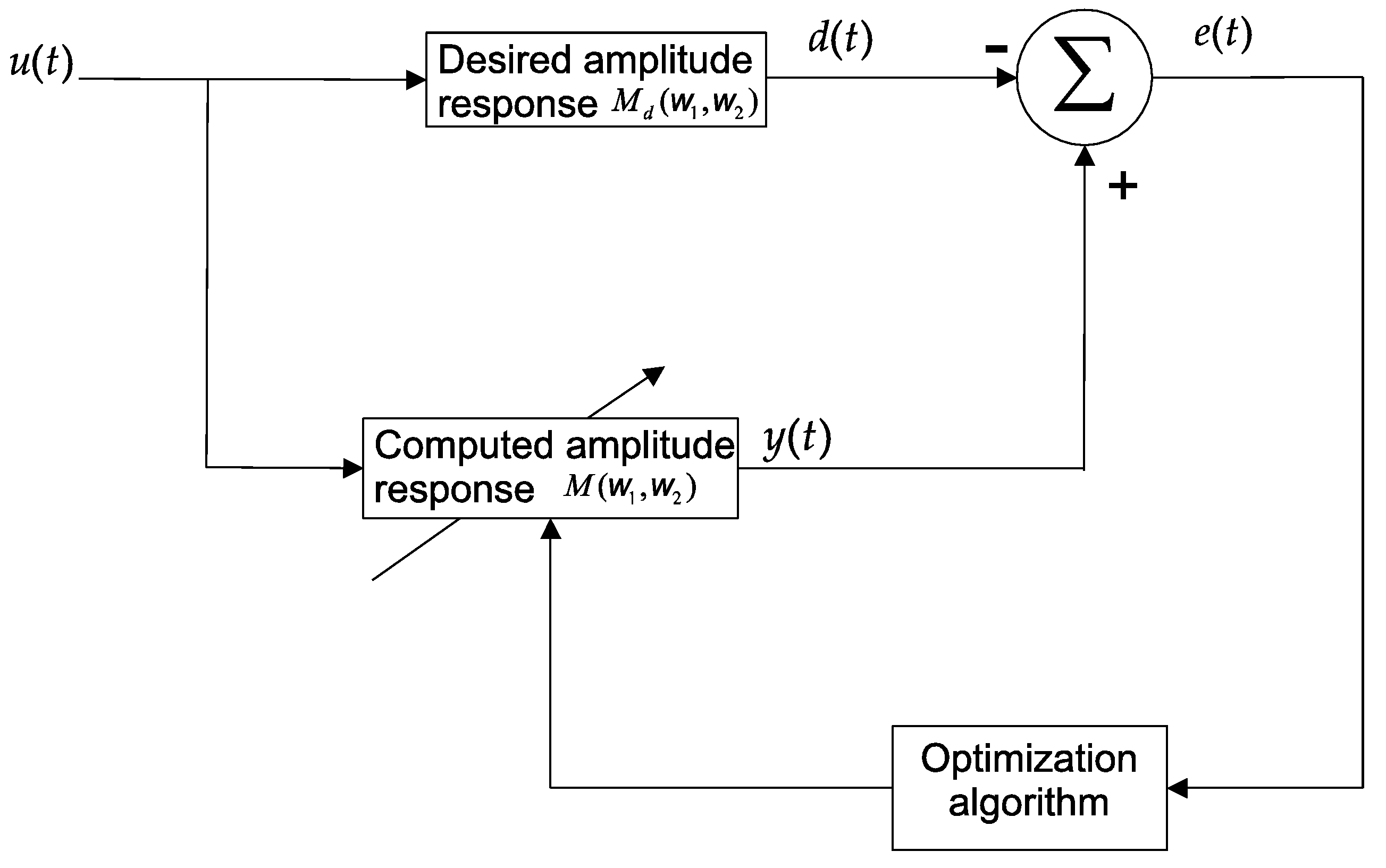
Figure 1 illustrates the filter design process. In the learning schema, the difference between the computed (
y(
t)) and desired (
d(
t)) filter response is used to guide the evolution process.
One main difficulty of 2D IIR filters is the tendency to produce unstable transfer functions. Therefore, in the evaluation of Equation (24), it is necessary to verify if the poles of the transfer function are located within the unitary circle of the
z-plane. To validate this state, several conditions must be fulfilled, which, for Equation (25) can be expressed as follows [
15,
16,
38]:
Under such circumstances, the filter design process can be translated into an optimization problem with constraints.
Comparison Setting
In order to conduct the comparison, it is necessary to define the experiment and its main characteristics. In the test, the filter design problem has been selected according to [
16,
38]. The idea with this selection is to conserve compatibility with the results produced by such studies. In the experiment, the 2D-IIR filter structure is formulated as follows:
For the sake of computational ease, the variables
and
are replaced by
and
,
. This simplification has been proposed by Swagatam and Konar in [
15]. The objective is to make the implementation in digital filters easier. Therefore, Equation (26) is rewritten as:
where
is defined by:
Under such conditions, the Equation (27) can be compacted as follows:
where the elements of Equation (29) are defined as:
Considering Equations (29) and (30), the magnitude
of the filter is computed as:
In the test, the desired response
is defined as a circular symmetric low-pass response [
10,
15,
16,
38,
39,
40], which is given by:
For approximating both responses and
, it is used a matrix of points, where and are set to 50.
In order to ensure the stability of the filter for Equation (26), the candidate solution must fulfill the following four constraints:
Under these conditions, the filter design process can be interpreted as a constrained optimization problem. This optimization task can be formulated as follows:
In order to use an EC algorithm for the problem formulated in Equation (34), it is necessary to represent each candidate solution as one location in the multi-dimensional search space. A candidate solution to Equation (34), considering a 2nd order filter
K = 2, is represented by the filter parameters concentered in the 15-dimensional vector
:
Under such conditions, the optimal solution is represented by the solution whose parameters minimize Equation (34), while they simultaneously hold the requirements imposed by its respective constraints. The optimal solution corresponds to the 2D-IIR filter whose response is the most similar to .
For constraint handling, all EC methods incorporate a penalty factor [
41] whose value corresponds to the violated constraints. The main purpose is to include a tendency term in the original cost function to penalize constraint violations for determining only feasible solutions
4. Experimental Results
In this section, the comparison results are presented. In the experiments, we have used the 2D-IIR filter design problem formulated in
Section 3. In the tests, it is compared the algorithms: Particle Swarm Optimization (PSO) [
29], the Artificial Bee Colony (ABC) algorithm [
30], the Differential Evolution (DE) method [
31], the Harmony Search (HS) strategy [
32], the Gravitational Search Algorithm (GSA) [
33] and the Flower Pollination Algorithm (FPA) [
34]. These methods are considered as the most popular EC algorithms currently in use [
11]. In comparison, the parameters of all algorithms are set as follows:
PSO, parameters
and weights factors were set
and
[
42].
ABC, the parameters are given in [
43],
limit = 90.HS, corresponding to [
44] the parameters were set
HMCR = 0.9, and
PAR = 0.3.
DE, as is reported in [
31] the parameters were set
CR = 0.9 and
GSA,
and
, according to [
33].
FPA, the probabilistic global pollination factor, was set
[
34].
All selected techniques have been set with a population of 25 elements, while the stop criteria is configured to 3000 iterations. In contrast with most of the related works that usually employ less than 500 iterations [
16,
43,
45], in this manuscript, the maximum iterations number is set as 3000 in order to perform a convergence analysis, which is described in
Section 4.2. In this work, the produced filters have not been implemented in the hardware of fixed arithmetic. For this reason, an analysis of the quantization error has not been considered. All conclusions have been obtained through simulated experiments.
4.1. Accuracy Comparison
In the first experiment, the design of a 2nd order filter from Equations (32) and (34) is considered.
Table 1 reports the
J values (Equation (34)) generated by the experimentation. They evaluate the differences between the ideal filter response and those produced by the EC techniques. A lower value of
J involves a better filter performance.
Table 1 reports minimal (
), maximal (
) and mean (
) values of
J along with their standard deviations (
) obtained for each algorithm during 250 executions. The first three indexes consider the accuracy of each solution, whereas the last one assesses its robustness. The results show that the ABC and FPA algorithms present the best performance in terms of accuracy and robustness. On the other hand,
Table 1 also indicates that the ABC algorithm maintains the lowest standard deviation, which means that it can find a similar solution with a very small variation. The rest of the methods obtain different performance levels. In
Table 1, the highlighted values represent the best values.
Table 2 reports the filter parameters of the best filter obtained by each algorithm PSO, ABC, DE, HS, GSA and FPA after 250 individual runs, where each execution contemplates 3000 iterations. They correspond to the parameters that produce minimal
J value (
). In
Table 2, the highlighted values represent the best-found parameters among all techniques.
Figure 2 graphically shows the filter responses produced by each algorithm. Each graph (b–g) presents the filter response that is produced according to the parameters exhibited in
Table 2. After an analysis of
Figure 2, it is clear that algorithms PSO and HS produce the worst performance since prominent ripples are appreciated in their responses. GSA and DE present lower ripples than PSO and HS. Under such conditions, they maintain better performance. Finally, ABC and FPA obtain the best filter responses. In both cases, ABC keeps very small ripples, whereas FPA practically eliminates them.
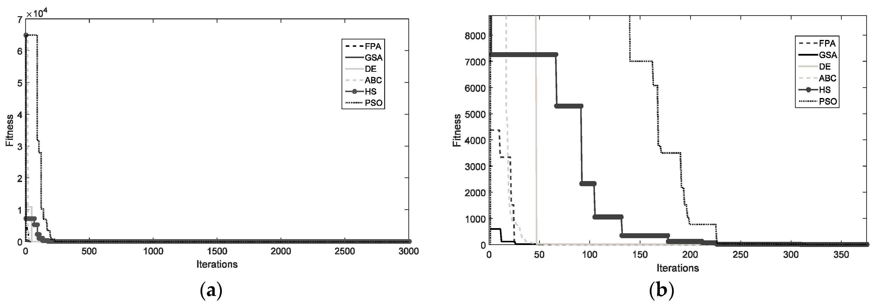
4.2. Convergence Analysis
The comparative study of the final
values cannot effectively represent the searching capabilities of the EC techniques. Hence, in
Figure 3, a convergence experiment on the seven methods is carried out. The main idea with this test is evaluating the velocity with which a compared technique approaches the optimum solution. In the test, the performance of each employed technique is examined over the minimization of the filter design. The graphs of
Figure 3 represent the median final result considering 250 executions, where each execution contemplates 3000 iterations. In the
Figure 3, it is clear that PSO and GSA converge faster than the other algorithms, but prematurely.
4.3. Computational Cost
In this experiment, the objective is to measure the number of function evaluations (
NFE) and the computing time (
CT) spent by each method required to calculate the parameters of a certain filter. All experiments consider the filter design formulated by Equations (32) and (34), which correspond to the parameters exhibited in
Table 2.
The index
NFE refers to the number of required function evaluations from which improvement is not detected in the objective function
(Equation (34)). CT represents the elapsed time in seconds consumed by each algorithm corresponding to the
NFE. The test has been executed in Matlab running on a Computer Nitro, Core i7.
Table 3 shows the averaged measurements as they are obtained from 20 independent executions. A close inspection of
Table 3 demonstrates that PSO and HS are the fastest methods. Nevertheless, this apparent velocity corresponds to premature convergence. ABC, DE and GSA are the slowest algorithms. On the other hand, FPA represents the scheme which obtains the best trade-off between velocity and accuracy.
4.4. Comparison with Different Bandwidth Sizes
In order to extend the comparison analysis, the performance of each method in the design of a low pass filter with different bandwidth sizes is evaluated. For this experiment, two particular cases are considered. In the first case, the objective is to design a filter with an ideal response defined by:
The second case considers the design of a filter with an ideal response defined as follows:
Assuming
and
as the objective functions corresponding to each ideal response
and
,
Table 4 presents comparison results. They evaluate the differences between the ideal filter response and those produced by the designed filters through EC techniques for different bandwidth sizes. The
Table 4 reports minimal (
), maximal (
) and mean (
) values of
J along with their standard deviations (
) obtained for each algorithm for every case
p = 1.2. The obtained values are calculated from 250 different executions of each method. A close inspection of
Table 4 shows that the FPA scheme produces the best performance for both cases
and
.
4.5. Filter Performance Characteristics
In this subsection, the performance of the filter characteristics is analyzed. The objective is to evaluate the responses of each of the best filters produced by every algorithm PSO, ABC, DE, HS, GSA and FPA (reported in
Table 2).
The responses are assessed considering the following indexes: (a) error in the passband, (b) magnitude ripple, (c) stop-band attenuation and (d) the magnitude of poles.
(a) Pass-band error. It evaluates the error in frequency within the passband according to the following formulation:
where
corresponds to the passband frequency.
(b) Ripple magnitude in the passband. It considers the ripple size considering the model below:
(c) The attenuation in the stop-band. It describes the response debilitation within the stop-band according to:
where
represents the stop-band frequency.
(d) The maximal pole size (MPs). This index evaluates the maximal magnitude of poles present in .
The error produced by the frequency response in the passband
corresponds to the mismatch between the transfer function of the synthesized filter
and the desired transfer function
, which models the ideal filter response. Under these conditions, a passband error as small as possible characterizes a better filter response. On the other hand, the ripple magnitude in passband
has to maintain a small enough value to guarantee lower distortions in the passband behavior. Conversely, the attenuation
should be large with the objective to eliminate undesired components of high frequency.
Table 5 presents the performance comparison of the filter characteristics. The results correspond to the responses of each of the best filters produced by each algorithm PSO, ABC, DE, HS, GSA and FPA (reported in
Table 2). On close inspection of
Table 5, it is evident that the FPA algorithm archives the best performance in error terms in passband, magnitude ripple, stop-band attenuation and magnitude of poles.
4.6. Statistical Non-Parametrical Analysis
To statistically verify the results provided by the six techniques, a nonparametric statistical significance analysis is implemented. This statistical analysis is known as Wilcoxon’s rank-sum test [
26,
28,
46,
47]. To make use of this analysis, 35 different executions for each algorithm were needed to prove that there is a significant statistical difference between the
values produced by each technique. The Wilcoxon’s rank-sum analysis provides estimating result variations between two related techniques. The study is conducted considering a 5% significance value (0.05) over the
data. Being the ABC and FPA, the techniques that better perform (according to
Table 1), we proceed to compare them with the rest of the methods.
Table 6 summarizes the
p-values performed by Wilcoxon’s analysis for the pair-wise comparison among FPA vs. PSO, FPA vs. ABC, FPA vs. DE, FPA vs. HS, FPA vs. GSA.
Table 7 reports the results among ABC vs. PSO, ABC vs. DE, ABC vs. HS, ABC vs. FPA. In the case of PSO, DE, HS and GSA, the non-parametric analysis was not conducted since the results obtained by these techniques are worse than ABC and FPA. In the Wilcoxon study, it is contemplated as the null hypothesis that there is no important difference between the two techniques. On the other hand, the alternative hypothesis is that the difference between the two approaches is important. To simplify the study of
Table 6 and
Table 7, the symbols ▲, ▼, and ► are chosen. ▲ symbolizes that the proposed approach achieves significantly better results than the compared algorithm on a specified function. ▼ expresses that the proposed approach achieves worse results than the compared technique, and ► indicates that the Wilcoxon analysis is not able to distinguish between the results of the proposed approach and the tested technique. From
Table 6 and
Table 7, it is visible that all
p-values are less than 0.05, which means that the FPA performs better than the rest of the algorithms.
Since we have run several Wilcoxon’s rank-sum tests, the probability of committing an error type 1 (false positive) increases and we can reject the null hypothesis even when it is true. To avoid this problem, a correction for the
p-values of the Wilcoxon test is adjusted by using the Bonferroni correction method [
48,
49]. Combining the Wilcoxon test with the Bonferroni method, we can show that there exists a significant statistical difference between FPA and each of the selected algorithms. The results of Bonferroni correction for FPA and ABC are shown in
Table 8 and
Table 9, respectively. The significance value of Bonferroni correction was set to
p = 0.001428 for the case of FPA comparison, and for the ABC comparison the value of Bonferroni has been set to
p = 0.000084034. It is important to point out that the absolute values of the correction factors in Bonferroni are not used for comparative proposes. In the Bonferroni test, if the new significance value is marked with 1, it means that this element confirms the result of the Wilcoxon analysis for this particular case.
4.7. Comparison Study in Images
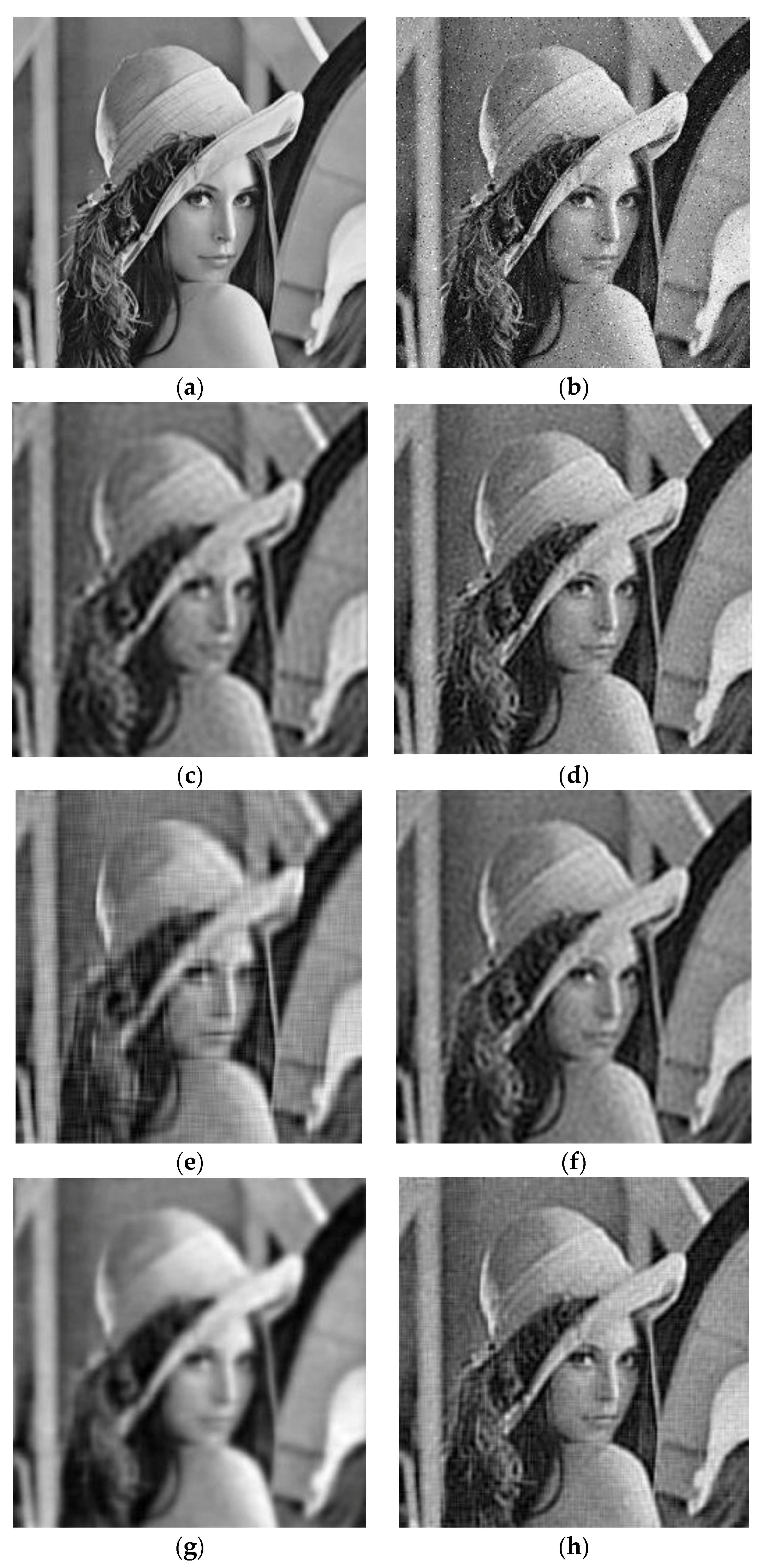
Figure 4 and
Figure 5 present the visual performance of the designed filters when they are applied to eliminate Gaussian noise for two different images.
Figure 4 shows the noise removing the results of the filters whose corresponding parameters are exhibited in
Table 2. They have been designed through the use of PSO, ABC, DE, HS, GSA and FPA considering the approximation to an ideal low pass behavior. The visual results reflex the capacity of each filter to remove noise.
Figure 4a presents the original image “Lenna”.
Figure 4b shows the image corrupted with Gaussian noise of mean = 0 and variance of 0.005. The set of images from
Figure 4c–h exhibits the performance of each method PSO, ABC, DE, HS, GSA and FPA in the noise removing process. According to the
Figure 4, it is clear that the filters produced by the FPA and ABC algorithms present the best performance. On the other hand, the filters generated by the algorithms PSO, DE, HS and GSA obtain the worst filtering effect. They are not able to remove appropriately, also producing distortions in the image due to the frequency ripples.
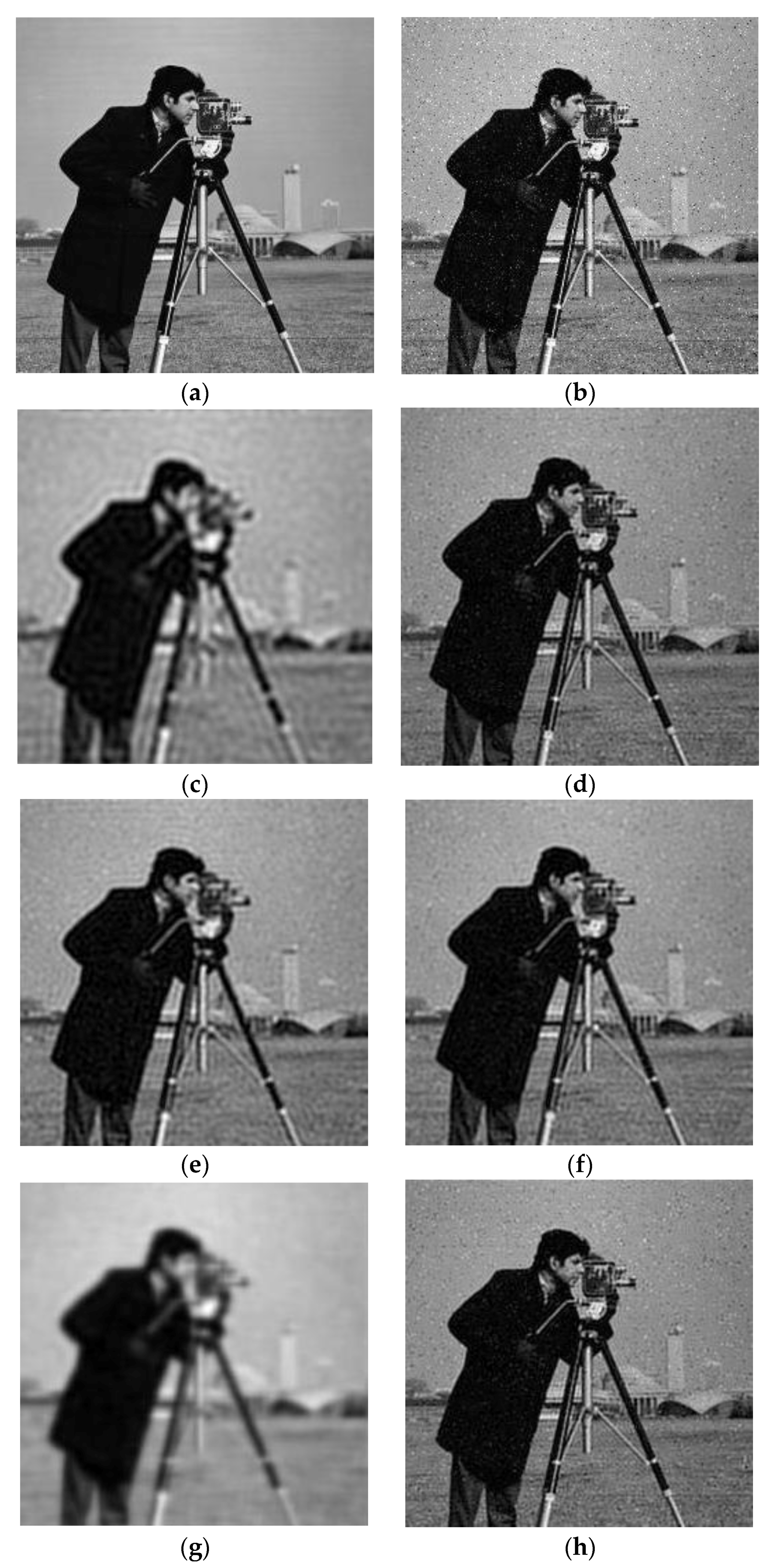
Figure 5 shows the noise removing the results of the filters with a wider bandwidth size. They correspond to the filters produced by the methods PSO, ABC, DE, HS, GSA and FPA, considering as ideal response that defined by
.
Figure 5a presents the original image “Cameraman”.
Figure 5b shows the image corrupted with Gaussian noise of mean = 0 and variance of 0.005. The set of images from
Figure 5c–h exhibits the performance of each method PSO, ABC, DE, HS, GSA and FPA in the noise removal process. Also, in this case, the filters produced by the FPA and ABC algorithms present the best noise removal result. Contrarily, the filters obtained by the algorithms PSO, DE, HS and GSA produce a bad filtering effect.
5. Discussion
The performance of EC methods is based on the balance achieved by two search procedures, namely, exploration and exploitation. In the exploration procedure, the search mechanism of EC algorithms allows producing large movements within the search space, increasing the possibility of finding potential zones. As a counterpart, the exploitation procedure increases the population diversity within the discovered zones by the exploration stage, producing better and more accurate solutions. Additionally, to know the advantages and limitations of EC methods, their correct evaluation is an important task in the computational intelligence community. In general, EC algorithms are complex pieces of software with several operators and stochastic branches. Under such circumstances, appropriate statistical methods must be considered for obtaining significant conclusions.
In this paper, a comparison study among several EC methods is conducted for solving the 2D-IIR filter design optimization problem. The experimental study compares commonly used EC methods for solving complex optimization methods. From the results, it is quite evident that the GSA algorithm is capable of producing better results than PSO, DE and HS. However, the FPA overcomes the GSA method due to the valuable combination of Lévy flights in its global pollination structure and the local pollination procedure. It can be demonstrated that for most of the experiments, FPA can be used as an alternative method for solving 2D-IIR filters.
The performance results obtained by FPA outperform the PSO, DE, HS, and GSA concerning the average and standard deviation of the values after 250 individual executions. On the other hand, the ABC overcomes the FPA in standard deviation terms, which means that ABC can converge to almost the same solution with low variation, which indicates that FPA and ABC are good alternatives for this specific application. In the case of PSO, DE, HS and GSA the fitness values obtained by these techniques were oscillatory, showing they were not able to perform the 2D-IIR filter design well.
To validate the performance results based on the minimization process, a non-parametric test known as Wilcoxon’s rank-sum was conducted. In this study, the significance level of 0.05 has been chosen, to prove if there is a statistical difference among the fitness values achieved by FPA and its competitors. Additionally, to avoid type 1 error, the Bonferroni correction has been computed to avoid false-positive results. From the statistical results, the significant performance of FPA is achieved by the balance between the global and local pollination operators.
6. Conclusions
Recently, the design of two-dimensional Infinite Impulse Response (2D-IIR) has attracted attention in several areas of engineering due to its wide range of applications. Most of the related literature concerning the optimal design of 2D-IIR structure is based on traditional optimization methods that are prone to fail in the presence of multiple optima. Under such circumstances, the optimal design of 2D-IIR filters is considered as a complex optimization problem involving multimodal surfaces.
On the other hand, Evolutionary Computation (EC) algorithms are considered as stochastic global search methods that can operate under complex multimodal error surfaces. This paper reports a comparative study considering several EC methodologies when they are applied to the complex application of 2D-IIR filter design. In comparison, special attention is paid to the most popular EC algorithms currently in use such as Particle Swarm Optimization (PSO), Artificial Bee Colony (ABC), Differential Evolution (DE), Harmony Search (HS), Gravitational Search Algorithm (GSA) and Flower Pollination Algorithm (FPA).
From the experimental results, it can be shown that the FPA method outperforms the rest of the EC techniques in terms of accuracy, consistency and robustness. Additionally, the remarkable performance of the FPA is statistically compared against the performance of its competitors considering a non-parametric test and a type 1 error correction based on a Bonferroni correction to avoid false-positive solutions. From the statistical tests, it can be corroborated that the FPA can find the optimal structure for the 2D-IIR filter design optimization problem.


