Improving the Representativeness of a Simple Random Sample: An Optimization Model and Its Application to the Continuous Sample of Working Lives

 ,
,  ,
, 

Abstract
:1. Introduction
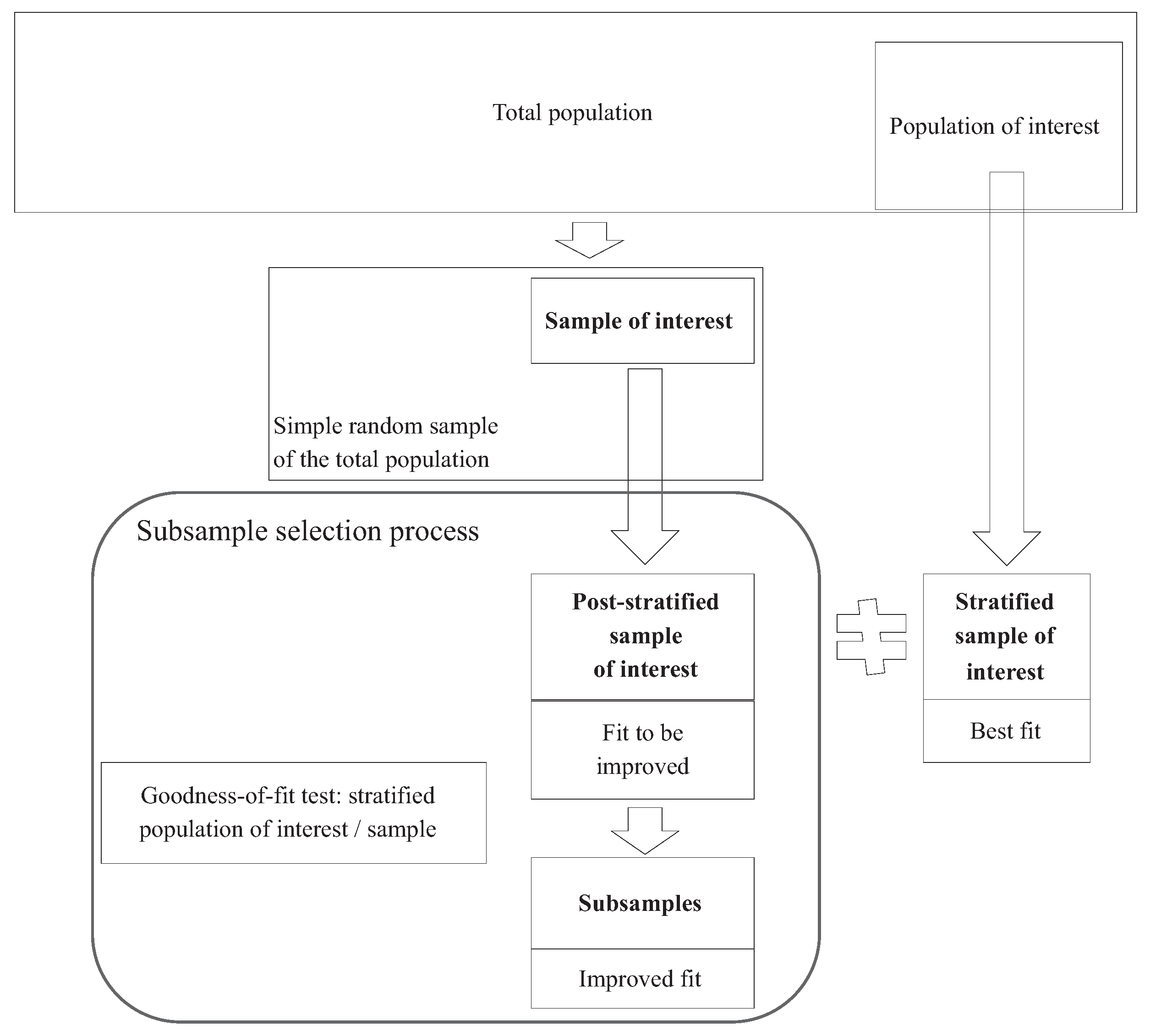
2. The Optimization Model for Improving the Representativeness of a Simple Random Sample
- The subsample must be as large as possible. We do not want to lose valuable information during the selection process, so we need to keep as many records as possible.
- The subsample must form part of both the target population and the original simple random sample. This sounds an obvious requirement, but constraints need to be included so as to avoid outliers.
- The elements to be included in each stratum of the subsample must take the form of a natural number (i.e., a non-negative integer).
- The fit or representativeness with regard to the population under study must be improved. The optimization model should therefore include a goodness-of-fit test for the distribution by strata. It should also make it a requirement that the value of the statistic is smaller than the critical value given a predetermined significance level so as to avoid rejecting the null hypothesis that the subsample has the same distribution as the population of interest. We use Pearson’s goodness-of-fit test with the test statistic:where the are the observed values (those chosen from the simple random sample to build the subsample), and the are the expected or theoretical values (those obtained from the distribution of the population of interest) and k is the number of strata for the variable of interest.
2.1. The Optimization Model
3. The Algorithm for Solving the Model and Some Simulation Results
- Preliminary: We verify that the null hypothesis of the chi-square goodness-of fit test ()—i.e., that the original simple random sample has the same distribution as the target population—is rejected. If not, we would not need to proceed. It is worth mentioning here that Pearson’s chi-square depends on the size of the sample, so the impact of effect size on the rejection of the null hypothesis has to be taken into account (see [26,27,28]). Increasing emphasis has been placed on the use of effect size reporting when analyzing social science data.To carry out this preliminary goodness-of fit test, we have to:
- Introduce the data (Input) from the target population, from the simple random sample, and set the chosen that will be the significance level for the test.
- Compute the initial values (output): size of the target population, N; size of the original simple random sample, ; expected values, , given by (14); degrees of freedom, r; and initial value of the constant of proportionality, , .
- Computing the observed values obtained by stratified sampling. Using the value for the constant of proportionality, q, which in the first iteration of the algorithm is equal to the ratio between the size of the simple random sample and the size of the target population, , we calculate the size of each stratum in the subsample using the nearest integer of as in (12), . The observed values obtained will be the same as those obtained using stratified random sampling from the target population with constant of proportionality q.
- Fitting the observed values. We compare the observed values obtained by stratified random sampling with proportional allocation from the target population, , which were found in the previous step, with those in the original simple random sample, , using (13). If , we choose for the subsample instead of the observed value obtained using from the previous step. However, if , then we take the observed value for the subsample to be , as obtained in the previous step.
- Fitting the expected values. After fitting the observed values, we calculate the total size of the subsample by adding up the number of units along the k strata, . We then compute the expected values as in order to obtain the same sum when adding up the expected values as we obtained with the observed values. If any stratum is found to be smaller than the minimum required by the test, which is usually 5, we will add it to the smallest nearest one until we reach the minimum number of elements. For Pearson’s chi-square goodness-of-fit test to be valid, the sample size must be large enough to provide a minimum number of expected elements per category. Núñez-Antón, Pérez-Salamero González, Regúlez-Castillo, Ventura-Marco, and Vidal-Meliá [30] have developed functions for regrouping strata automatically no matter where they are located, thus enabling the goodness-of-fit test to be performed within an iterative procedure. The functions are written in Excel VBA (Visual Basic for Applications 7.1) and Mathematica, a registered trademark of Wolfram Research Inc. version 11.
- Goodness-of-fit test. Using (10) and (11), we now test the null hypothesis, —i.e., that the subsample has the same distribution as the target population—by comparing the fitted observed values with the fitted expected values obtained in steps 2 and 3 above. If the null hypothesis is not rejected, we can stop the algorithm because we have found the optimal , i.e., the distribution of the largest subsample contained in the original simple random sample that fits the population of interest. If the null hypothesis is rejected, we will proceed to the next step.
- New value of q. To find the new value of q in order to start the process again, we now aim to obtain a reduction of q, requiring that will provide the global optimal solution. The new value of , , used to start iteration j, is obtained by subtracting from the previous constant of proportionality, , a step value () that is obtained in each case from the initial value of the constant of proportionality:To shorten the time taken to find the solution, we incrementally reduce q as much as possible to the point where it does not reject the null hypothesis in the goodness-of-fit test. We then reverse the process in order to consider the immediately preceding value of . From that value onwards, we are conducting a grid search in a finer set.
- The number of strata is a random integer number between 2 and 20.
- The 4000 populations are generated in four blocks of 1000 as a function of the maximum size of the population strata—1000, 10,000, 100,000, and 1,000,000—given that the minimum size is 1 for all cases.
- The size of the simple random sample stratum is an integer number that results from rounding the product of the size of the corresponding stratum in the population by a percentage. This percentage is randomly selected from an interval that we have set to be for the “bad” fit and for the “fine” fit.
- For the 4000 simulations in each group, the optimization model is solved by means of our proposed algorithm with a given significance level, , of , which is the most common significance level in practice. The optimization model was solved using MsExcel Professional Plus 2016, VBA 7.1, in a computer with an Intel Core i7-2600 Quad-Core Processor 3.4 GHz, 32 GB RAM and a Windows 7 Enterprise 64-bit system.
4. Applying the Model to the Continuous Sample of Working Lives (CSWL)
The Optimization Model Adapted to the CSWL
- : the size of the subsample.
- : the size of the stratum i, j, k in the target population. It is the number of pensioners in the population, with the sub-indices representing the corresponding groups by age, gender, and type of benefit. These data are obtained from INSS [99].
- : the total number of beneficiaries. These data are obtained from INSS [99].
- : the size of the stratum i, j, k in CSWL. It is the number of pensioners in CSWL, with the sub-indices representing the corresponding groups by age, gender, and type of benefit.
- : the size of the CSWL.
- : the expected size of stratum i,j,k in the subsample. This depends on the population relative frequency and the size of the subsample .
- : the size of the stratum i, j, k in the subsample (observed values).
- : a function that returns the nearest integer to its argument.
- : the expected size of the regrouped stratum i, j, k in the subsample.
- : the size of the regrouped stratum i, j, k in the subsample (observed values).
- : a function that depends on the chi-square statistic and the degrees of freedom, both of which in the end also depend on the constant of proportionality and, above all, the values estimated and observed after regrouping (where applicable).
- : the sample value for the chi-square statistic calculated in each iteration for each gender and type of pension (ten cases, i.e., five types of pension/2 genders). It evaluates the difference between the regrouped observed values and the expected values for cohort indices with five or more elements, avoiding those indices in which the regrouped cohort has no elements.
- : a function that returns the degrees of freedom in each iteration once the goodness-of-fit test is calculated for each type of pension and gender. It is equal to the expected number of regrouped cohorts minus 1, given that there are no parameters to estimate because the population distribution is already known.
- : a pre-established level of statistical significance which is the criterion for the subsample to improve the goodness of fit to the population. This pre-established minimum p-value will be the same for all ten cases (five types of pension/2 genders) and has to be high in order to guarantee a better fit to the population than the value given by the CSWL.
- : a set of indices for regrouped age cohorts that contain five or more elements, for each type of pension and gender.
- : a set of indices for age cohorts by type of pension and gender, which in all cases has 18 age cohorts.
5. Main Results
6. Discussion
Author Contributions
Funding
Acknowledgments
Conflicts of Interest
Appendix A. Nomenclature Chapter
- : the size of stratum i in the subsample (observed values).
- : the size of the subsample.
- : the expected size of stratum i in the subsample. This depends on the population relative frequency and the size of the subsample .
- : the size of the stratum i in the target population.
- N: the size of the target population.
- : the size of stratum i in the simple random sample.
- : the size of the simple random sample.
- : the chi-square goodness-of-fit test statistic.
- : the tabulated value of the chi-square distribution with r degrees of freedom and a significance level equal to .
- k: the number of strata for the variable of interest.
- : the degrees of freedom equal to the number of strata minus 1, given that in this case there are no parameters to be estimated because the population distribution is known.
- Z: the set of integer numbers.
- : function that rounds its argument to the nearest integer.
- : the size of the subsample.
- : the expected size of stratum i in the subsample. This depends on the population relative frequency and the size of the subsample .
- k: the number of strata for the variable of interest.
- : the size of the stratum i in the target population.
- N: the size of the target population.
- : the size of stratum i in the simple random sample.
- : the chi-square goodness-of-fit test statistic.
- : the degrees of freedom equal to the number of strata minus 1, given that in this case there are no parameters to be estimated because the population distribution is known.
- : a function that calculates the p-value given the value of the test statistic, and the degrees of freedom, r, as in (8).
- : a pre-established level of statistical significance which is the criterion for the subsample to improve the goodness of fit to the population.
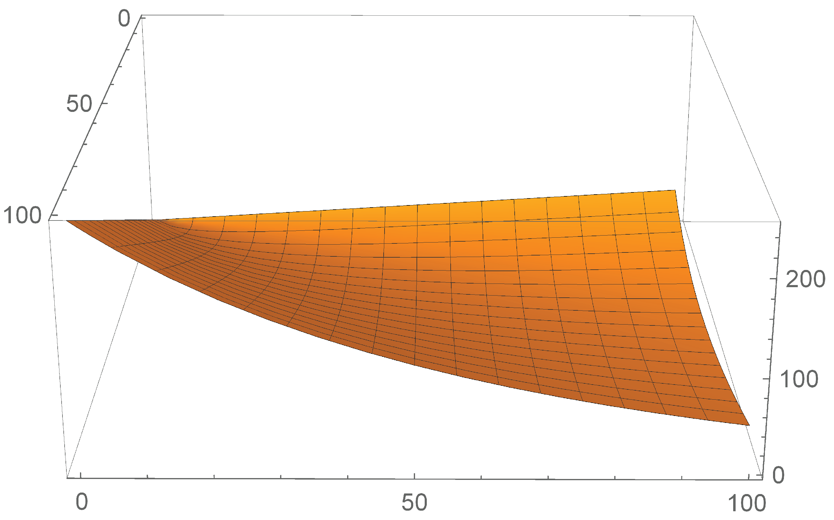
Appendix B. Proof of the Convexity of the Chi-Square Statistic Function in


References
- Ramsey, C.A.; Hewitt, A.D. A methodology for assessing sample representativeness. Environ. Forensics 2005, 6, 71–75. [Google Scholar] [CrossRef]
- Grafstrom, A.; Schelin, L. How to select representative samples. Scand. J. Stat. 2014, 41, 277–290. [Google Scholar] [CrossRef]
- Kruskall, W.; Mosteller, F. Representative sampling, I. Int. Stat. Rev. 1979, 47, 13–24. [Google Scholar] [CrossRef]
- Kruskall, W.; Mosteller, F. Representative sampling, II: Scientific literature, excluding statistics. Int. Stat. Rev. 1979, 47, 111–127. [Google Scholar] [CrossRef]
- Kruskall, W.; Mosteller, F. Representative sampling, III: The current statistical literature. Int. Stat. Rev. 1979, 47, 245–265. [Google Scholar] [CrossRef]
- Kruskall, W.; Mosteller, F. Representative sampling, IV: The history of the concept in statistics, 1895–1939. Int. Stat. Rev. 1980, 48, 169–195. [Google Scholar] [CrossRef]
- Omair, A. Sample size estimation and sampling techniques for selecting a representative sample. J. Health Spec. 2014, 2, 142–147. [Google Scholar] [CrossRef]
- Bonami, P.; Kilinç, M.; Linderoth, J. Algorithms and software for convex mixed integer nonlinear programs. In Mixed Integer Nonlinear Programming. The IMA Volumes in Mathematics and its Applications; Lee, J., Leyferr, S., Eds.; Springer: New York, NY, USA, 2012; Volume 154, pp. 1–39. [Google Scholar]
- D’Ambrosio, C.; Lodi, A. Mixed integer nonlinear programming tools: An updated practical overview. Ann. Oper. Res. 2013, 204, 301–320. [Google Scholar] [CrossRef]
- MESS: Documentación Muestra Continua de Vidas Laborales: MCVL Guía. Madrid: Secretaría de Estado de la Seguridad Social. Ministerio de Trabajo, Migraciones y Seguridad Social. Available online: http://www.seg-social.es/ (accessed on 12 March 2020).
- Pérez-Salamero González, J.M.; Regúlez-Castillo, M.; Vidal-Meliá, C. Análisis de la representatividad de la MCVL: El caso de las prestaciones del sistema público de pensiones. Hacienda Pública Esp. 2016, 217, 67–130. [Google Scholar] [CrossRef] [Green Version]
- Pérez-Salamero González, J.M.; Regúlez-Castillo, M.; Vidal-Meliá, C. The continuous sample of working lives: Improving its representativeness. SERIEs 2017, 8, 43–95. [Google Scholar] [CrossRef] [Green Version]
- Cochran, W.G. Sampling Techniques; Wiley: New York, NY, USA, 1977. [Google Scholar]
- Särndal, C.E.; Swensson, B.; Wretman, J. Model Assisted Survey Sampling. Springer Series in Statistics; Springer: New York, NY, USA, 1992. [Google Scholar]
- Valliant, R.; Gentle, J.E. An application of mathematical programming to sample allocation. Comput. Stat. Data An. 1997, 25, 337–360. [Google Scholar] [CrossRef]
- Baillargeon, S.; Rivest, L.P. A general algorithm for univariate stratification. Int. Stat. Rev. 2009, 77, 331–344. [Google Scholar] [CrossRef]
- Díaz-García, J.A.; Ramos-Quiroga, R. Optimum allocation in multivariable stratified random sampling: Stochastic matrix mathematical programming. Stat. Neerl. 2012, 66, 492–511. [Google Scholar] [CrossRef]
- Gupta, N.; Sana Ifthekar, S.; Bari, A. Fuzzy goal programming approach to solve nonlinear bi-level programming problem in stratified double sampling design in the presence of non-response. Int. J. Sci. Eng. Res. 2012, 3, 1–9. [Google Scholar]
- Valliant, R.; Dever, J.; Kreuter, F. Practical Tools for Designing and Weighting Survey Samples; Springer: New York, NY, USA, 2013. [Google Scholar]
- Díaz-García, J.A.; Ramos-Quiroga, R. Optimum allocation in multivariable stratified random sampling: A modified Prékopa’s approach. J. Math. Mod. Algorithms 2014, 13, 315–330. [Google Scholar] [CrossRef]
- Gupta, N.; Ali, I.; Bari, A. An optimal chance constraint multivariate stratified sampling design using auxiliary information. J. Math. Mod. Algorithms Oper. Res. 2014, 13, 341–352. [Google Scholar] [CrossRef]
- De Moura Brito, J.A.; Do Nascimento Silva, P.L.; Silva Semaan, G.; Maculan, N. Integer programming formulations applied to optimal allocation in stratified sampling. Surv. Methodol. 2015, 41, 427–442. [Google Scholar]
- Neyman, J. On the two different aspects of the representative method: The method of representative sampling and the method of purposive sampling. J. R. Stat. Soc. 1934, 97, 558–625. [Google Scholar] [CrossRef]
- Kontopantelis, E. A greedy algorithm for representative sampling: Repsample in Stata. J. Stat. Softw. 2013, 56, 1–18. [Google Scholar]
- Bowley, A.L. Measurement of precision attained in sampling. B. Int. Statist. Inst. 1926, 22, 6–62. [Google Scholar]
- Berkson, J. Some difficulties of interpretation encountered in the application of the chi-square test. J. Am. Stat. Assoc. 1938, 33, 526–536. [Google Scholar] [CrossRef]
- Wang, C. Sense and Nonsense of Statistical Inference: Controversy, Misuse and Subtlety; Marcel Dekker: New York, NY, USA, 1993. [Google Scholar]
- Lin, M.; Lucas, H.C.; Shmieli, G. Research commentary: Too big to fail: Large samples and the p-value problem. Inform. Syst. Res. 2013, 24, 906–917. [Google Scholar] [CrossRef] [Green Version]
- Cohen, J. Statistical Power Analysis for the Behavioral Sciences; Erlbaum: Hillsdale, NJ, USA, 1988. [Google Scholar]
- Núñez-Antón, V.; Pérez-Salamero González, J.M.; Regúlez-Castillo, M.; Ventura-Marco, M.; Vidal-Meliá, C. Automatic regrouping of strata in the goodness-of-fit chi-square test. SORT 2019, 43, 113–142. [Google Scholar]
- DGOSS: Muestra Continua de vidas Laborales, 2005–2017. Madrid: Secretaría de Estado de la Seguridad Social. Ministerio de Trabajo, Migraciones y Seguridad Social. Available online: http://www.seg-social.es/wps/portal/wss/internet/EstadisticasPresupuestosEstudios/Estadisticas/ (accessed on 12 March 2020).
- Agliari, E.; Barra, A.; Contucci, P.; Sandell, R.; Vernia, C. A stochastic approach for quantifying immigrant integration: The Spanish test case. New J. Phys. 2014, 16. [Google Scholar] [CrossRef] [Green Version]
- Barra, A.; Contucci, P.; Sandell, R.; Vernia, C. An analysis of a large dataset on immigrant integration in Spain. The statistical mechanics perspective on social action. Sci. Rep. 2014, 4, 4174. [Google Scholar] [CrossRef] [PubMed] [Green Version]
- Carrasco, R.; García Pérez, J.I. Employment dynamics of immigrants versus natives: Evidence from the boom-bust period in Spain, 2000–2011. Econ. Inq. 2015, 53, 1038–1060. [Google Scholar] [CrossRef] [Green Version]
- De Pedraza, P.; Villacampa González, A.; Muñoz de Bustillo Llorente, R. Immigrants’ employment situations and decent work determinants in the Spanish labour market. Int. J. Humanit. Soc. Sci. 2012, 2, 1–19. [Google Scholar]
- Gómez Tello, A.; Nicolini, R. Immigration and productivity: A Spanish tale. J. Prod. Anal. 2017, 47, 167–183. [Google Scholar] [CrossRef] [Green Version]
- González, L.; Ortega, F. How do very open economies adjust to large immigration flows? Evidence from Spanish regions. Labour Econ. 2011, 18, 57–70. [Google Scholar] [CrossRef]
- Solé, M.; Díaz Serrano, L.; Rodríguez, M. Disparities in work, risk and health between immigrants and native-born Spaniards. Soc. Sci. Med. 2013, 76, 179–187. [Google Scholar] [CrossRef] [Green Version]
- Alonso Domínguez, A. Labor transitions of Spanish workers: A flexicurity approach. Rev. Int. Org. 2012, 9, 121–143. [Google Scholar]
- Álvarez de Toledo, P.; Núñez, F.; Usabiaga, C. An empirical analysis of the matching process in Andalusian public employment agencies. Hacienda Pública Esp. 2011, 198, 67–102. [Google Scholar]
- Álvarez de Toledo, P.; Núñez, F.; Usabiaga, C. An empirical approach on labour segmentation. Applications with individual duration data. Econ. Model. 2014, 36, 252–267. [Google Scholar] [CrossRef]
- Álvarez de Toledo, P.; Núñez, F.; Usabiaga, C. ¿Quién se empareja con quién en el mercado laboral español? Un análisis clúster basado en la muestra continua de vidas laborales. Investigación Económica 2017, 76, 3–182. [Google Scholar]
- Álvarez de Toledo, P.; Núñez, F.; Usabiaga, C. Análisis “cluster” de los flujos laborales andaluces. Rev. Estud. Reg. 2013, 97, 195–221. [Google Scholar]
- Cueto, B.; Rodríguez, V. Sheltered employment centres and labour market integration of people with disabilities: A quasi-experimental evaluation using Spanish data. In Disadvantaged Workers. Empirical Evidence and Labour Policies; Malo, M., Sciulli, D., Eds.; Springer: New York, NY, USA, 2014; pp. 65–91. [Google Scholar]
- García Pérez, J.I.; Marinescu, I.; Castelló, J.V. Can fixed-term contracts put low skilled youth in a better career path? Evidence from Spain. Econ. J. 2019, 129, 1693–1730. [Google Scholar] [CrossRef] [Green Version]
- García Pérez, J.I.; Osuna, V. Dual labour markets and the tenure distribution: Reducing severance pay or introducing a single contract? Labour Econ. 2014, 29, 1–13. [Google Scholar] [CrossRef]
- García Pérez, J.I.; Rebollo Sanz, Y. The use of permanent contracts across Spanish regions: Do regional wage subsidies work? Investig. Econ. 2009, 33, 97–130. [Google Scholar]
- Garda, P. Essays on the Macroeconomics of Labor Markets. Ph.D. Dissertation, Universitat Pompeu Fabra, Barcelona, Spain, 2013. [Google Scholar]
- Úbeda, M.; Cabasés, M.Á.; Sabaté, M.; Strecker, T. The Deterioration of the Spanish Youth Labour Market (1985–2015): An Interdisciplinary Case Study. YoUnG 2020. [Google Scholar] [CrossRef]
- Vall Castelló, J. Promoting employment of disabled women in Spain: Evaluating a policy. Labour Econ. 2012, 19, 82–91. [Google Scholar] [CrossRef] [Green Version]
- Vall Castelló, J. What happens to the employment of disabled individuals when all financial disincentives to work are abolished? Health Econ. 2017, 26, 158–174. [Google Scholar] [CrossRef] [Green Version]
- Alonso, F.; Devesa, J.E.; Devesa, M.; Domínguez, I.; Encinas, B.; Meneu, R.; Nagore, A. Towards an adequate and sustainable replacement rate in defined benefit pension systems: The case of Spain. Int. Soc. Secur. Rev. 2018, 71, 51–70. [Google Scholar] [CrossRef] [Green Version]
- Boado-Penas, M.C.; Valdés-Prieto, S.; Vidal-Meliá, C. An actuarial balance sheet for pay-as-you-go finance: Solvency indicators for Spain and Sweden. Fisc. Stud. 2008, 29, 89–134. [Google Scholar] [CrossRef] [Green Version]
- Conde Ruiz, J.I.; González, C.I. Reforma de pensiones 2011 en España. Hacienda Pública Esp. 2013, 204, 9–44. [Google Scholar]
- Conde-Ruiz, J.I.; González, C.I. From Bismarck to Beveridge: The other pension reform in Spain. SERIEs 2016, 7, 461–490. [Google Scholar] [CrossRef] [Green Version]
- Devesa, J.E.; Devesa, M.; Domínguez, I.; Encinas, B.; Meneu, R.; Nagore, A. Equidad y sostenibilidad como objetivos ante la reforma del sistema contributivo de pensiones de jubilación. Hacienda Pública Esp. 2012, 201, 9–38. [Google Scholar]
- García García, M.; Nave Pineda, J.M. Impacto en las prestaciones de jubilación de la reforma del sistema público de pensiones español. Hacienda Pública Esp. 2018, 224, 113–137. [Google Scholar] [CrossRef]
- Moral Arce, I.; Patxot, C.; Souto, G. La sostenibilidad del sistema de pensiones. Una aproximación a partir de la CSWL. Revista de Economía Aplicada 2008, 16, 29–66. [Google Scholar]
- Muñoz de Bustillo, R.; De Pedraza, P.; Antón, J.I.; Rivas, L.A. Working life and retirement pensions in Spain: The simulated impact of a parametric reform. Int. Soc. Secur. Rev. 2011, 64, 73–93. [Google Scholar] [CrossRef]
- Patxot, C.; Souto, G.; Villanueva, J. Fostering the contributory nature of the Spanish retirement pension system: An arithmetic micro-simulation exercise using the MCVL. Presup. Gasto Público 2009, 57, 7–32. [Google Scholar]
- Peinado Martínez, P. Pension System’s reform in Spain: A dynamic analysis of the effects on welfare. Ph.D. Dissertation, Universidad del País Vasco UPV/EHU, Bilbao, Spain, 2011. [Google Scholar]
- Peinado Martínez, P. A dynamic gender analysis of Spain’s pension reforms of 2011. Fem. Econ. 2014, 20, 163–190. [Google Scholar] [CrossRef]
- Peinado Martínez, P.; Serrano Pérez, F. A dynamic analysis of the effect of social security reform on Spanish widow pensioners. Panoeconomicus 2011, 58, 759–771. [Google Scholar] [CrossRef]
- Sánchez Martín, A.R.; Sánchez Marcos, V. Demographic change and pension reform in Spain: An assessment in a two-earner OLG model. Fisc. Stud. 2010, 31, 405–452. [Google Scholar] [CrossRef]
- Vidal-Meliá, C. An assessment of the 2011 Spanish pension reform using the Swedish system as a benchmark. J. Pension Econ. Financ. 2014, 13, 297–333. [Google Scholar] [CrossRef]
- Vidal-Meliá, C.; Boado Penas, M.C.; Settergren, O. Automatic balance mechanisms in pay-as-you-go pension systems. Geneva Pap. Risk Insur. Issues Pract. 2009, 34, 287–317. [Google Scholar] [CrossRef] [Green Version]
- Amuedo Dorantes, C.; Borra, C. On the differential impact of the recent economic downturn on work safety by nativity: The Spanish experience. IZA J. Dev. Migr. 2013, 2, 1–26. [Google Scholar] [CrossRef] [Green Version]
- Anghel, B.; Basso, H.; Bover, O.; Casado, J.M.; Hospido, L.; Izquierdo, M.; Kataryniuk, I.A.; Lacuesta, A.; Montero, J.M.; Vozmediano, E. Income, consumption and wealth inequality in Spain. SERIEs 2018, 9, 351–357. [Google Scholar] [CrossRef] [Green Version]
- Antón, J.I.; Muñoz, R. Public-private sector wage differentials in Spain. An updated picture in the midst of the great recession. Investigación Económica 2015, 324, 115–157. [Google Scholar] [CrossRef] [Green Version]
- Dudel, C.; López Gómez, M.A.; Benavides, F.G.; Myrskylä, M. The length of working life in Spain: Levels, recent trends, and the impact of the financial crisis. Eur. J. Popul. 2018, 34, 769–791. [Google Scholar] [CrossRef] [Green Version]
- Arranz, J.M.; García-Serrano, C. Are the MCVL tax data useful? Ideas for mining. Hacienda Pública Esp. 2011, 199, 151–186. [Google Scholar]
- Arranz, J.M.; García-Serrano, C.; Hernanz, V. How do we pursue “labormetrics”? An application using the MCVL. Estadística Española 2013, 55, 231–254. [Google Scholar]
- De la Roca, J.; Puga, D. Learning by working in big cities. Rev. Econ. Stud. 2017, 84, 106–142. [Google Scholar] [CrossRef]
- López, M.A.; Benavides, F.G.; Alonso, J.; Espallargues, M.; Durán, X.; Martínez, J.M. The value of using administrative data in public health research: The continuous working life sample. Gac. Sanit. 2014, 28, 334–337. [Google Scholar] [CrossRef] [PubMed] [Green Version]
- Pérez-Salamero González, J.M. La MCVL como fuente generadora de datos para el estudio del sistema de pensiones. Ph.D. Dissertation, Universidad de Valencia, Valencia, Spain, 2015. [Google Scholar]
- Arranz, J.M.; García-Serrano, C. Duration and recurrence in unemployment benefits. J. Labor Res. 2014, 35, 271–295. [Google Scholar] [CrossRef] [Green Version]
- Arranz, J.M.; García-Serrano, C. Duration of joblessness and long-term unemployment: Is duration as long as official statistics say? In Disadvantaged Workers. Empirical Evidence and Labour Policies; Malo, M., Sciulli, D., Eds.; Springer: New York, NY, USA, 2014; pp. 297–320. [Google Scholar]
- Arranz, J.M.; García-Serrano, C. The interplay of the unemployment compensation system, fixed-term contracts and rehirings: The case of Spain. Int. J. Manpower 2014, 35, 1236–1259. [Google Scholar] [CrossRef]
- Bentolila, S.; García-Pérez, J.I.; Jansen, M. Are the Spanish long-term unemployed employable? SERIEs 2017, 8, 1–41. [Google Scholar] [CrossRef] [Green Version]
- Nagore García, A. Gender differences in unemployment dynamics and initial wages over the business cycle. J. Labor Res. 2017, 38, 228–260. [Google Scholar] [CrossRef]
- Rebollo-Sanz, Y. Unemployment insurance and job turnover in Spain. Labour Econ. 2012, 19, 403–426. [Google Scholar] [CrossRef] [Green Version]
- Benavides, F.G.; Durán, X.; Gimeno, D.; Vanroelen, C.; Martínez, J.L. Labour market trajectories and early retirement due to permanent disability: A study based on 14972 new cases in Spain. Eur. J. Public Health. 2015, 25, 673–677. [Google Scholar] [CrossRef]
- Carrillo-Castrillo, J.A.; Guadix, J.; Rubio-Romero, J.C.; Onieva, L. Estimation of the Relative Risks of Musculoskeletal Injuries in the Andalusian Manufacturing Sector. Int. J. Ind. Ergonom. 2016, 52, 69–77. [Google Scholar] [CrossRef]
- Castañer-Garriga, A.; Pérez-Salamero González, J.M.; Vidal-Meliá, C. Evaluación de las tarifas de las pensiones de accidentes de trabajo y enfermedades profesionales (2011–2015). Rev. Innovar J. 2017, 27, 153–167. [Google Scholar] [CrossRef]
- Durán, X.; Vanroelend, C.; Deboosere, P.; Benavides, F.G. Social security status and mortality in Belgian and Spanish male workers. Gac. Sanit. 2016, 30, 293–295. [Google Scholar] [CrossRef] [PubMed] [Green Version]
- Jiménez-Martín, S.; Juanmartí Mestres, A.; Vall Castelló, J. Hiring subsidies for people with a disability: Do They Work? Eur. J. Health Econ. 2019, 20, 669–689. [Google Scholar] [CrossRef] [PubMed]
- López Gómez, M.A.; Serra, L.; Delclos, G.L.; Benavides, F.G. Employment history indicators and mortality in a nested case-control study from the Spanish WORKing life social security (WORKss) cohort. PLoS ONE 2017, 12, E0178486. [Google Scholar] [CrossRef] [PubMed]
- López Gómez, M.A.; Durán, X.; Zaballa, E.; Sanchez-Niubo, A.; Delclos, G.L.; Benavides, G.L. Cohort profile: The Spanish WORKing life Social security (WORKss) cohort Study. BMJ Open 2016, 6. [Google Scholar] [CrossRef] [PubMed] [Green Version]
- López, M.A.; Durán, X.; Alonso, J.; Martínez, J.M.; Espallargues, M.; Benavides, F.G. Estimating the burden of disease due to permanent disability in Spain during the period 2009–2012. Rev. Esp. Salud Public. 2014, 88, 349–358. [Google Scholar] [CrossRef] [Green Version]
- Bonhomme, S.; Hospido, L. Earnings inequality in Spain: New Evidence using tax data. Appl. Econ. 2013, 45, 4212–4225. [Google Scholar] [CrossRef]
- Bonhomme, S.; Hospido, L. The cycle of earnings inequality: Evidence from Spanish social security data. Econ. J. 2017, 127, 1244–1278. [Google Scholar] [CrossRef] [Green Version]
- Marie, O.; Vall Castelló, J. Measuring the (income) effect of disability insurance generosity on labour market participation. J. Public Econ. 2012, 96, 198–210. [Google Scholar] [CrossRef] [Green Version]
- Cairó Blanco, I. An empirical analysis of retirement behaviour in Spain: Partial versus full retirement. SERIEs 2010, 1, 325–356. [Google Scholar] [CrossRef] [Green Version]
- García-Gómez, P.; Jiménez-Martín, S.; Castelló, J.V. Health, disability, and pathways into retirement in Spain. In Social Security Programs and Retirement around the World; Wise, D.A., Ed.; University of Chicago Press: Chicago, IL, USA, 2012; pp. 127–174. [Google Scholar]
- García Pérez, J.I.; Jiménez Martín, S.; Sánchez Martín, A.R. Retirement incentives, individual heterogeneity and labor transitions of employed and unemployed workers. Labour Econ. 2013, 20, 106–120. [Google Scholar] [CrossRef]
- Vegas Sánchez, R.; Argimón, I.; Botella, M.; González, C. Old age pensions and retirement in Spain. SERIEs 2013, 4, 273–307. [Google Scholar] [CrossRef] [Green Version]
- Cebrián, I.; Moreno, G. Labour market intermittency and its effect on gender wage gap in Spain. Rev. Interv. Econ. 2013, 47. [Google Scholar] [CrossRef] [Green Version]
- Cebrián, I.; Moreno, G. The effects of gender differences in career interruptions on the gender wage gap in Spain. Fem. Econ. 2015, 21, 1–27. [Google Scholar] [CrossRef]
- INSS: Informes estadísticos, 2005–2017. Madrid: Instituto Nacional de la Seguridad Social. Secretaría de Estado de la Seguridad Social. Ministerio de Trabajo, Migraciones y Seguridad Social. Available online: http://www.mitramiss.gob.es/es/estadisticas/ (accessed on 12 March 2020).


| Cases by Maximum Strata Size | |||||||||
|---|---|---|---|---|---|---|---|---|---|
| 1000 | 10,000 | 100,000 | 1,000,000 | ||||||
| Items | Bad | Fine | Bad | Fine | Bad | Fine | Bad | Fine | |
| 1 | Simple random sample reject cases | 714 | - | 938 | 437 | 992 | 901 | 996 | 989 |
| 2 | Global solution cases with ES | 714 | - | 936 | 434 | 977 | 783 | 977 | 840 |
| 3 | Cases with regrouped stratum = 1 | 13 | - | 3 | 0 | 1 | 0 | 0 | 0 |
| 4 | Average time seconds | 3.34 | - | 23.26 | 4.19 | 50.98 | 11.21 | 101.15 | 13.89 |
| 5 | Average subsample size | 119.8 | - | 492.7 | 1696.8 | 3044.1 | 10,667.9 | 23,925.7 | 97,970.5 |
| 6 | Relative average % | 65.81 | - | 41.01 | 93.49 | 28.56 | 88.92 | 22.9 | 84.09 |
| 7 | Average | 4.64 | - | 3.39 | 1.20 | 2.02 | 1.12 | 1.32 | 1.06 |
| 8 | 306 | - | 107 | 15 | 21 | 2 | 7 | 0 | |
| 9 | Average Cramer’s V | 0.21 | - | 0.20 | 0.05 | 0.21 | 0.05 | 0.20 | 0.05 |
| 10 | Average df | 8.89 | - | 9.95 | 11.49 | 10.01 | 11.06 | 10.19 | 10.97 |
| 11 | Type of ES | Large | - | Large | Small | Large | Small | Large | Small |
| 12 | Small cases | 8 | - | 60 | 434 | 67 | 783 | 68 | 840 |
| 13 | Medium cases | 270 | - | 304 | - | 328 | - | 313 | - |
| 14 | Large cases | 436 | - | 572 | - | 582 | - | 596 | - |
| Time (sec.) | ||||||||||||||
|---|---|---|---|---|---|---|---|---|---|---|---|---|---|---|
| Year | 0.05 | 0.5 | 0.95 | 0.05 | 0.5 | 0.95 | 0.05 | 0.5 | 0.95 | 0.05 | 0.5 | 0.95 | D.I.U | Effect Size |
| 2005 | 240,702 | 227,849 | 177,856 | 2.971 | 2.812 | 2.195 | 74.65 | 70.67 | 55.16 | 5.570 | 5.180 | 8.814 | 7.188 | Medium |
| 2006 | 315,634 | 308,116 | 204,716 | 3.836 | 3.745 | 2.488 | 95.83 | 93.55 | 62.16 | 7.051 | 8.752 | 7.629 | 3.564 | Medium |
| 2007 | 319,612 | 310,649 | 300,913 | 3.835 | 3.727 | 3.610 | 96.09 | 93.40 | 90.47 | 8.439 | 4.727 | 8.222 | 7.216 | Small |
| 2008 | 329,204 | 321,031 | 311,082 | 3.887 | 3.790 | 3.673 | 97.37 | 94.95 | 92.01 | 8.939 | 7.738 | 6.864 | 6.468 | Medium |
| 2009 | 335,665 | 330,298 | 315,426 | 3.897 | 3.835 | 3.662 | 97.76 | 96.20 | 91.87 | 8.549 | 10.359 | 8.487 | 1.083 | Medium |
| 2010 | 339,831 | 335,482 | 318,778 | 3.885 | 3.835 | 3.644 | 97.33 | 96.08 | 91.30 | 7.613 | 7.191 | 5.585 | 2.204 | Medium |
| 2011 | 343,317 | 334,590 | 300,129 | 3.871 | 3.772 | 3.384 | 97.30 | 94.82 | 85.06 | 8.860 | 8.767 | 6.848 | 4.670 | Medium |
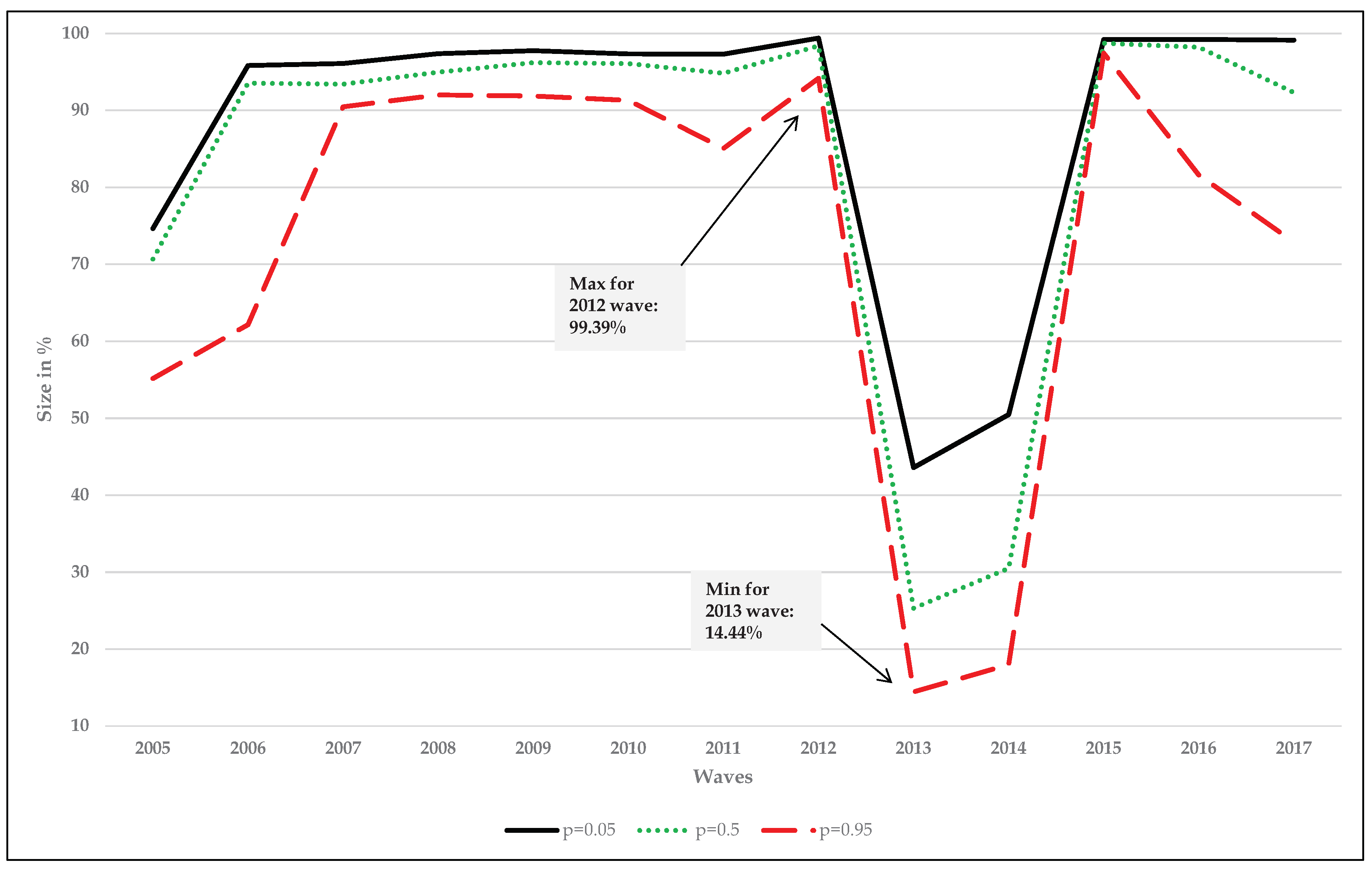
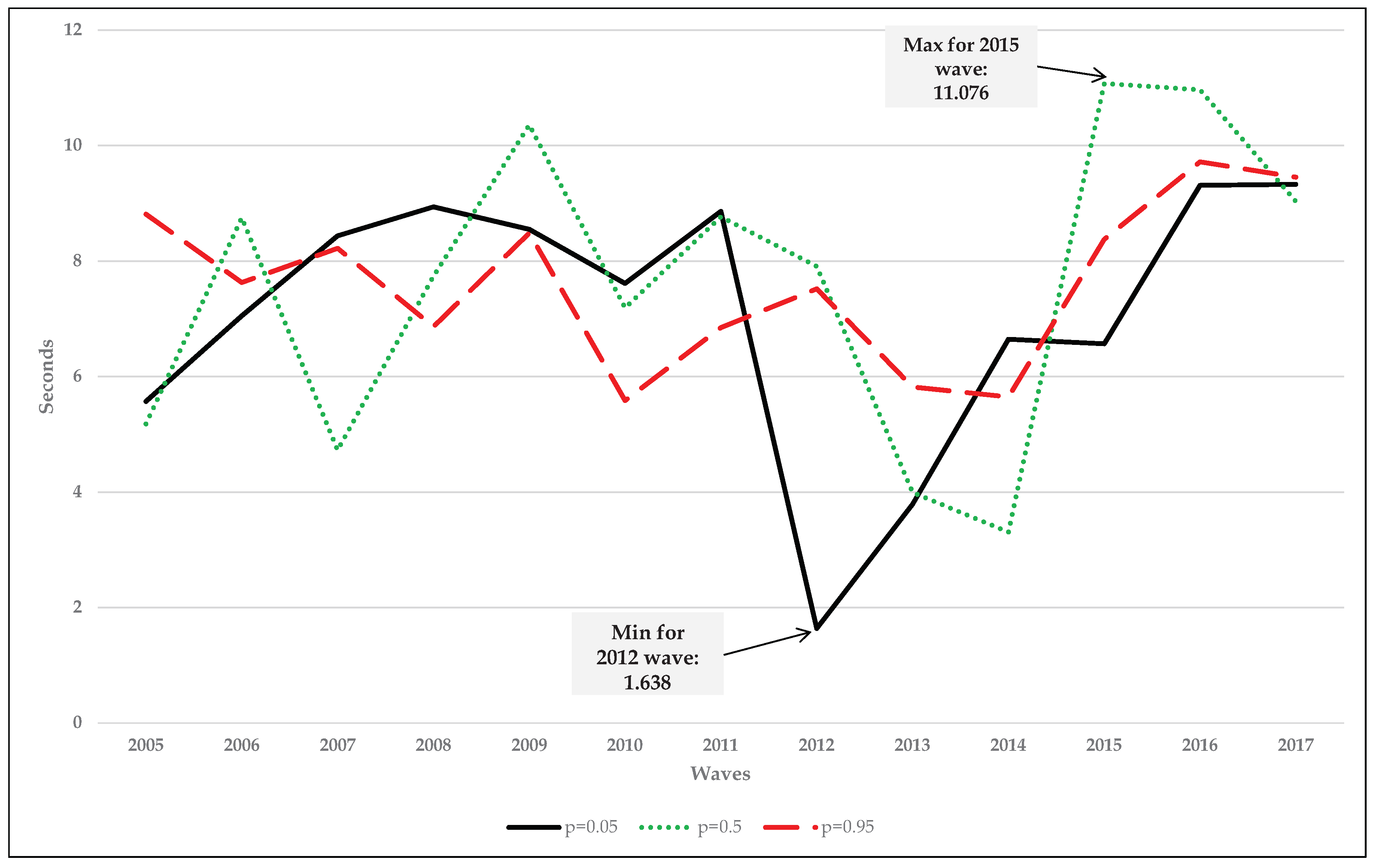
| 2012 | 358,046 | 354,395 | 339,223 | 3.975 | 3.935 | 3.766 | 99.39 | 98.38 | 94.17 | 1.638 | 7.910 | 7.519 | 5.332 | Negligible |
| 2013 | 158,486 | 92,024 | 52,502 | 1.732 | 1.005 | 0.574 | 43.59 | 25.31 | 14.44 | 3.791 | 3.994 | 5.819 | 4.939 | Negligible |
| 2014 | 186,109 | 112,455 | 66,322 | 2.005 | 1.212 | 0.715 | 50.48 | 30.50 | 17.99 | 6.646 | 3.307 | 5.648 | 4.666 | Negligible |
| 2015 | 371,174 | 369,381 | 364,563 | 3.969 | 3.950 | 3.898 | 99.20 | 98.72 | 97.43 | 6.568 | 11.076 | 8.377 | 4.588 | Negligible |
| 2016 | 376,017 | 372,166 | 309,241 | 3.973 | 3.932 | 3.267 | 99.22 | 98.20 | 81.60 | 9.313 | 10.967 | 9.719 | 1.497 | Negligible |
| 2017 | 378,463 | 352,488 | 278,254 | 3.954 | 3.682 | 2.907 | 99.13 | 92.32 | 72.88 | 9.329 | 9.032 | 9.453 | 1.012 | Negligible |
| CSWL | |||||||||||||
| Type of Pension | 2005 | 2006 | 2007 | 2008 | 2009 | 2010 | 2011 | 2012 | 2013 | 2014 | 2015 | 2016 | 2017 |
| Perm. Disability M | 0.000000 | 0.000000 | 0.261722 | 0.000000 | 0.000000 | 0.000000 | 0.000000 | 0.000000 | 0.000000 | 0.000000 | 0.000000 | 0.000000 | 0.000000 |
| Perm. Disability F | 0.000000 | 0.000000 | 0.022240 | 0.000000 | 0.000000 | 0.000000 | 0.000000 | 0.000000 | 0.187779 | 0.042312 | 0.000000 | 0.000000 | 0.000021 |
| Retirement M | 0.000000 | 0.000004 | 0.000001 | 0.000000 | 0.000000 | 0.000000 | 0.000000 | 0.005268 | 0.140715 | 0.013956 | 0.000743 | 0.001314 | 0.002751 |
| Retirement F | 0.000000 | 0.000000 | 0.000000 | 0.000000 | 0.000000 | 0.000000 | 0.000000 | 0.001217 | 0.000120 | 0.000052 | 0.000011 | 0.000065 | 0.013070 |
| Widower’s M | 0.000000 | 0.000000 | 0.000000 | 0.000000 | 0.000000 | 0.000000 | 0.000000 | 0.000000 | 0.000000 | 0.000000 | 0.000000 | 0.000000 | 0.000000 |
| Widow’s F | 0.000000 | 0.000000 | 0.000000 | 0.000000 | 0.000000 | 0.000000 | 0.000000 | 0.000014 | 0.000006 | 0.000451 | 0.009670 | 0.008186 | 0.208145 |
| Orphan’s M | 0.000000 | 0.005082 | 0.202030 | 0.261090 | 0.591337 | 0.462422 | 0.837630 | 0.944315 | 0.593409 | 0.370949 | 0.849506 | 0.000039 | 0.112380 |
| Orphan’s F | 0.000000 | 0.118497 | 0.164789 | 0.141561 | 0.393848 | 0.561802 | 0.296694 | 0.117598 | 0.106684 | 0.285731 | 0.000101 | 0.000000 | 0.070073 |
| Family Responsib. M | 0.002755 | 0.111863 | 0.115631 | 0.396466 | 0.061782 | 0.428490 | 0.208140 | 0.323662 | 0.463862 | 0.327626 | 0.834403 | 0.830553 | 0.915809 |
| Family Responsib. F | 0.003573 | 0.249222 | 0.154051 | 0.021609 | 0.689061 | 0.841654 | 0.960454 | 0.333362 | 0.156821 | 0.659514 | 0.886466 | 0.344878 | 0.758455 |
| Total Pensions | 0.000000 | 0.000000 | 0.000000 | 0.000000 | 0.000000 | 0.000000 | 0.000000 | 0.000000 | 0.000000 | 0.000000 | 0.000000 | 0.000000 | 0.000000 |
| Subsample with p-value = | |||||||||||||
| Type of Pension | 2005 | 2006 | 2007 | 2008 | 2009 | 2010 | 2011 | 2012 | 2013 | 2014 | 2015 | 2016 | 2017 |
| Perm. Disability M | 0.999062 | 0.997165 | 1.000000 | 1.000000 | 0.999995 | 0.999884 | 1.000000 | 1.000000 | 0.050022 | 0.050023 | 0.999079 | 0.999962 | 1.000000 |
| Perm. Disability F | 0.050167 | 1.000000 | 0.999935 | 1.000000 | 0.999449 | 0.999896 | 0.998295 | 0.986718 | 1.000000 | 0.95254 | 0.998444 | 0.999978 | 0.990695 |
| Retirement M | 1.000000 | 0.992407 | 0.999452 | 0.674773 | 0.105610 | 0.113748 | 0.050031 | 0.136429 | 0.999905 | 0.999937 | 0.433788 | 0.050327 | 0.050202 |
| Retirement F | 0.999948 | 0.999994 | 1.000000 | 0.734123 | 0.050021 | 0.050184 | 0.237496 | 0.536713 | 0.999268 | 0.999864 | 0.050727 | 0.068528 | 0.495790 |
| Widower’s M | 1.000000 | 0.050289 | 0.050099 | 0.050117 | 0.094137 | 0.289216 | 0.361538 | 0.205785 | 1.000000 | 1.000000 | 0.90782 | 0.903889 | 0.926686 |
| Widow’s F | 1.000000 | 1.000000 | 1.000000 | 1.000000 | 1.000000 | 1.000000 | 1.000000 | 0.997186 | 1.000000 | 1.000000 | 0.886394 | 0.946287 | 0.999344 |
| Orphan’s M | 1.000000 | 0.973781 | 0.974972 | 0.996229 | 0.997206 | 0.999660 | 0.999868 | 0.999343 | 1.000000 | 1.000000 | 0.998689 | 0.982116 | 0.968999 |
| Orphan’s F | 1.000000 | 0.994200 | 0.992617 | 0.999344 | 0.996990 | 1.000000 | 0.999810 | 0.999604 | 1.000000 | 1.000000 | 1.000000 | 1.000000 | 0.999870 |
| Family Responsib. M | 0.485665 | 0.452965 | 0.870183 | 0.960915 | 0.834992 | 0.984285 | 0.739576 | 0.894736 | 1.000000 | 0.999996 | 0.984555 | 0.992232 | 0.987172 |
| Family Responsib. F | 0.592029 | 0.958494 | 0.915957 | 0.995480 | 0.997873 | 0.997951 | 0.994521 | 0.839826 | 0.999999 | 0.999998 | 0.999575 | 0.999999 | 0.999967 |
| Total Pensions | 1.000000 | 1.000000 | 1.000000 | 1.000000 | 0.999999 | 1.000000 | 1.000000 | 1.000000 | 1.000000 | 1.000000 | 1.000000 | 1.000000 | 1.000000 |
| Subsample with p-value = | |||||||||||||
| Type of Pension | 2005 | 2006 | 2007 | 2008 | 2009 | 2010 | 2011 | 2012 | 2013 | 2014 | 2015 | 2016 | 2017 |
| Perm. Disability M | 0.999824 | 0.998681 | 1.000000 | 1.000000 | 1.000000 | 0.999995 | 1.000000 | 1.000000 | 0.500135 | 0.500169 | 0.99989 | 1.000000 | 1.000000 |
| Perm. Disability F | 0.500237 | 1.000000 | 1.000000 | 1.000000 | 0.999988 | 0.999996 | 0.999946 | 0.999053 | 1.000000 | 0.999968 | 0.999604 | 0.999998 | 1.000000 |
| Retirement M | 1.000000 | 0.999888 | 1.000000 | 1.000000 | 0.993192 | 0.500103 | 0.500086 | 0.742335 | 0.999991 | 0.999987 | 0.834558 | 0.500022 | 0.500002 |
| Retirement F | 0.999996 | 1.000000 | 1.000000 | 1.000000 | 0.974744 | 0.831733 | 0.999998 | 0.998129 | 0.999696 | 0.999979 | 0.500139 | 0.888871 | 0.999492 |
| Widower’s M | 1.000000 | 0.500484 | 0.500491 | 0.500446 | 0.500167 | 0.704613 | 0.973377 | 0.500940 | 1.000000 | 1.000000 | 0.974067 | 0.994449 | 1.000000 |
| Widow’s F | 1.000000 | 1.000000 | 1.000000 | 1.000000 | 1.000000 | 1.000000 | 1.000000 | 1.000000 | 1.000000 | 1.000000 | 0.999922 | 1.000000 | 1.000000 |
| Orphan’s M | 1.000000 | 0.993038 | 0.990978 | 0.999867 | 0.999881 | 0.999983 | 1.000000 | 0.999930 | 1.000000 | 1.000000 | 0.999604 | 0.99941 | 1.000000 |
| Orphan’s F | 1.000000 | 0.998723 | 0.998609 | 0.999976 | 0.998971 | 1.000000 | 0.999987 | 0.999933 | 1.000000 | 1.000000 | 1.000000 | 1.000000 | 1.000000 |
| Family Responsib. M | 0.596180 | 0.516585 | 0.926654 | 0.981715 | 0.865071 | 0.991481 | 0.815663 | 0.908726 | 1.000000 | 0.999994 | 0.986995 | 0.995072 | 0.996236 |
| Family Responsib. F | 0.730443 | 0.983661 | 0.965339 | 0.998284 | 0.999231 | 0.999351 | 0.997099 | 0.879598 | 1.000000 | 1.000000 | 0.999852 | 1.000000 | 1.000000 |
| Total Pensions | 1.000000 | 1.000000 | 1.000000 | 1.000000 | 1.000000 | 1.000000 | 1.000000 | 1.000000 | 1.000000 | 1.000000 | 1.000000 | 1.000000 | 1.000000 |
| Subsample with p-value = | |||||||||||||
| Type of Pension | 2005 | 2006 | 2007 | 2008 | 2009 | 2010 | 2011 | 2012 | 2013 | 2014 | 2015 | 2016 | 2017 |
| Perm. Disability M | 1.000000 | 1.000000 | 1.000000 | 1.000000 | 1.000000 | 1.000000 | 1.000000 | 1.000000 | 0.975219 | 0.950021 | 1.000000 | 1.000000 | 1.000000 |
| Perm. Disability F | 1.000000 | 1.000000 | 1.000000 | 1.000000 | 1.000000 | 1.000000 | 1.000000 | 1.000000 | 1.000000 | 1.000000 | 0.999985 | 1.000000 | 1.000000 |
| Retirement M | 1.000000 | 1.000000 | 1.000000 | 1.000000 | 1.000000 | 0.950005 | 0.999992 | 0.996452 | 0.999993 | 0.999999 | 0.950024 | 0.950063 | 0.950000 |
| Retirement F | 1.000000 | 1.000000 | 1.000000 | 0.999996 | 1.000000 | 0.999897 | 0.999986 | 0.999985 | 0.999986 | 0.999988 | 0.962697 | 1.000000 | 0.999905 |
| Widower’s M | 1.000000 | 1.000000 | 0.950055 | 0.950193 | 0.999535 | 0.999988 | 1.000000 | 0.999689 | 1.000000 | 1.000000 | 0.999129 | 1.000000 | 1.000000 |
| Widow’s F | 1.000000 | 1.000000 | 1.000000 | 1.000000 | 1.000000 | 1.000000 | 1.000000 | 1.000000 | 1.000000 | 1.000000 | 1.000000 | 1.000000 | 1.000000 |
| Orphan’s M | 1.000000 | 1.000000 | 0.995183 | 0.999997 | 1.000000 | 1.000000 | 1.000000 | 1.000000 | 1.000000 | 1.000000 | 0.999970 | 1.000000 | 1.000000 |
| Orphan’s F | 1.000000 | 1.000000 | 0.999779 | 1.000000 | 0.999919 | 1.000000 | 1.000000 | 1.000000 | 1.000000 | 1.000000 | 1.000000 | 1.000000 | 1.000000 |
| Family Responsib. M | 0.950041 | 0.950010 | 0.962938 | 0.992756 | 0.950023 | 0.999119 | 0.950023 | 0.950006 | 0.999987 | 0.998926 | 0.989983 | 0.999760 | 0.999937 |
| Family Responsib. F | 0.987717 | 0.999995 | 0.984731 | 0.999267 | 0.99988 | 0.999992 | 0.999793 | 0.950267 | 0.999999 | 1.000000 | 0.999985 | 1.000000 | 1.000000 |
| Total Pensions | 1.000000 | 1.000000 | 1.000000 | 1.000000 | 1.000000 | 1.000000 | 1.000000 | 1.000000 | 1.000000 | 1.000000 | 1.000000 | 1.000000 | 1.000000 |
© 2020 by the authors. Licensee MDPI, Basel, Switzerland. This article is an open access article distributed under the terms and conditions of the Creative Commons Attribution (CC BY) license (http://creativecommons.org/licenses/by/4.0/).
Share and Cite
Núñez-Antón, V.; Pérez-Salamero González, J.M.; Regúlez-Castillo, M.; Vidal-Meliá, C. Improving the Representativeness of a Simple Random Sample: An Optimization Model and Its Application to the Continuous Sample of Working Lives. Mathematics 2020, 8, 1225. https://doi.org/10.3390/math8081225
Núñez-Antón V, Pérez-Salamero González JM, Regúlez-Castillo M, Vidal-Meliá C. Improving the Representativeness of a Simple Random Sample: An Optimization Model and Its Application to the Continuous Sample of Working Lives. Mathematics. 2020; 8(8):1225. https://doi.org/10.3390/math8081225
Chicago/Turabian StyleNúñez-Antón, Vicente, Juan Manuel Pérez-Salamero González, Marta Regúlez-Castillo, and Carlos Vidal-Meliá. 2020. "Improving the Representativeness of a Simple Random Sample: An Optimization Model and Its Application to the Continuous Sample of Working Lives" Mathematics 8, no. 8: 1225. https://doi.org/10.3390/math8081225
APA StyleNúñez-Antón, V., Pérez-Salamero González, J. M., Regúlez-Castillo, M., & Vidal-Meliá, C. (2020). Improving the Representativeness of a Simple Random Sample: An Optimization Model and Its Application to the Continuous Sample of Working Lives. Mathematics, 8(8), 1225. https://doi.org/10.3390/math8081225