4.1. Mechanisms Affecting Unfrozen Water Content
The relatively high clay content in the soil, close to 50% (
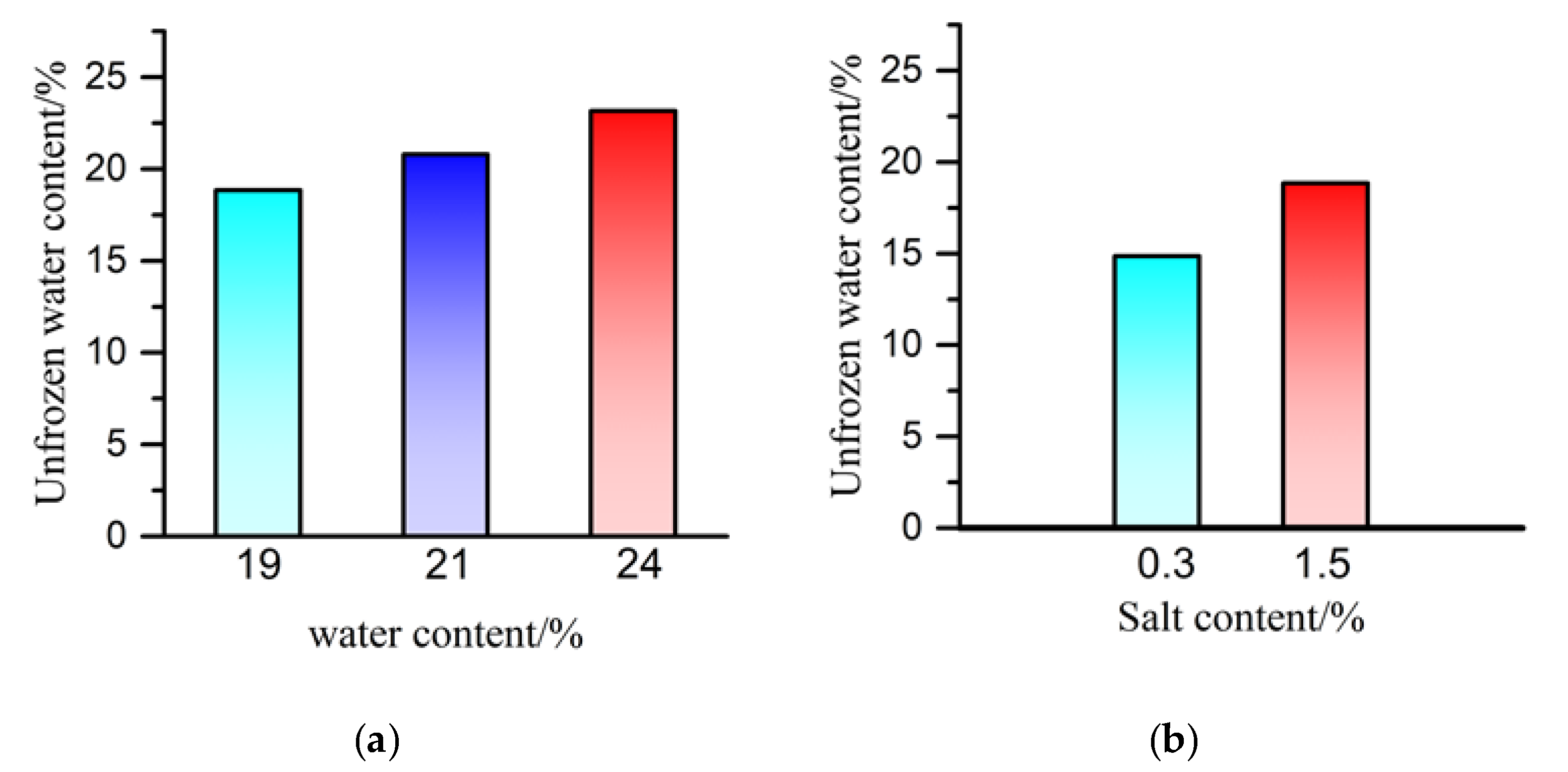
Figure 1), showed that the specific surface area of the soil was relatively large, and the soil particles had a strong adsorption capacity for the water molecules. The water molecules were gathered around the soil particles through the adsorption capacity of the soil particles, thus forming a water film. The higher the initial water content was, the thicker the water film. At the same temperature, this phenomenon led to higher initial water content, a higher UW, and the same change trend for UW and water content, as shown in
Figure 5a. In
Figure 5a, the green bar, blue bar, and red bar represent the UW of the soil samples with water content of 19%, 21%, and 24%.
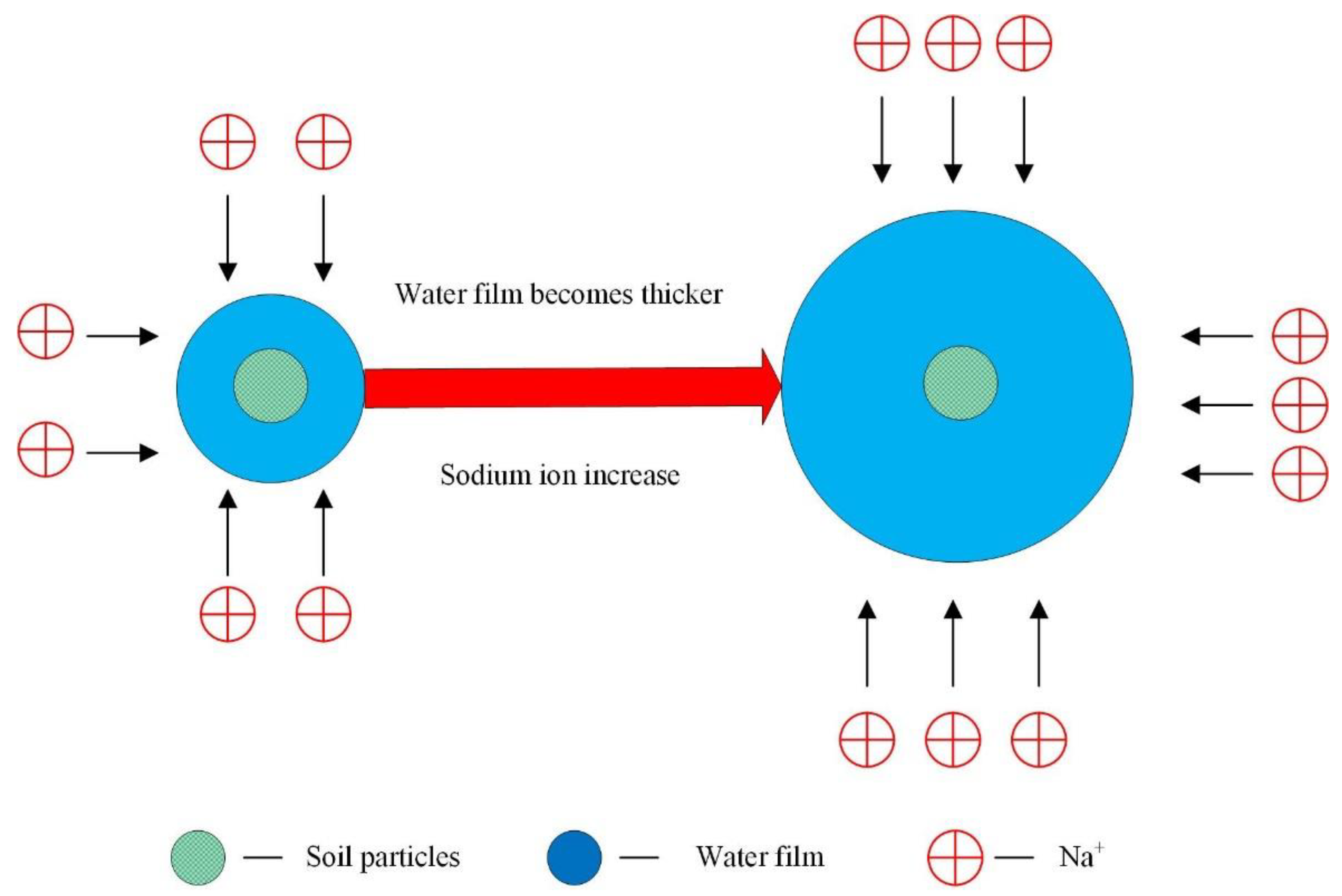
The soil mainly contained sodium bicarbonate, so the content of sodium ions was relatively high. The clay minerals in the soil contained some highly hydrophilic minerals, such as illite and illite/smectite mixed layer minerals (
Figure 2). When the highly hydrophilic minerals interacted with the sodium ions in the sodium salt, a large amount of thin film water (weakly bound water) gathered around the soil particles. With an increase in sodium ions, the water film gradually thickened (
Figure 6), showing the UW to increase as with the water film thickened. Therefore, at the same temperature, the salt content increased, which indirectly inhibited the freezing of the soil, resulting in an increased UW. The UW and the salt content also maintained the same change trend, as shown in
Figure 5b. In the
Figure 5b, the green bar and red bar represent the UW of the soil sample with salt content of 0.3% and 1.5%.
When the outside temperature is less than 0 °C and continues to decrease, unfrozen water appears in the soil, and as a whole, the UW decreases as the temperature decreases [
44]. Therefore, it is self-evident that temperature is the main factor affecting changes in UW.
4.3. Compare and Select the Model
After determining the weights of the influencing factors, the AHP-entropy-ANFIS model was established in combination with ANFIS. This model was compared with the ANFIS model, the SVM model and the AHP-entropy-SVM model, and the model with the strongest predictive ability was selected to predict the UW. In this paper, temperature, salt content, and initial water content were input into the models, and the UW of saline soil was the output factor of the models. The training and testing of the models were realized on the MATLAB software platform. In the ANFIS prediction model, according to actual needs, a total of 27 different “If-Then” rules were formulated, and the “trimf”-type function, with an improved training effect, was selected as the membership function [
31,
43]. In the SVM prediction model, the “radial basis” function is an important part of the model. It is the main method for the model to process data. The SVM model applies the grid search method, and combines the penalty parameter and radial basis kernel factor to train the model [
36].
In addition, in the process of training and testing, a five-fold cross-validation method was used to avoid the problem of overfitting the model. Through this five-fold cross-validation, the coefficient of determination, the mean squared error, and the
p-value of each model was obtained, as shown in
Table 7.
The data in
Table 7 were then analyzed. In the process of training, the mean R
2 values of the four models (AHP-entropy-ANFIS, ANFIS, SVM, and AHP-entropy-SVM models) were all greater than 0.8, and the mean R
2 of the AHP-entropy-ANFIS model was the highest, reaching 0.9935. The mean MSEs of the four models were 0.14, 0.19, 2.99, and 2.78, respectively. Clearly AHP-entropy-ANFIS (0.14) was the smallest. For the stability of the model, the order from high to low was as follows: the AHP-entropy-ANFIS model, the ANFIS model, the AHP-entropy-SVM model, and the SVM model.
In the process of testing, the four models were compared. The mean R2 the of the AHP-entropy-ANFIS model was the largest, at 0.9692. The mean MSE of this model was 0.86, making it the smallest. Compared to the training process, the stability of the AHP-entropy-ANFIS model, the ANFIS model, the AHP-entropy-SVM model and the SVM model were slightly reduced, but the AHP-entropy-ANFIS model remained the most stable. The AHP-entropy-ANFIS model thus performed the best. In addition, in the process of training and testing, the p-values of the models were less than 0.05.
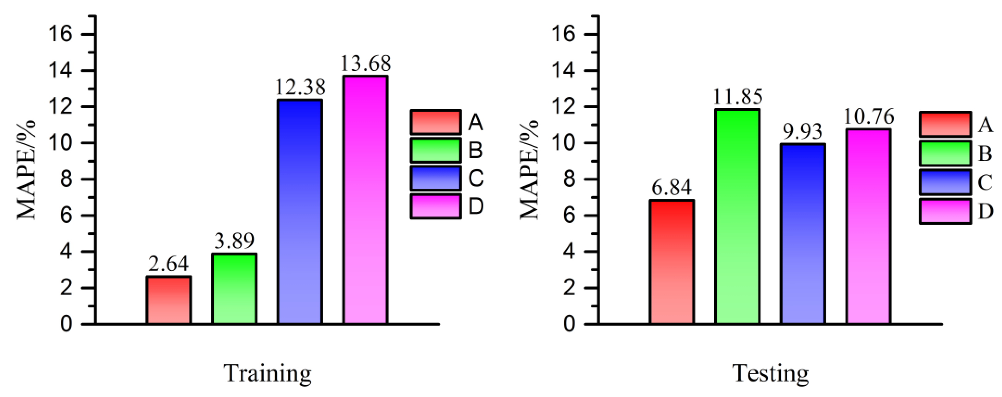
Figure 7 describes the mean absolute percent errors (MAPEs) of the different models. Among them, legend A is the AHP-entropy-ANFIS model, legend B is the ANFIS model, legend C is the SVM model, and legend D is the AHP-entropy-SVM model. It can be seen from
Figure 7 that in both the training process and the testing process, the MAPE of the AHP-entropy-ANFIS model was less than that of the other three models, and the MAPE of the AHP-entropy-ANFIS model was less than 10. In the training process, the MAPE of the AHP-entropy-ANFIS model was about 1/1.5 that of the ANFIS model, and the MAPE of the AHP-entropy-ANFIS model was about 1/5 that of the AHP-entropy-SVM model. In the testing process, the MAPE of the AHP-entropy-ANFIS model was about 1/1.5 that of the SVM model, and about 1/2 that of the ANFIS model.
Figure 8 describes the mean absolute errors (MAEs) of the different models: legend A is the AHP-entropy-ANFIS model, legend B is the ANFIS model, legend C is the SVM model, and legend D is the AHP-entropy-SVM model. As shown in
Figure 8, compared with the other three models, the MAE of the AHP-entropy-ANFIS model was the smallest, at less than 1. During the training process, the MAE of the AHP-entropy-ANFIS model was about 1/1.6 that of the ANFIS model, and about 1/6 that of the AHP-entropy-SVM model. During the testing process, the MAE of the AHP-entropy-ANFIS model was about 1/1.3 that of the SVM model, and about 1/1.6 that of the ANFIS model.
In addition, the predicted values and test values of the different models were compared, and the models’ ability to predict the UW of saline soil was judged by the conclusions obtained.
Figure 9 describes the relationship between the data output by the different models during the training process and the real (experimental) data. As shown in
Figure 9, compared with the ANFIS model, the prediction result of the AHP-entropy-ANFIS model was closest to the real experimental value. The changes in the blue curve and red curve are very similar; the difference between the two curves is very small, and the two curves basically coincide. The performance of the SVM and AHP-entropy-SVM models was slightly worse, as the blue and red curves are not completely coincident. Although the changes in the two curves are similar, they present some differences. This result reveals that, compared with the other three models, the AHP-entropy-ANFIS model provided a stronger fitting capability and better performance during the training process.
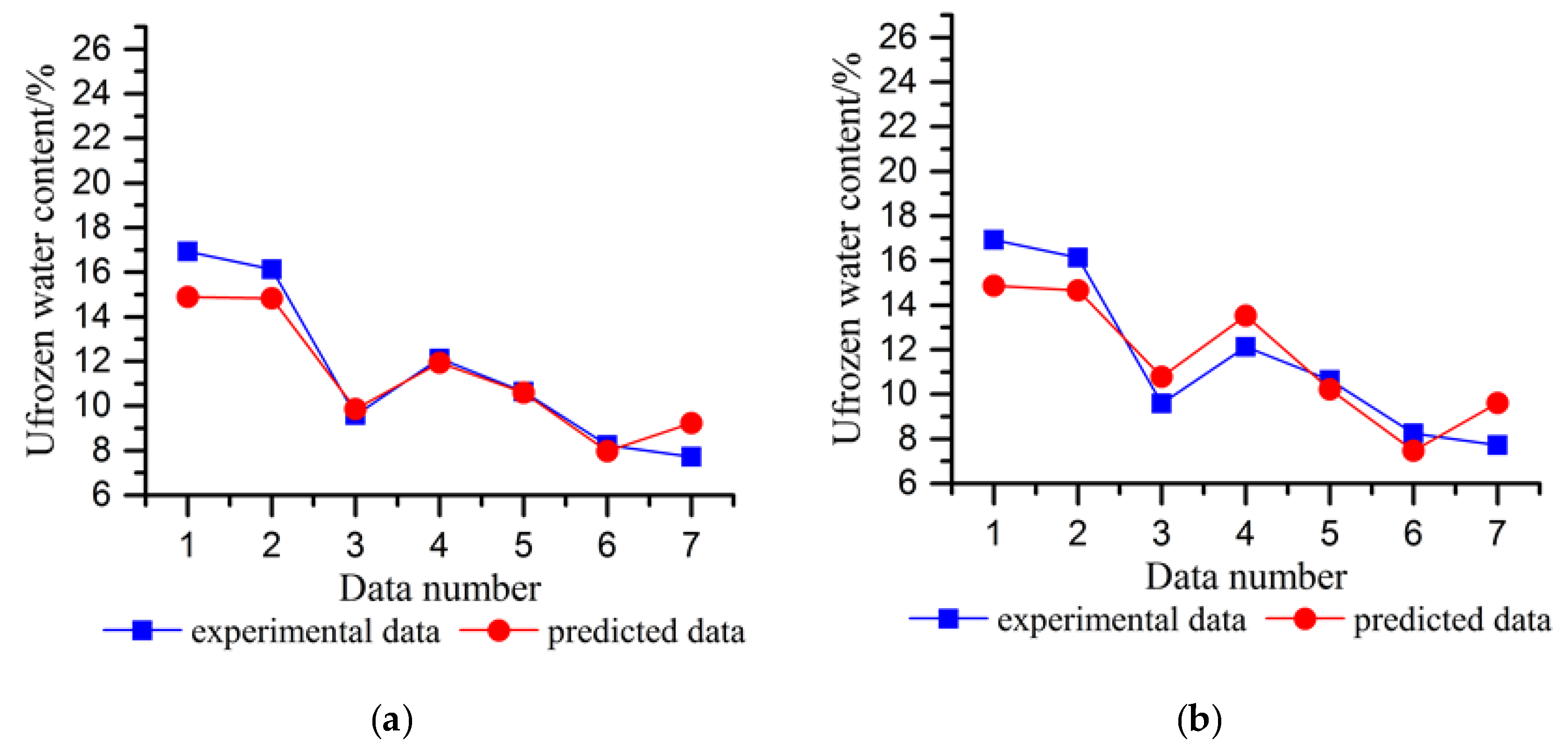
Figure 10 describes the relationship between the data output by the different models during the testing process and the real data. As described in
Figure 10a, the variations in the blue and red curves are similar, and there is only a small difference. In the two curves, the curve corresponding to data points 2 to 6 basically coincides. Thus, the error of the AHP-entropy-ANFIS model is smaller. In
Figure 10b–d, the data point corresponding to the red curve becomes larger or smaller, resulting in a large difference between the red and blue curves. This shows that during the test process, compared with the AHP-entropy-ANFIS model, the other three models provided a weaker fitting ability and poorer performance.
Xu [
45], Anderson and Tice [
46] studied the unfrozen water content. They built empirical models on the basis of experiments to predict the unfrozen water content. The unfrozen water content is obtained through empirical formulas, but only the unfrozen water content corresponding to the freezing temperature can be obtained, and the complete unfrozen water content change characteristic curve cannot be obtained. So, the models established in this paper can better predict the unfrozen water content.
In short, through the comparative analysis of the statistical factors, the predicted values, and the experimental values of the different models, it was found that, compared with the ANFIS, SVM and AHP-entropy-SVM models, the AHP-entropy-ANFIS model can produce smaller prediction errors and have a stronger fitting ability. Therefore, the AHP-entropy-ANFIS model offers better prediction capability. Consequently, the AHP-entropy-ANFIS model is the best choice for predicting the UW of saline soil in Zhenlai.


 and
and 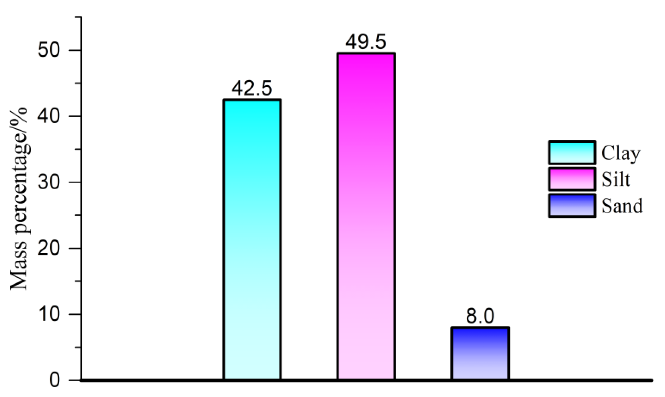


