Using a Fuzzy Inference System to Obtain Technological Tables for Electrical Discharge Machining Processes

Abstract

Technological tables are very important in electrical discharge machining to determine optimal operating conditions for process variables, such as material removal rate or electrode wear. Their determination is of great industrial importance and their experimental determination is very important because they allow the most appropriate operating conditions to be selected beforehand. These technological tables are usually employed for electrical discharge machining of steel, but their number is significantly less in the case of other materials. In this present research study, a methodology based on using a fuzzy inference system to obtain these technological tables is shown with the aim of being able to select the most appropriate manufacturing conditions in advance. In addition, a study of the results obtained using a fuzzy inference system for modeling the behavior of electrical discharge machining parameters is shown. These results are compared to those obtained from response surface methodology. Furthermore, it is demonstrated that the fuzzy system can provide a high degree of precision and, therefore, it can be used to determine the influence of these machining parameters on technological variables, such as roughness, electrode wear, or material removal rate, more efficiently than other techniques.

1. Introduction

Electrical discharge machining (EDM) is a manufacturing process which is typically classified as a non-traditional manufacturing process. EDM has several advantages over traditional manufacturing processes such as turning or milling, because there is no direct contact between the part and the tool, and the hardness of the so-processed materials does not affect the result. In the field of EDM, technological tables are of great interest since, by using them, it is possible to determine in advance the optimal machining conditions for a certain strategy that either maximizes material removal or reduces electrode wear, among other objectives. These technological tables are usually employed for electrical discharge machining of steel, but their number is significantly less in the case of other materials. In the research study of Torres et al. [1], technological tables were obtained for the case of TiB₂, which is a low-machinability material, by using response surface methodology (RSM) that fitted a second-order polynomial regression model along with nonlinear programming. However, when regression models are not adequate to predict the behavior of response variables, because the values of the coefficients of determination are low, it is necessary to use other alternative methodologies. Therefore, in this present study, a methodology is proposed to obtain the technological tables using a Sugeno type fuzzy inference system (FIS). As shown, the results obtained with this FIS significantly improve those obtained using response surface methodology and, therefore, the results obtained are more reliable than those obtained by RSM. In the research study of Torres et al. [2], a new energy density model was proposed and a 4³ factorial design was employed for modeling the behavior of the arithmetical mean roughness (Ra), the electrode wear (EW), and the material removal rate (MRR) in the EDM machining of an Inconel^® 600 alloy using Cu–C electrodes (Inconel is a registered trademark of Special Metals Family of Companies). However, in this study, the technological tables for this alloy were not developed. Furthermore, as shown in this study [2], the regression models obtained using RSM were able to adequately predict Ra and MRR values with R-squared values greater than 0.95; however, in the case of EW, response surface methodology was not able to adequately predict the EW behavior. Therefore, to fill these gaps, a Takagi–Sugeno [3,4] fuzzy inference system (FIS) is proposed in this present study to model the behavior of Ra, MRR, and EW and to obtain the technological tables for this Inconel^® 600 alloy, within the range of the considered variation levels of the parameters under study. In addition, a comparative study is performed between the results provided by RSM and the results provided by the FIS system. In [5] a methodology was developed to obtain the values of technological tables for the case of B₄C, SiSiC and WC-Co conductive ceramic materials. However, as in the technological tables developed in [1], when regression models are not adequate to predict the behaviour of response variables, it is necessary to use other alternative methodologies. As shown below, the FIS can predict the output values more efficiently than by using regression. Data shown in

Table 1. Design factors and levels. These values were taken from Reference [2] Torres Salcedo, A.; Puertas Arbizu I.; Luis Pérez, C. J. Analytical Modeling of Energy Density and Optimization of the EDM Machining Parameters of Inconel 600. Metals 2017, 7, 166. (Open access article distributed under the terms and conditions of the Creative Commons Attribution (CC BY) license: http://creativecommons.org/licenses/by/4.0/).

Design Factors	Levels and Values
	Positive Polarity				Negative Polarity
	1	2	3	4	1	2	3	4
Current intensity $\left(\mathrm{A}\right)$	2	4	6	8	2	4	6	8
Pulse time $\left(\mathsf{\mu }\mathrm{s}\right)$	25	50	75	100	25	50	75	100
Duty cycle $(\%)$	0.3	0.4	0.5	0.6	0.3	0.4	0.5	0.6

and

Table 2. Mean values of arithmetical mean roughness (Ra), material removal rate (MRR), and electrode wear (EW), obtained with positive and negative polarity. These values were taken from Reference [2] Torres Salcedo, A.; Puertas Arbizu I.; Luis Pérez, C. J. Analytical Modeling of Energy Density and Optimization of the EDM Machining Parameters of Inconel 600. Metals 2017, 7, 166. (Open access article distributed under the terms and conditions of the Creative Commons Attribution (CC BY) license: http://creativecommons.org/licenses/by/4.0/). (See Reference [2] or Appendix A for all data).

	Positive Polarity (+)			Negative Polarity (−)
E	Ra (µm)	MRR (mm3/min)	EW (%)	E	Ra (µm)	MRR (mm3/min)	EW (%)
1	1.39	0.1778	35.81	1	1.57	0.4961	96.67
2	3.34	3.0897	10.66	2	3.59	4.7944	28.23
63	6.33	8.4132	1.30	63	7.52	23.2371	171.94
64	7.08	15.3894	0.37	64	7.83	30.4894	17.49

that were taken from the above-mentioned study [2] are used in this present work in order to analyze a case study and to develop a fuzzy inference system for modeling the behavior of these technological variables (Ra, EW, and MRR), as well as show the application of the proposed methodology in order to obtain the technological tables. These technological tables are widely used for steel, while their number is significantly less in the case of other materials. In any case, it is considered that the proposed methodology could be generally applied to any other material and for other manufacturing processes. Hence, it is considered that the present methodology for obtaining the technological tables may be of interest in the event that the input variables can be continuously varied and, thus, in this way, it could be possible to select the most appropriate operating conditions in advance.

2. State of the Art

Over the past few years, the number of applications of fuzzy systems increased significantly [6]. Takagi–Sugeno [3,4] and Mamdani [7,8] fuzzy inference systems are commonly used, and there exist a large number of research studies in different scientific fields, dealing with control, pattern recognition, modeling, etc. Among the studies that can be found in the literature, it is worth mentioning the study of Mouralova et al. [9] which proposed a Mamdani FIS, based on 18 rules provided by an expert in the field, for modeling the cutting speed in wire electrical discharge machining (WEDM) from five inputs (gap voltage, pulse on time, pulse off time, discharge current, and wire feed). These authors employed a maximum of results for aggregation and the centroid in order to de-fuzzify the aggregated output. Among the conclusions, these authors found that the FIS may be employed in order to determine the optimum machine parameters to maximize the cutting speed for the WEDM of Creusabro steel [9]. In another study, Aamir et al. [10] employed a Mamdani FIS to predict surface roughness and hole size as a function of feed rate and cutting speed in multi-hole drilling. These authors calculated the outputs based on the centroid method. They found that the FIS was able to predict hole quality at different levels of process parameters [10]. On the other hand, Alarifi et al. [11] employed genetic algorithms and particle swarm optimization to determine the parameters of an adaptive neuro-fuzzy inference system (ANFIS) model to predict the thermo-physical properties of Al₂O₃–multi-walled carbon nanotube (MWCNT)/thermal oil hybrid nanofluid. In order to evaluate and compare the performance of the models analyzed, root-mean-square error (RMSE) and the R-squared coefficient (R²) were employed. These authors found that the models were able to appropriately predict the thermo-physical properties [11]. In the research study of Wang et al. [12], a fuzzy multicriteria decision-making model (MCDM) for raw material supplier selection in the plastic industry was employed. Likewise, in the research study of Kang et al. [13], a heating temperature estimation method using an ANFIS algorithm was proposed for diagnosis and assessment of fire-damaged concrete structures. These authors employed as input variables ultrasonic pulse velocity, reflectance of the concrete surface, and design compressive strength of the concrete. Moreover, these authors estimated the heating temperatures of the specimens using the proposed ANFIS algorithm. They found that their model estimated the heating temperatures of the specimens with a high degree of accuracy [13]. On the other hand, Tayyab et al. [14] applied fuzzy theory to consider uncertainty in demand information in a multi-stage lean manufacturing system. These authors employed the centroid to de-fuzzify the objective function. Other studies such as that of Faisal et al. [15] used particle swarm optimization (PSO) and biogeography-based optimization (BBO) algorithms for a multiple-objective optimization of the MRR and Ra for the EDM process, and they validated their models with experimental results. Lin et al. [16] applied a fuzzy collaborative intelligence approach for fall detection in four existing smart technology applications, while Cavallaro employed a Takagi–Sugeno FIS to assess the sustainability of biomass of production [17].

Regarding fuzzy modeling for industrial applications, there exist several studies which were applied to different industrial sectors. Among these research studies, it is worth mentioning the application of soft computing techniques for both detection and classification of defects [18,19], fault diagnosis of rolling bearing in industrial robots [20], airport classification [21], control of piezoelectric actuators [22], monitoring of fuel system of an industrial gas turbine [23], control of brushless direct current (DC) motors [24], and fault detection in wind turbines [25]. In addition, fuzzy systems are able to handle uncertainties in an efficient way, as shown in Reference [26], where a Takagi–Sugeno–Kang (TSK) type-2 fuzzy neural network was proposed for system modeling and noise cancellation, or in Reference [27], where a design methodology based on interval type-2 TSK fuzzy logic controllers for modular and reconfigurable robots manipulators with uncertain dynamic parameters was shown, among many others [28,29].

Some other studies such as that of Shabgard et al. [30] employed a Mamdani inference system to predict material removal rate, electrode wear, and surface roughness in the EDM and ultrasonic-assisted EDM (US/EDM) processes of tungsten carbide. An analysis of the particle swarm optimization (PSO) implementation in designing parameters of manufacturing processes, as well as a benchmark with other optimization techniques can be found in the review study of Sibalija [31]. EDM process variables were modeled by using artificial neural networks (ANNs) and ANFIS, as shown in studies such as that of Rahul et al. [32], where the authors employed a Taguchy design of experiments, as well as the concept of satisfaction function, to improve machining performances responses in EDM of Inconel 718. Babu et al. [33] employed a Taguchy design of experiments and an ANN in order to determine optimal parameters in the wire electrical discharge machining (WEDM) of Inconel 750. Likewise, Al-Ghamdi et al. employed an adaptive neuro-fuzzy inference system (ANFIS) and polynomial modeling approaches to model the material removal rate in EDM of a Ti–6Al–4V alloy [34]. These authors employed five ANFIS models and a first-order Sugeno, along with a back-propagation neural network training algorithm. Among the results, these authors found that ANFIS models perform more efficiently than convectional polynomial models [34]. Devarasiddappa et al. [35] employed an artificial neural network (ANN) to predict surface roughness in the wire-cut electrical discharge machining (WEDM) of Inconel 825. These authors found that this methodology is effective for modeling surface roughness in this Inconel alloy [35]. Maher et al. [36] employed an adaptive neuro-fuzzy inference system (ANFIS) to predict cutting speed, surface roughness, and heat-affected zone in WEDM. Another example is the study of Joshi et al. [37] which investigated the management and quantification of surface roughness and MRR of Inconel 800 HT when machined with a copper electrode on EDM, whereas Torres et al. [38] studied an Inconel^® 718 alloy during electrical discharge machining.

From previous studies, it is possible to see that EDM is commonly used for manufacturing materials such as tungsten carbide [39], titanium diboride [1], and Inconel^® alloys [2], boron carbide and silicon carbide [5], among many others. In this present research study, the main aim is to use a FIS to obtain technological tables from EDM experimental data. As previously mentioned, these tables are very usual for steel; however, in other materials, the number of technological tables is significantly less. Hence, this study may have interest because these tables allow machining strategies to be selected in advance to obtain either maximum material removal rate or minimum electrode wear, among other manufacturing strategies.

3. Methodology

This study presents a methodology in order to obtain technological tables that can be used in electrical discharge machining (EDM) processes. This methodology is based, first of all, on experimentation, which can be carried out through design of experiments (DOE) or another type of experimental study. Technological tables are of great interest in the field of EDM since, by using them, it is possible to determine in advance the optimal machining conditions for a certain strategy that either maximizes material removal or reduces electrode wear. The methodology presented in this present study could be used generally for other manufacturing processes; however, in this present case, it is focused on EDM in order to analyze a case study. Most current EDM devices have (Computer Numerical Control) CNCs; thus, it is possible to enter these technological tables in the memory of their CNCs. Currently, most EDM equipment is programmed based on the existence of these technological tables. The usual practice is to obtain the technological tables both from experimental tests and from the experience of the users [1,5].

Technological tables could be developed from previous experience on EDM in order to determine the most appropriate operating conditions. Moreover, it would be possible to train and then adjust an ANFIS by using experiments, that is to say, inputs and measured outputs. However, these techniques are not used in this present study because it is possible to get more precision by using a FIS from the experimental data. In a future study, a FIS will be adjusted from inputs and outputs which may have a lower number of rules compared to that proposed in this present study. However, the precision of this so-adjusted FIS would be lower than that obtained with the proposed model. Therefore, the FIS employed in this present study starts from the knowledge of the experimental tests. As previously mentioned, the knowledge of these technological tables is very important since it makes it possible to select a machining strategy to obtain certain values of roughness, as well as to specify a certain strategy for the material removal rate or electrode wear. For this reason, these technological tables are widely used for steel, with their number being significantly lower in the case of other materials, as in the case analyzed in this present study. In any case, it is considered that the proposed methodology could be generally applied for any other material. These technological tables are generated in a bottom-up approach, since they start from experimental tests because of the fact that more precise results can be obtained. Therefore, the proposed methodology is as described below.

Firstly, a FIS is developed from the inputs $(x_1\dots .x_n)$ and outputs $(y_1\dots .y_n)$. A zero-order Sugeno fuzzy model is employed in this study. Triangular membership functions are used for modeling the inputs and constant values are used for the outputs. Figure 1 shows the membership function selected for fuzzification of the inputs. The membership functions for the independent variables are triangular, as shown in Figure 1. The membership function is obtained from Equation (1).

It should be mentioned that the membership functions may have different shapes such as triangular, trapezoidal, Gaussian, and bell-shape, among many others [40]. In this case, triangular functions are used for their simplicity and because using these types of functions with overlap between them produces acceptable values to model the response.

$${\mu }_x=\left\{\begin{array}{c}\frac{x-a}{b-a}, if a\le x\le b\\ \frac{c-x}{c-b}, if b\le x\le c\\ 0, otherwise\end{array}\right\}.$$

(1)

Therefore, the procedure for obtaining the technological tables starts from obtaining a Sugeno FIS [3,4,40], which can be developed from the experimental data. The aggregation method is the sum of fuzzy sets, and the aggregated output is obtained from the weighted average of all output rules. For the $i$-th rule, the implication method is obtained from Equation (2), where the product implication method is used in Sugeno systems [40].

$${\lambda }_i\left(x\right)=AndMethod\left\{{\mu }_{i1}\left(x_1\right),\dots ,{\mu }_{in}\left(x_n\right)\right\}.$$

(2)

Once the FIS is developed, it is then possible to evaluate the outputs and to obtain the response values for each of the inputs using the FIS, that is, for ${\mathrm{x}}_{\mathrm{i}}=\min \left\{{\mathrm{x}}_{\mathrm{i}}\right\}:{\mathrm{inc}}_i :\max \left\{{\mathrm{x}}_{\mathrm{i}}\right\}$. The increment $“{\mathrm{inc}}_{\mathrm{i}}”$ defines the number of points to be evaluated in order to generate the response with the fuzzy inference system (FIS). In general, it is possible to have several inputs and outputs. The general procedure to define the technological tables is shown in Algorithm 1.

Algorithm 1. Methodology for obtaining the technological tables. FIS—fuzzy inference system.

(1) Develop a FIS from the inputs $(x_1\dots .x_n)$ and outputs $(y_1\dots .y_n)$. A zero-order Sugeno fuzzy model is employed in this study. (2) Transform each of the inputs into a vector as follows: ${\mathrm{x}}_{\mathrm{i}}=\min \left\{{\mathrm{x}}_{\mathrm{i},\mathrm{j}}\right\}:{\mathrm{inc}}_{\mathrm{i}}:\max \left\{{\mathrm{x}}_{\mathrm{i},\mathrm{j}}\right\},$ where ${\mathrm{inc}}_{\mathrm{i}}$ values are selected so that the length of each vector “${\mathrm{x}}_{\mathrm{i}}$” is the same for all inputs. (3) Evaluate the output to be classified, using the fuzzy inference system. That is, evaluate ${\mathrm{output}}_{1,\mathrm{j}}$ using the FIS. (4) Select a $\mathrm{pitch}={\mathrm{output}}_{{\sup }_{1,\mathrm{l}}}-{\mathrm{output}}_{{\inf }_{1,\mathrm{l}}}=\mathrm{constant}$ for the output to be classified, so that ${\mathrm{output}}_{{\inf }_{1,\mathrm{l}}}\le {\mathrm{output}}_{1,\mathrm{j}}\le {\mathrm{output}}_{{\sup }_{1,\mathrm{l}}}$. This defines the number of levels “l” used to classify the output. (5) Classify ${\mathrm{output}}_1$ using these “l” levels. Each of these levels has “${\mathrm{m}}_l$” values. (6) The strategy for obtaining each value of the technological table is as follows: If the optimal value of one output “k” is given by the maximum, for example, material removal rate, then the value of the technological table which corresponds to the level “l” of ${\mathrm{output}}_1$ is obtained from the following function: $$\mathrm{table}\_{\mathrm{output}}_{\mathrm{k},\mathrm{l}}={\max \{\mathrm{output}}_{\mathrm{k},\mathrm{m}}{\}}_{\mathrm{FIS},\mathrm{classifed}}.$$ Otherwise, if the manufacturing strategy is given by the minimum, for example, tool wear, then the values of the technological tables are obtained from the following function: $$\mathrm{table}\_{\mathrm{output}}_{\mathrm{k},\mathrm{l}}={\min \{\mathrm{output}}_{\mathrm{k},\mathrm{m}}{\}}_{\mathrm{FIS},\mathrm{classifed}}.$$ That is, for each level of ${\mathrm{output}}_1$, select the value that either maximises or minimises ${\mathrm{output}}_{\mathrm{k}}$, where the values are obtained using the FIS. (7) Then, obtain $\mathrm{inputs}({\mathrm{x}}_1\dots .{\mathrm{x}}_{\mathrm{n}})$ which correspond to $\mathrm{table}\_{\mathrm{output}}_{\mathrm{k},\mathrm{l}}$ and, using the FIS, evaluate other outputs (${\mathrm{output}}_{\mathrm{m}}, for \mathrm{m}\ne 1 and \mathrm{k}$).

As shown in Algorithm 1, from the experimental results, a fuzzy inference system is generated from all the independent variables and the dependent variables under study. For this reason, the FIS is capable of predicting the values of the dependent variables within the range defined by the minimum and maximum values of the experiments with greater precision than that obtained by using RSM, as shown later. The intervals used to classify the ${\mathrm{output}}_1$ values are established based on a pitch which could be whatever. The selection of ${\mathrm{output}}_1$ as the output to be classified can be done without loss of generality since, in the methodology presented, a single output is selected as classifiable to establish the ranges of variation, and the remaining outputs vary either at their maximum levels or at their minimum levels, depending on the manufacturing strategy.

The proposed methodology has the advantage that several manufacturing conditions can be determined from a reduced number of experimental tests, within the range defined by experimentation (minimum and maximum values of the input variables). Once the outputs are classified, it is a matter of selecting the conditions that maximize a variable.

In order to show the application of the above-mentioned methodology, the technological tables for the case of Inconel^® 600 are obtained, within the range of values defined by the DOE shown in Table 1. The surface quality is characterized from the arithmetic mean roughness parameter $\left(\mathrm{Ra}\right)$. This roughness parameter is commonly employed in industry to characterize the surface finish of manufactured parts because most roughness measurement equipment is able to provide this parameter. However, the proposed methodology could be generally applied for other roughness parameters. In order to develop the technological tables, roughness classes with a certain value should be established beforehand and, thus, the roughness values are then classified according to the specified roughness classes. With this objective in mind, it is necessary to start from the experimental values which can be obtained from a DOE or from any other experimental methodology. Therefore, the method to be used is to establish roughness classes and, from these classes, to determine the values of the input variables that allow either to minimize the electrode wear or to maximize the material removal rate.

4. Results and Discussion

This section presents the results obtained by applying the methodology described in the previous section. In order to develop the present study, experimental values obtained by Torres et al. [2] are employed. As previously mentioned, this material is a nickel–chromium alloy (Inconel^® 600). The ranges of variation of the inputs and outputs are shown in Table 1 and Table 2.

Table 2 shows the results obtained after EDM of Inconel^® 600 alloy, where the material removal rate (MRR) and the electrode wear (EW) are defined from Equations (2) and (3), respectively.

$$\mathrm{Material}\mathrm{Removal}\mathrm{Rate}\left(\mathrm{MRR}\right)=\frac{\mathrm{Volume}\mathrm{of}\mathrm{material}\mathrm{removed}\mathrm{from}\mathrm{the}\mathrm{part}}{\mathrm{Machining}\mathrm{time}}\left({\mathrm{mm}}^3/\min \right).$$

(3)

$$\mathrm{Electrode}\mathrm{Wear}\left(\mathrm{EW}\right)=\frac{\mathrm{Volume}\mathrm{of}\mathrm{material}\mathrm{removed}\mathrm{from}\mathrm{the}\mathrm{electrode}}{\mathrm{Volume}\mathrm{of}\mathrm{material}\mathrm{removed}\mathrm{from}\mathrm{the}\mathrm{part}}\times 100(\%).$$

(4)

As is well known, $\left(\mathrm{Ra}\right)$ is defined from the UNE-EN-ISO 4287:1999 norm [41] as the arithmetic average roughness of the absolute values of the roughness profile ordinates $Z\left(x\right)$ (where $Z\left(x\right)$ is the height of the profile evaluated in any position “$x$”) that are included in a sampling length ($lr$) of the roughness profile, which can be obtained from Equation (5). This value is one of the most commonly employed parameters in industry. Therefore, it is used in order to classify the roughness values in order to develop the technological tables.

$$\mathrm{Ra}=\frac{1}{lr}{{\displaystyle \int }}_0^{lr}\left|Z\left(x\right)\right|dx.$$

(5)

Figure 2 shows the profile for the determination of the $\mathrm{Ra}$ parameter, where $Z\left(x\right)$ is the profile measured from the mean line, and $lr$ is the sampling length, while Figure 3 shows the EDM equipment.

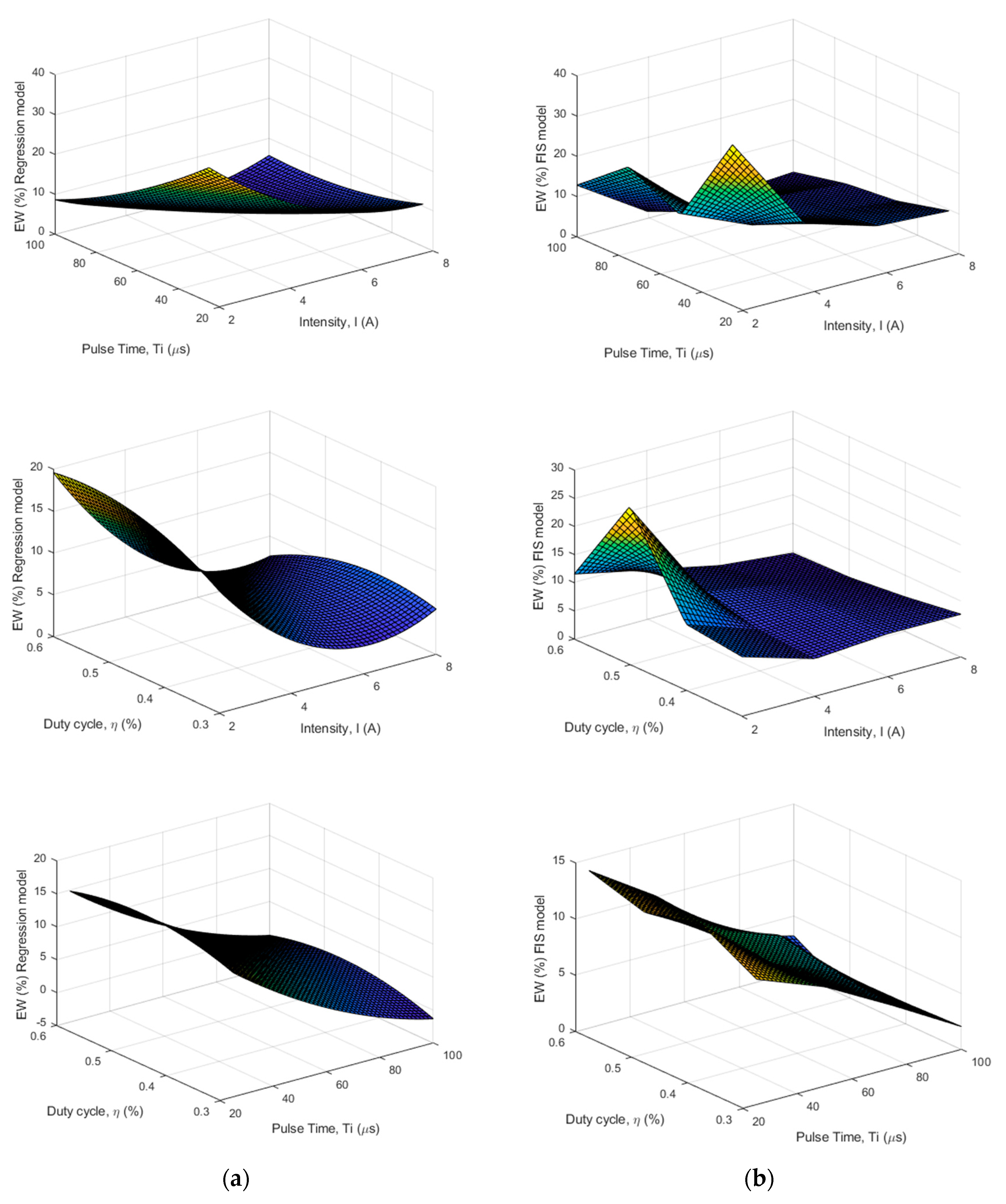
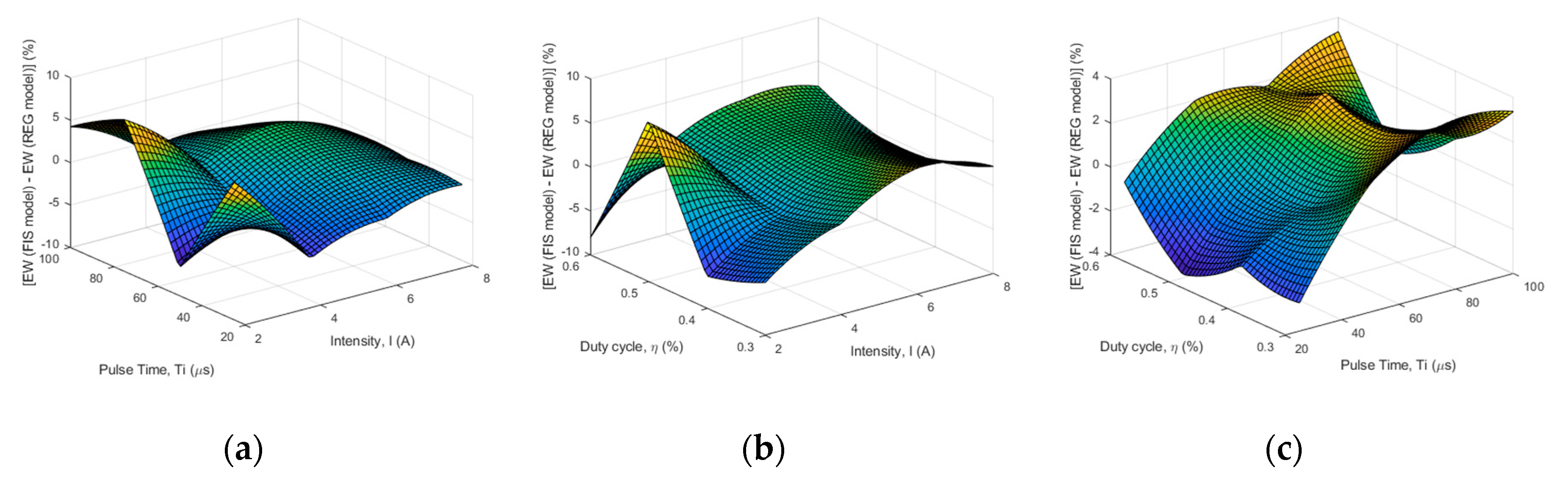
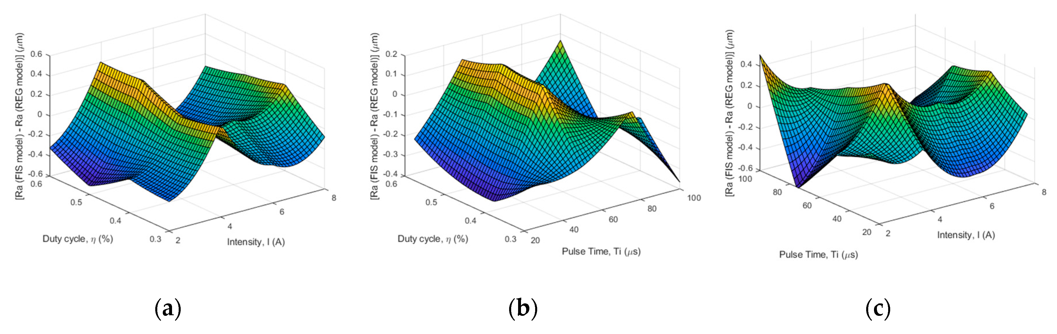
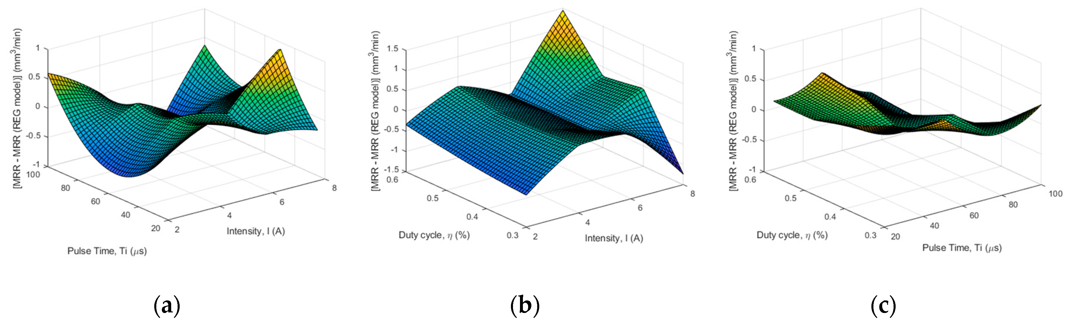
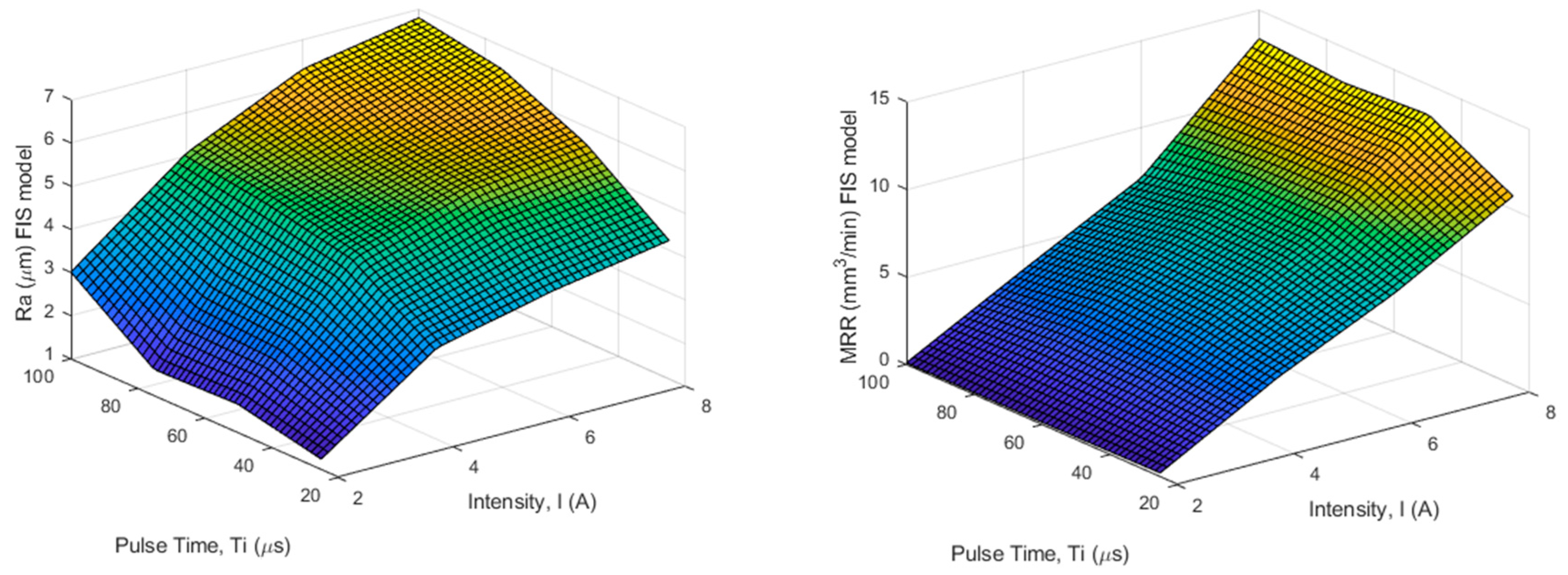
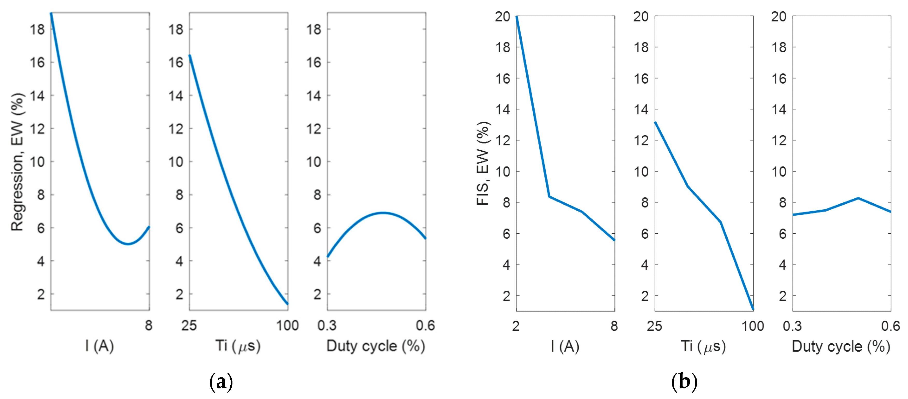
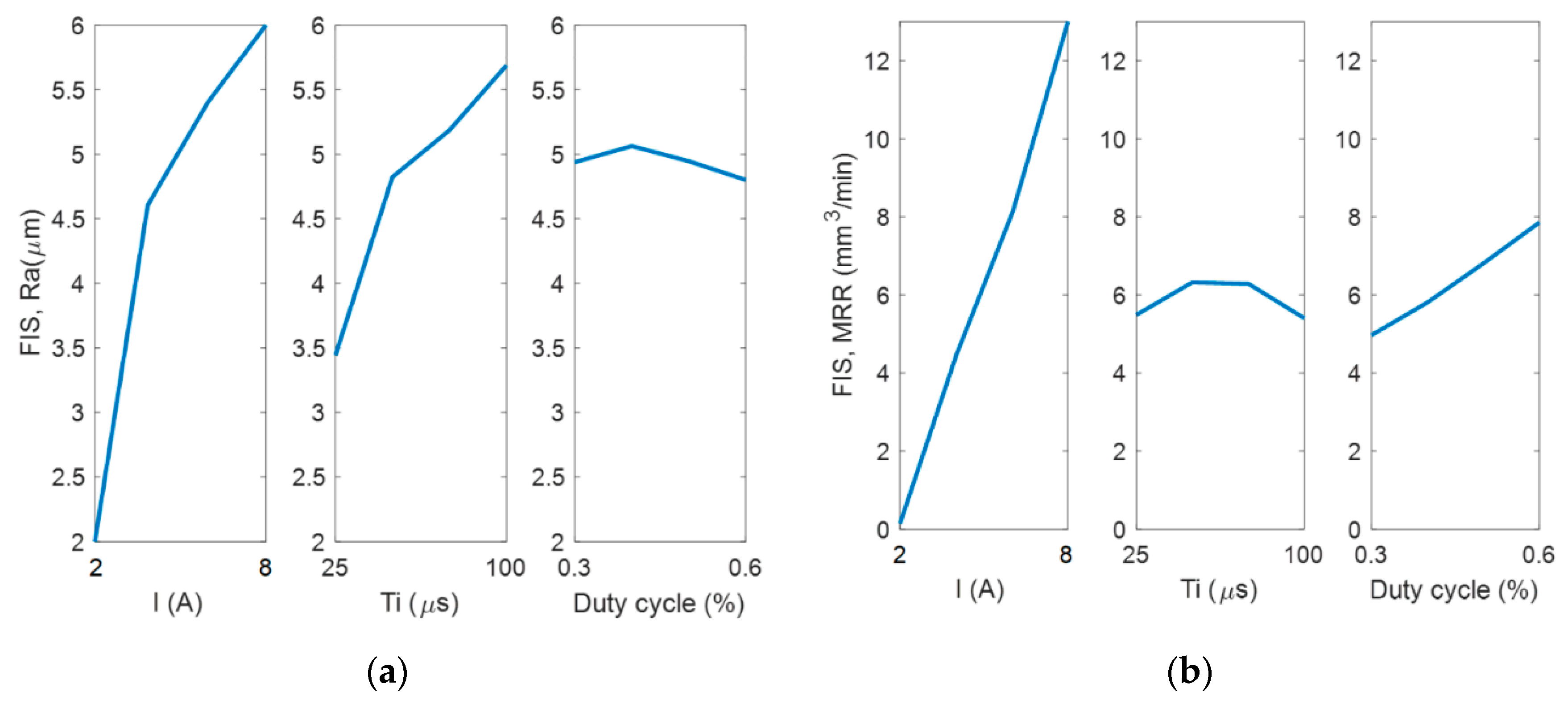
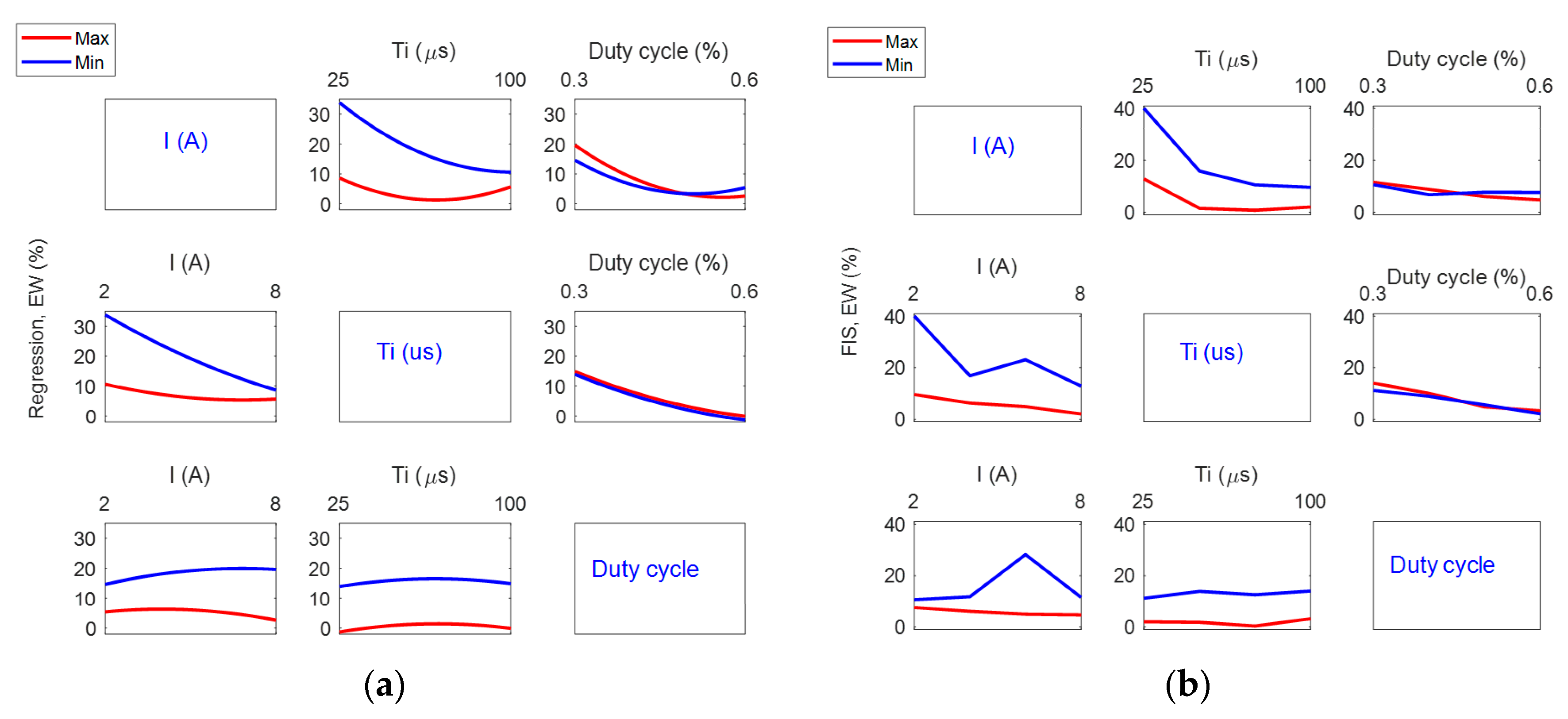
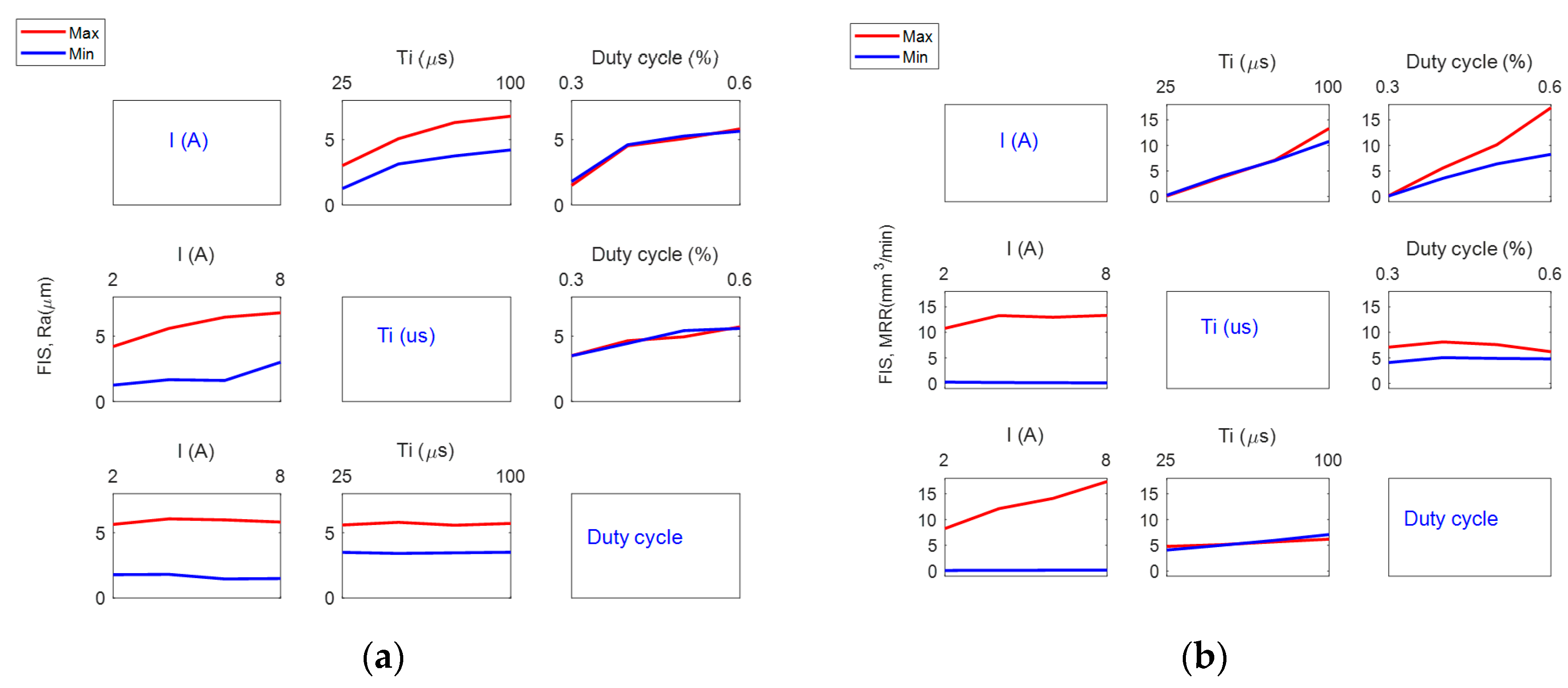
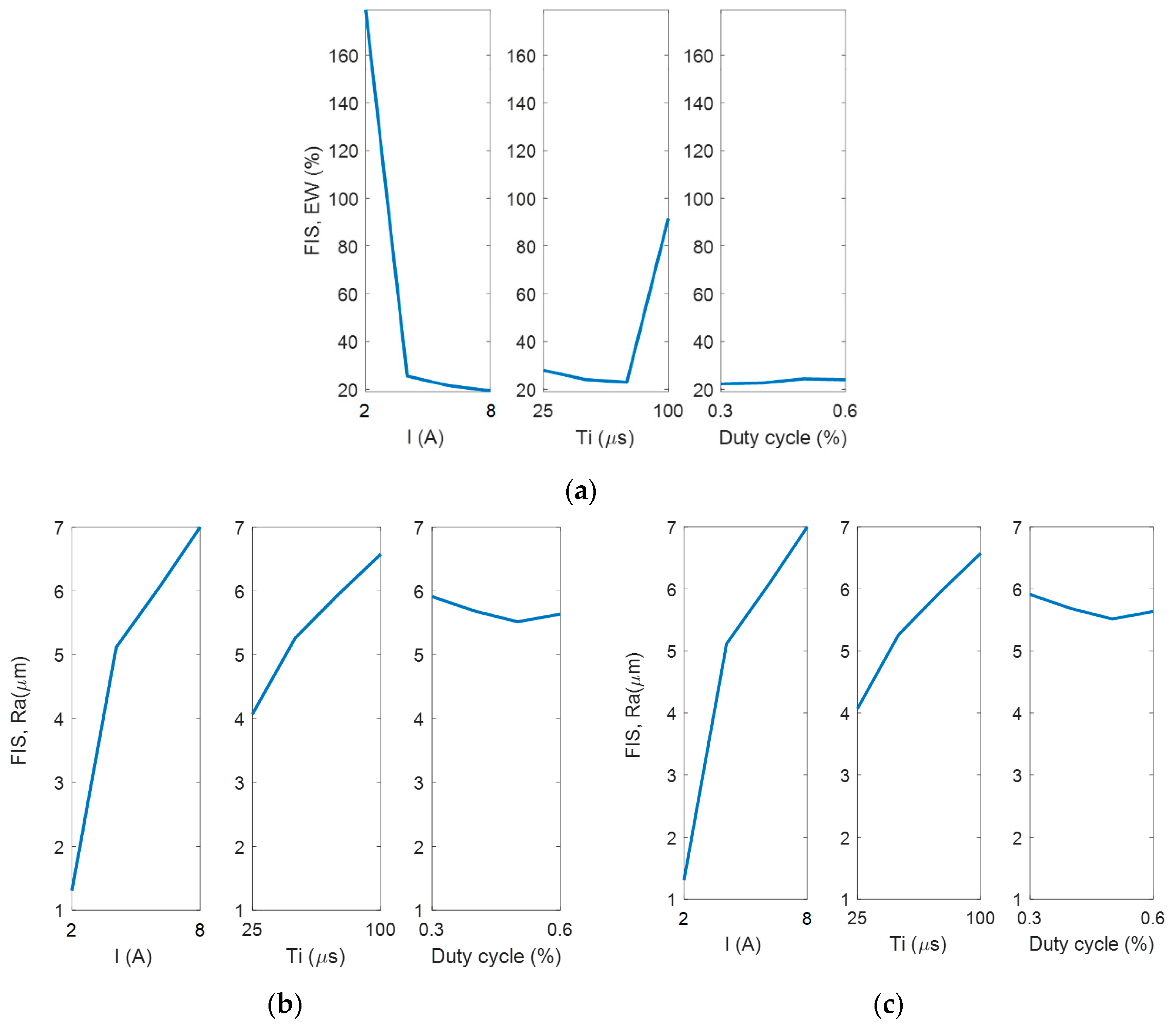
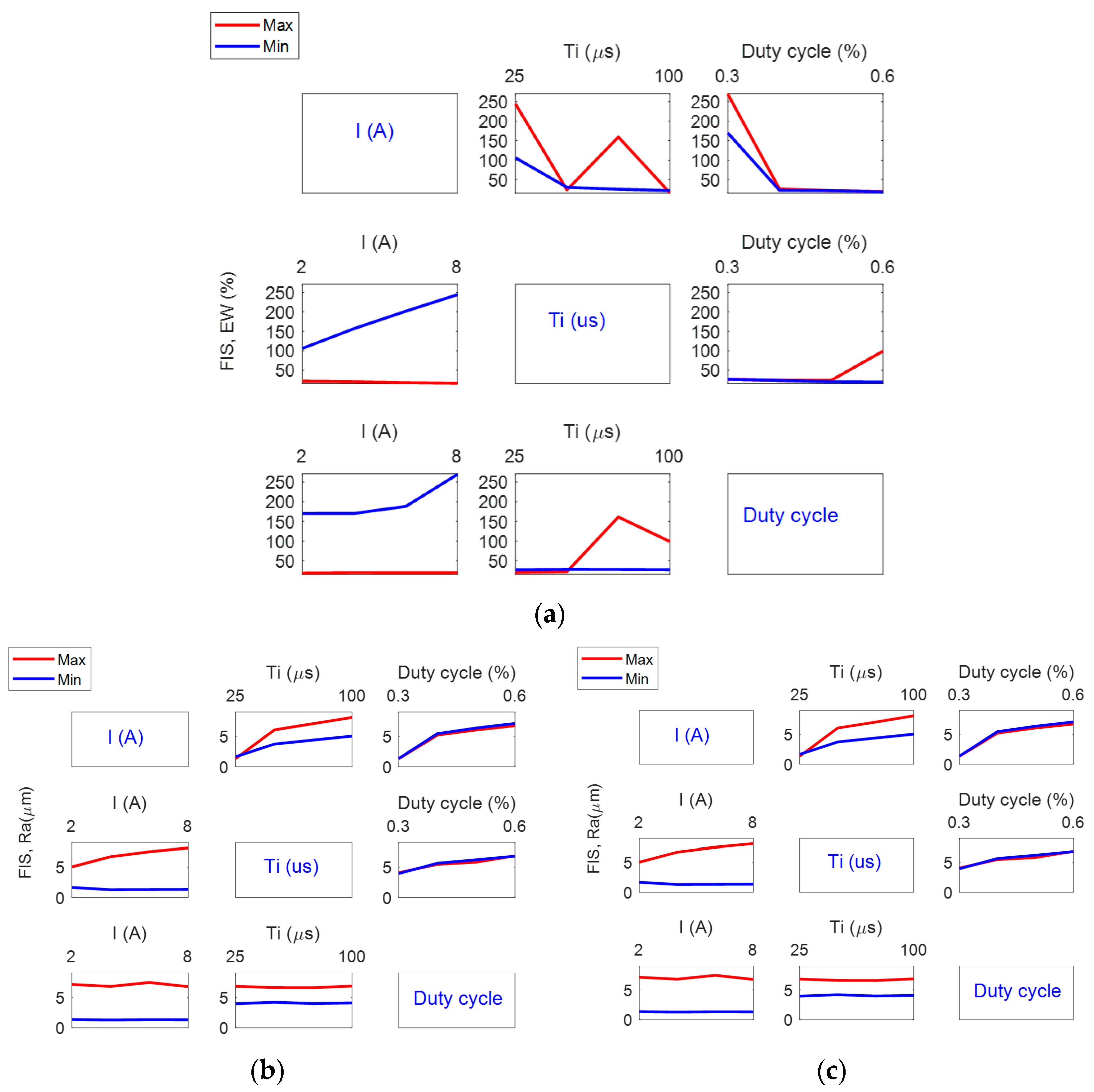
4.1. Analysis of Experimentation Using the FIS

This section is included in order to demonstrate that the FIS is able to model the behavior of the response variables more efficiently than by using RSM. Data shown in Table 1 and Table 2 are employed in order to develop a FIS which can be then employed to obtain the technological tables following the procedure previously mentioned in Section 3. As can be seen in Reference [1], a method for obtaining the technological tables from a conventional design of experiments along with multiple linear regression techniques was proposed, where technological tables were obtained for TiB₂, which is a sintered ceramic material and in Reference [5] technological tables were obtained for B₄C, SiSiC and WC-Co. However, as was previously mentioned, if the regression is not able to adequately predict the behavior of a response variable, the technological tables obtained from these models will not be accurate. In this section, the proposed methodology in this present study is applied for the case of the EDM of Inconel^® 600. However, it should be mentioned that this methodology could be applied for other kinds of materials. Figure 1 shows the membership functions that were used to fuzzify the inputs. As can be observed, triangular functions were selected for the inputs. On the other hand, the present study assumes that it is possible to linearly vary the parameters in the EDM equipment in order to be able to select the values obtained from the technological tables which are determined to be optimal ones. If this is not possible, the FIS would have to be used on the possible values of these independent variables. As Table 2 shows, the design of experiments does not continuously vary the values of the independent variables; thus, it is possible that the optimal values are not selected if only these values are considered. In addition, it may be that there are levels vacant when establishing the levels of roughness, which is the dependent variable that was selected as ${\mathrm{output}}_1$ since, as explained above, it is one of the most widely used parameters for characterizing surface quality and, therefore, its determination is of great importance and interest in industry.

In this present study, the FIS was obtained using Matlab™2019b. Therefore, from Table 2, it is possible to directly obtain the set of rules that make up the FIS. As previously mentioned, a Sugeno FIS was employed by using the Fuzzy Logic Toolbox™ of Matlab^TM2019b [40]. Mamdani systems are more intuitive and the rules are easier to understand, making them more suitable for expert systems, developed from human knowledge [40,42,43]. On the other hand, the defuzzification process for a Sugeno system is more computationally efficient compared to that of a Mamdani system [40,42,43]. Figure 4 shows the employed FIS which was developed from the rules shown in

Table 3. Codification of the rules.

$111,1\left(1\right) :1$	$1 1 2, 17 \left(1\right) : 1$	$1 1 3, 33 \left(1\right) : 1$	$1 1 4, 49 \left(1\right) : 1$
$2 1 1, 2 \left(1\right) : 1$	$2 1 2, 18 \left(1\right) : 1$	$2 1 3, 34 \left(1\right) : 1$	$2 1 4, 50 \left(1\right) : 1$
$3 1 1, 3 \left(1\right) : 1$	$3 1 2, 19 \left(1\right) : 1$	$3 1 3, 35 \left(1\right) : 1$	$3 1 4, 51 \left(1\right) : 1$
$4 1 1, 4 \left(1\right) : 1$	$4 1 2, 20 \left(1\right) : 1$	$4 1 3, 36 \left(1\right) : 1$	$4 1 4, 52 \left(1\right) : 1$
$1 2 1, 5 \left(1\right) : 1$	$1 2 2, 21 \left(1\right) : 1$	$1 2 3, 37 \left(1\right) : 1$	$1 2 4, 53 \left(1\right) : 1$
$2 2 1, 6 \left(1\right) : 1$	$2 2 2, 22 \left(1\right) : 1$	$2 2 3, 38 \left(1\right) : 1$	$2 2 4, 54 \left(1\right) : 1$
$3 2 1, 7 \left(1\right) : 1$	$3 2 2, 23 \left(1\right) : 1$	$3 2 3, 39 \left(1\right) : 1$	$3 2 4, 55 \left(1\right) : 1$
$4 2 1, 8 \left(1\right) : 1$	$4 2 2, 24 \left(1\right) : 1$	$4 2 3, 40 \left(1\right) : 1$	$4 2 4, 56 \left(1\right) : 1$
$1 3 1, 9 \left(1\right) : 1$	$1 3 2, 25 \left(1\right) : 1$	$1 3 3, 41 \left(1\right) : 1$	$1 3 4, 57 \left(1\right) : 1$
$2 3 1, 10 \left(1\right) : 1$	$2 3 2, 26 \left(1\right) : 1$	$2 3 3, 42 \left(1\right) : 1$	$2 3 4, 58 \left(1\right) : 1$
$3 3 1, 11 \left(1\right) : 1$	$3 3 2, 27 \left(1\right) : 1$	$3 3 3, 43 \left(1\right) : 1$	$3 3 4, 59 \left(1\right) : 1$
$4 3 1, 12 \left(1\right) : 1$	$4 3 2, 28 \left(1\right) : 1$	$4 3 3, 44 \left(1\right) : 1$	$4 3 4, 60 \left(1\right) : 1$
$1 4 1, 13 \left(1\right) : 1$	$1 4 2, 29 \left(1\right) : 1$	$1 4 3, 45 \left(1\right) : 1$	$1 4 4, 61 \left(1\right) : 1$
$2 4 1, 14 \left(1\right) : 1$	$2 4 2, 30 \left(1\right) : 1$	$2 4 3, 46 \left(1\right) : 1$	$2 4 4, 62 \left(1\right) : 1$
$3 4 1, 15 \left(1\right) : 1$	$3 4 2, 31 \left(1\right) : 1$	$3 4 3, 47 \left(1\right) : 1$	$3 4 4, 63 \left(1\right) : 1$
$4 4 1, 16 \left(1\right) : 1$	$4 4 2, 32 \left(1\right) : 1$	$4 4 3, 48 \left(1\right) : 1$	$4 4 4, 64 \left(1\right) : 1$

. This table shows the rules implemented in the fuzzy system, in symbolic format, codified from the outputs. For each output value, a FIS was developed. In this way, it is possible to model the behavior of Ra, MRR, and EW for each of the manufacturing strategies.

The codification shown in Table 3, which was obtained from Table 2, is “current intensity, pulse time, and duty cycle”: $“I\left(i\right) Ti\left(j\right) dc\left(k\right), \mathrm{output} \left(1=and, 2=or\right) : weight”$. In this case, $weight=1$, so that each rule has the same effect relative to others [40], where the numbering 1, 2, 3, and 4 is employed for the inputs in order to select the levels of the variables. As can be observed in Table 1, these variables have four levels. For example, the levels for the intensity are given by {2 A, 4 A, 6 A, and 8 A}. Therefore, these values are coded as {1, 2, 3, and 4} in Table 3. The same procedure is applied for both pulse time and duty cycle. In the case of the output, there are 64 values which are obtained from the DOE with the different input conditions. That is, for the case of Ra, for instance, $1 1 1,1 \left(1\right):1$ corresponds to the following:

$$1.\mathrm{If}\left(Intensity is 2\mathrm{A}\right)\mathrm{AND}\left(Pulse Time\mathrm{is}25\mathsf{\mu }\mathrm{s}\right)\mathrm{AND}\left(duty cycle\mathrm{is}0.3\%\right)\mathrm{THEN}\left(\mathrm{Ra} is 1.39 \mu \mathrm{m}\right).$$

That is,

$$\begin{gathered} 1.\mathrm{If}\left(I==I2\right)\&\left(Ti==Ti25\right)\&\left(dc==dc0.3\right)\mathrm{Then}\left(\mathrm{Output}=mf1\right), \\ 2.\mathrm{If}\left(I==I4\right)\&\left(Ti==Ti25\right)\&\left(dc==dc0.3\right)\mathrm{Then}\left(\mathrm{Output}=mf2\right), \\ 63.\mathrm{If}\left(I==I6\right)\&\left(Ti==Ti100\right)\&\left(dc==dc0.6\right)\mathrm{Then}\left(\mathrm{Output}=mf63\right), \\ 64.\mathrm{If}\left(I==I8\right)\&\left(Ti==Ti100\right)\&\left(dc==dc0.6\right)\mathrm{Then}\left(\mathrm{Output}=mf64\right), \end{gathered}$$

where the input values $“I\left(i\right),Ti\left(j\right),dc\left(k\right)”$ and the outputs $m{f}_1\dots m{f}_n$ are selected from Table 1.

$\mathrm{RSM} model:$

$$\begin{gathered} y ~ (b_0+b_1\times x_1+b_2\times x_2+b_3\times x_3+b_4\times x_1\times x_2+b_5\times x_1\times x_3+ \\ {b}_6\times x_2\times x_3+b_7\times x_1^2+b_8\times x_2^2+b_9\times x_3^2). \end{gathered}$$

(6)

The FIS was generated directly from experimental data. Therefore, as shown later, the precision of the obtained results is much higher than that obtained using RSM. Figure 5, Figure 6, Figure 7 and Figure 8 are included to compare the response surfaces obtained with the proposed methodology using the FIS and those obtained from the RSM, as done in Reference [2], where the experimental data were fitted by using a second degree polynomial, which is shown by Equation (6).

As can be observed in Figure 7 and Figure 8, the results obtained with the FIS are close to those obtained with the regression as a consequence of Ra and MRR being fitted adequately by a quadratic polynomial, as can be seen from the coefficients of determination of the fit and from the RMSE and mean absolute error (MAE) statistics, which are shown in Equation (7) and in

Table 4. Accuracy for predicted values of Ra, MRR, and EW using the regression model [2] and the FIS.

Positive Polarity (+)		Negative Polarity (−)
$\mathrm{Ra}$	$\mathrm{Ra}$	$\mathrm{Ra}$	$\mathrm{Ra}$
$\left(\mathrm{using}\mathrm{the}\mathrm{FIS}\right)$	$\left(\mathrm{Regression}\right)$	$\left(\mathrm{using}\mathrm{the}\mathrm{FIS}\right)$	$\left(\mathrm{Regression}\right)$
$\mathrm{RMSE}=0$	$\mathrm{RMSE}=0.3286$	$\mathrm{RMSE}=0$	$\mathrm{RMSE}=0.4461$
$\mathrm{MAE}=0$	$\mathrm{MAE}=0.2693$	$\mathrm{MAE}=0$	$\mathrm{MAE}=0.3705$
${\mathrm{R}}^2=1$	${\mathrm{R}}^2=0.9639$	${\mathrm{R}}^2=1$	${\mathrm{R}}^2=0.9606$
$\mathrm{MRR}$	$\mathrm{MRR}$	$\mathrm{MRR}$	$\mathrm{MRR}$
$\left(\mathrm{using}\mathrm{the}\mathrm{FIS}\right)$	$\left(\mathrm{Regression}\right)$	$\left(\mathrm{using}\mathrm{the}\mathrm{FIS}\right)$	$\left(\mathrm{Regression}\right)$
$\mathrm{RMSE}=0$	$\mathrm{RMSE}=0.7184$	$\mathrm{RMSE}=0$	$\mathrm{RMSE}=1.4713$
$\mathrm{MAE}=0$	$\mathrm{MAE}=0.4879$	$\mathrm{MAE}=0$	$\mathrm{MAE}=1.0625$
${\mathrm{R}}^2=1$	${\mathrm{R}}^2=0.9778$	${\mathrm{R}}^2=1$	${\mathrm{R}}^2=0.9712$
$\mathrm{EW}$	$\mathrm{EW}$	$\mathrm{EW}$	$\mathrm{EW}$
$\left(\mathrm{using}\mathrm{the}\mathrm{FIS}\right)$	$\left(\mathrm{Regression}\right)$	$\left(\mathrm{using}\mathrm{the}\mathrm{FIS}\right)$	$\left(\mathrm{Regression}\right)$
$\mathrm{RMSE}=0$	$\mathrm{RMSE}=5.5290$	$\mathrm{RMSE}=0$	$\mathrm{RMSE}=49.7581$
$\mathrm{MAE}=0$	$\mathrm{MAE}=3.5873$	$\mathrm{MAE}=0$	$\mathrm{MAE}=33.3053$
${\mathrm{R}}^2=1$	${\mathrm{R}}^2=0.6958$	${\mathrm{R}}^2=1$	${\mathrm{R}}^2=0.6783$

. However, as Table 4 shows, this is not the case for the electrode wear (EW), which is shown in Figure 5; hence, it is possible to conclude that the FIS is more accurate than RSM. Therefore, it is able to predict more adequately the values of the response, within the range of study, than the RSM.

Figure 6, Figure 7 and Figure 8 show a comparison between the EW, Ra, and MRR results obtained with the RSM and with the FIS. As can be observed in Figure 7 and Figure 8, differences are not significant as a consequence of the fact that experimental Ra and MRR results are well fitted by a second-order polynomial, such as that shown in Equation (6). However, this is not the case for electrode wear, as shown in Figure 5 and Figure 6. As Table 4 shows, the polynomial model is not accurate and, in this case, the differences between the FIS and the regression model are significant. Therefore, data provided by the FIS are more accurate than those obtained by using the RSM, and the technological tables are more accurate if the FIS is used instead of the regression model.

Figure 9 shows the response surfaces for both Ra and MRR obtained with the proposed methodology using the FIS for the case of positive polarity. Equation (7) shows the statistical parameters that were used to determine the precision of the models used for modeling the dependent variables, that is, Ra, MRR, and EW. As can be observed in Table 4, the FIS accuracy is higher than that provided by the RSM. Data shown in Table 4 were obtained by using Matlab™2019b.

$$\mathrm{RMSE}=\sqrt{\frac{1}{n}{\displaystyle \sum }_{j=1}^n{\left(y_j-{\widehat{y}}_j\right)}^2} and \mathrm{MAE}=\frac{1}{n}{\displaystyle \sum }_{j=1}^n\left|y_j-{\widehat{y}}_j\right|.$$

(7)

As can be observed in Table 4, the fuzzy inference system fits all the data perfectly, which is logical since the FIS was built according to the procedure shown in the previous section. However, this is not the case with the RSM which, despite using all the DOE points for the determination of the models, is not able to adequately adjust the electrode wear surface response. Therefore, the values predicted by the regression have lower accuracy than those predicted by the FIS. In this case, the polynomial models for the case of both roughness and material removal rate are acceptable. Nevertheless, the precision is lower than that of the FIS. In any case, in other types of experimentation in which there is less precision in the least squares adjustments, the employment of the FIS becomes more important since it adjusts to all the points of the model.

In Torres et al. [2], the model with the highest value of $adjusted R^2$ was selected. However, in this present study, the model with all the regression coefficients is used because these models have higher $R^2$ values than those shown in Reference [2] and, with the aim of considering all the effects in the models such as the models shown in Reference [2], some of the independent variables could be eliminated.

Figure 10b shows that it is possible to analyze the experimental results in a similar way to that done with regression models. It is shown that the most important effects are the current intensity and the pulse time, followed to a lesser extent by the duty cycle. In addition, by using the FIS, the values obtained are more precise, as can be seen in Table 4. As can be observed, the differences between the values predicted by the regression model and those predicted by the FIS are significant. Specifically, in the case of positive polarity, the regression model does not adequately predict the behavior of electrode wear, as can be seen in Table 4. Therefore, the results provided by the regression model when predicting electrode wear are not accurate. In this case, the FIS is shown to have significant advantages over the regression model. Specifically, it is shown that, with increasing intensity, there is less wear on the electrode, which is logical because, as seen in Figure 11a,b, if the intensity decreases, so does the removal of material, while the surface roughness assumes smaller values, with the wear of the electrode in these cases being greater, which is in good agreement with experimental values. Finally, Figure 12 shows the interaction effects plot. As can be observed, the most significant interactions are those related to the current intensity and the pulse time. On the other hand, it is observed that the differences between both the FIS and the regression are significant, as a consequence of the fact that the regression model is not able to adequately predict the behavior of the electrode wear. In addition, Table 4 shows that the FIS is able to predict the behavior of the response variables more adequately than the regression, which is logical as a consequence of the methodology employed for defining the FIS. Hence, the fit is perfect in the case of the FIS, and this is not so in the case of the regression model. Therefore, the technological tables with values provided by the FIS are more accurate than those provided by conventional methods.

Figure 11 shows that the current intensity is the variable that has the greatest impact on both Ra and MRR, which is logical since, within the values considered in the present study, a higher intensity reflects higher material removal and worse surface roughness. On the other hand, it can be observed in Figure 11b that the pulse time affects the material removal rate to only a slight extent and that, approximately for values of the pulse time within the range $50 \mathsf{\mu }\mathrm{s}<Ti \left(\mathsf{\mu }\mathrm{s}\right)<75 \mathsf{\mu }\mathrm{s}$, the material removal rate stands at its maximum value, being constant when the current intensity and the duty cycle are at their average values.

Figure 12$b_{\left(3x3\right)}$ shows that it is possible to analyze the interaction effects between factors by using the FIS in a similar way to conventional analysis of factorial 2^k experiments along with regression models. These factors are represented in an array $\left(3 files\times 3 columns\right)$. The results were generated by analyzing the variation of one factor between its maximum and minimum levels, when all the other factors were held at their average level. For example, in Figure 12 $b_{\left(1,2\right)}$, it is shown that, when the current intensity is held at its lowest level, the electrode wear values are lower with increasing pulse time, when the duty cycle is at its average level of 0.45%. Moreover, if the current intensity is held at its highest level, the electrode wear values are lower than those obtained when the current intensity is held at its lower level. On the other hand, in the case of duty cycle, which is represented in Figure 12 $b_{\left(1,3\right)}$, it is shown that the electrode wear remains approximately constant versus the duty cycle when the pulse time is held at a constant value of 62.5 µs, showing that the electrode wear values are independent of either higher or lower values of intensity. A similar analysis could be done with all the interaction effects. Figure 13 shows the interaction plots effect, using the FIS, for the three independent variables under study in the case of positive polarity when Ra and MRR are considered as response variables.

Figure 14 and Figure 15 show the main effects plot and the interaction effects plot for the case of negative polarity, using the FIS. As can be observed, a similar behavior to that of positive polarity is obtained. The same comments regarding the precision of the models are applicable in the negative polarity case.

As demonstrated in this section, the response surfaces generated with the FIS have greater precision than those obtained with the RSM; thus, the technological tables are determined according to the methodology described in the previous Section. It should be mentioned that it was considered necessary to develop the previous analysis in order to show the higher accuracy of the FIS model to predict the surface roughness, the material removal rate, and the wear of the electrode.

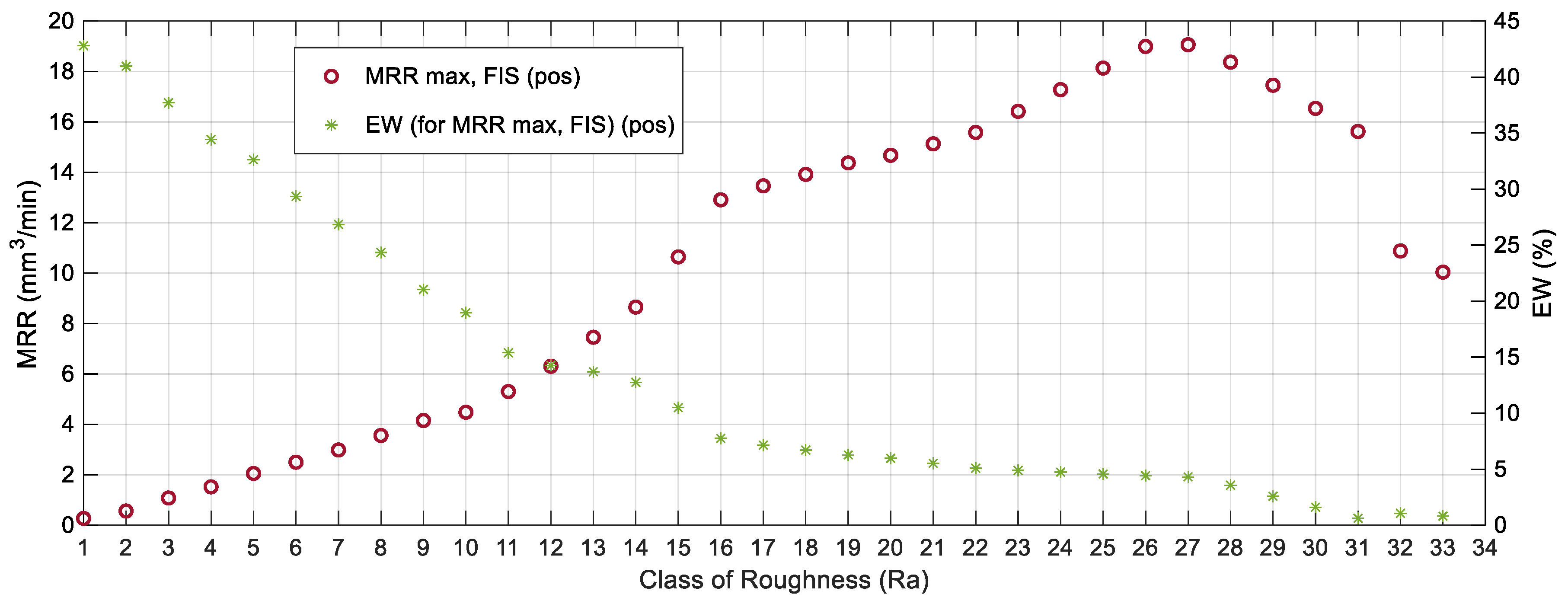
4.2. Development of the Technological Tables

In this section, the technological tables for the Inconel^® 600 alloy are obtained from the methodology previously described in Section 3. As can be observed in

Table 5. Strategy of maximum material removal rate. Technological table obtained from the FIS, for the case of maximum removal rate strategy (positive polarity).

Class of Roughness	$\mathrm{Lower}\mathrm{Value}\left(\mathsf{\mu }m\right)$	$\mathrm{Ra}\mathrm{Value}\left(\mathsf{\mu }m\right)$	$\mathrm{Upper}\mathrm{Value}\left(\mathsf{\mu }m\right)$	Intensity (A)	$\mathrm{Pulse}\mathrm{Time}\left(\mathsf{\mu }s\right)$	Duty Cycle (%)	$\mathrm{MRR}\mathrm{Max}\left(\frac{m{m}^3}{\min }\right)$	EW $\left(\mathit{\%}\right)$
$\mathrm{Ra}1$	$1.00$	$1.19$	$1.20$	$2.00$	$25.00$	$0.51$	$0.27$	$42.80$
$\mathrm{Ra}2$	$1.20$	$1.40$	$1.40$	$2.12$	$25.00$	$0.57$	$0.56$	$40.97$
$\mathrm{Ra}3$	$1.40$	$1.59$	$1.60$	$2.37$	$25.00$	$0.54$	$1.08$	$37.71$
$\mathrm{Ra}4$	$1.60$	$1.79$	$1.80$	$2.61$	$25.00$	$0.51$	$1.52$	$34.43$
$\mathrm{Ra}5$	$1.80$	$2.00$	$2.00$	$2.73$	$25.00$	$0.59$	$2.05$	$32.62$
$\mathrm{Ra}6$	$2.00$	$2.20$	$2.20$	$2.98$	$25.00$	$0.56$	$2.50$	$29.35$
$\mathrm{Ra}7$	$2.20$	$2.39$	$2.40$	$3.10$	$26.53$	$0.60$	$2.98$	$26.84$
$\mathrm{Ra}8$	$2.40$	$2.57$	$2.60$	$3.35$	$25.00$	$0.60$	$3.56$	$24.34$
$\mathrm{Ra}9$	$2.60$	$2.79$	$2.80$	$3.59$	$25.00$	$0.60$	$4.15$	$21.03$
$\mathrm{Ra}10$	$2.80$	$2.97$	$3.00$	$3.71$	$26.53$	$0.60$	$4.48$	$18.96$
$\mathrm{Ra}11$	$3.00$	$3.20$	$3.20$	$4.08$	$25.00$	$0.60$	$5.30$	$15.39$
$\mathrm{Ra}12$	$3.20$	$3.40$	$3.40$	$4.69$	$25.00$	$0.58$	$6.31$	$14.26$
$\mathrm{Ra}13$	$3.40$	$3.57$	$3.60$	$5.18$	$25.00$	$0.60$	$7.46$	$13.70$
$\mathrm{Ra}14$	$3.60$	$3.78$	$3.80$	$5.80$	$25.00$	$0.60$	$8.65$	$12.75$
$\mathrm{Ra}15$	$3.80$	$3.99$	$4.00$	$6.78$	$25.00$	$0.60$	$10.65$	$10.50$
$\mathrm{Ra}16$	$4.00$	$4.19$	$4.20$	$7.88$	$25.00$	$0.60$	$12.91$	$7.75$
$\mathrm{Ra}17$	$4.20$	$4.36$	$4.40$	$8.00$	$28.06$	$0.60$	$13.46$	$7.15$
$\mathrm{Ra}18$	$4.40$	$4.58$	$4.60$	$8.00$	$32.65$	$0.60$	$13.92$	$6.71$
$\mathrm{Ra}19$	$4.60$	$4.80$	$4.80$	$8.00$	$37.24$	$0.60$	$14.37$	$6.26$
$\mathrm{Ra}20$	$4.80$	$4.94$	$5.00$	$8.00$	$40.31$	$0.60$	$14.67$	$5.97$
$\mathrm{Ra}21$	$5.00$	$5.17$	$5.20$	$8.00$	$44.90$	$0.60$	$15.13$	$5.53$
$\mathrm{Ra}22$	$5.20$	$5.39$	$5.40$	$8.00$	$49.49$	$0.60$	$15.58$	$5.09$
$\mathrm{Ra}23$	$5.40$	$5.59$	$5.60$	$8.00$	$55.61$	$0.60$	$16.42$	$4.89$
$\mathrm{Ra}24$	$5.60$	$5.79$	$5.80$	$8.00$	$61.73$	$0.60$	$17.28$	$4.73$
$\mathrm{Ra}25$	$5.80$	$6.00$	$6.00$	$8.00$	$67.86$	$0.60$	$18.13$	$4.58$
$\mathrm{Ra}26$	$6.00$	$6.20$	$6.20$	$8.00$	$73.98$	$0.60$	$18.99$	$4.42$
$\mathrm{Ra}27$	$6.20$	$6.25$	$6.40$	$8.00$	$75.51$	$0.60$	$19.06$	$4.31$
$\mathrm{Ra}28$	$6.40$	$6.40$	$6.60$	$8.00$	$80.10$	$0.60$	$18.37$	$3.57$
$\mathrm{Ra}29$	$6.60$	$6.61$	$6.80$	$8.00$	$86.22$	$0.60$	$17.45$	$2.59$
$\mathrm{Ra}30$	$6.80$	$6.82$	$7.00$	$8.00$	$92.35$	$0.60$	$16.54$	$1.60$
$\mathrm{Ra}31$	$7.00$	$7.03$	$7.20$	$8.00$	$98.47$	$0.60$	$15.62$	$0.62$
$\mathrm{Ra}32$	$7.20$	$7.22$	$7.40$	$8.00$	$100.00$	$0.33$	$10.88$	$1.06$
$\mathrm{Ra}33$	$7.40$	$7.41$	$7.60$	$8.00$	$100.00$	$0.30$	$10.04$	$0.81$

,

Table 6. Strategy of minimum electrode wear. Technological table obtained from the FIS, for the case of minimum electrode wear strategy (positive polarity).

Class of Roughness	Lower Value (μm)	Ra Value (μm)	Upper Value (μm)	Intensity (A)	Pulse Time (μs)	Duty Cycle (%)	EW Min (%)	MRR $\mathbf{\left(}\frac{\mathbf{m}{\mathbf{m}}^{\mathbf{3}}}{\mathbf{min}}\mathbf{\right)}$
$\mathrm{Ra}1$	$1.00$	$1.20$	$1.20$	$2.00$	$26.53$	$0.50$	$40.93$	$0.26$
$\mathrm{Ra}2$	$1.20$	$1.40$	$1.40$	$2.00$	$52.55$	$0.60$	$16.57$	$0.18$
$\mathrm{Ra}3$	$1.40$	$1.59$	$1.60$	$2.00$	$72.45$	$0.60$	$6.48$	$0.14$
$\mathrm{Ra}4$	$1.60$	$1.80$	$1.80$	$2.00$	$90.82$	$0.60$	$3.20$	$0.11$
$\mathrm{Ra}5$	$1.80$	$1.99$	$2.00$	$2.00$	$75.51$	$0.31$	$1.03$	$0.09$
$\mathrm{Ra}6$	$2.00$	$2.02$	$2.20$	$2.00$	$75.51$	$0.30$	$0.49$	$0.08$
$\mathrm{Ra}7$	$2.20$	$2.21$	$2.40$	$2.12$	$75.51$	$0.30$	$0.73$	$0.28$
$\mathrm{Ra}8$	$2.40$	$2.43$	$2.60$	$2.24$	$77.04$	$0.30$	$1.09$	$0.48$
$\mathrm{Ra}9$	$2.60$	$2.61$	$2.80$	$2.37$	$77.04$	$0.30$	$1.31$	$0.68$
$\mathrm{Ra}10$	$2.80$	$2.82$	$3.00$	$2.49$	$78.57$	$0.30$	$1.63$	$0.87$
$\mathrm{Ra}11$	$3.00$	$3.12$	$3.20$	$2.73$	$75.51$	$0.30$	$1.89$	$1.28$
$\mathrm{Ra}12$	$3.20$	$3.21$	$3.40$	$2.73$	$80.10$	$0.30$	$2.12$	$1.25$
$\mathrm{Ra}13$	$3.40$	$3.49$	$3.60$	$2.98$	$75.51$	$0.30$	$2.36$	$1.68$
$\mathrm{Ra}14$	$3.60$	$3.67$	$3.80$	$3.10$	$75.51$	$0.30$	$2.59$	$1.88$
$\mathrm{Ra}15$	$3.80$	$3.85$	$4.00$	$3.22$	$75.51$	$0.30$	$2.82$	$2.08$
$\mathrm{Ra}16$	$4.00$	$4.01$	$4.20$	$3.22$	$89.29$	$0.30$	$3.00$	$1.90$
$\mathrm{Ra}17$	$4.20$	$4.21$	$4.40$	$3.35$	$93.88$	$0.30$	$3.12$	$2.02$
$\mathrm{Ra}18$	$4.40$	$4.41$	$4.60$	$3.47$	$100.00$	$0.30$	$3.16$	$2.10$
$\mathrm{Ra}19$	$4.60$	$4.79$	$4.80$	$3.84$	$100.00$	$0.40$	$3.02$	$3.11$
$\mathrm{Ra}20$	$4.80$	$5.00$	$5.00$	$3.84$	$100.00$	$0.49$	$1.86$	$3.61$
$\mathrm{Ra}21$	$5.00$	$5.19$	$5.20$	$4.08$	$100.00$	$0.48$	$0.76$	$4.02$
$\mathrm{Ra}22$	$5.20$	$5.36$	$5.40$	$4.45$	$100.00$	$0.50$	$0.47$	$4.72$
$\mathrm{Ra}23$	$5.40$	$5.55$	$5.60$	$4.94$	$100.00$	$0.50$	$0.43$	$5.59$
$\mathrm{Ra}24$	$5.60$	$5.79$	$5.80$	$5.55$	$100.00$	$0.50$	$0.37$	$6.63$
$\mathrm{Ra}25$	$5.80$	$5.94$	$6.00$	$5.92$	$100.00$	$0.50$	$0.33$	$7.26$
$\mathrm{Ra}26$	$6.00$	$6.00$	$6.20$	$6.04$	$100.00$	$0.50$	$0.37$	$7.49$
$\mathrm{Ra}27$	$6.20$	$6.21$	$6.40$	$6.04$	$100.00$	$0.47$	$0.62$	$7.34$
$\mathrm{Ra}28$	$6.40$	$6.58$	$6.60$	$6.65$	$100.00$	$0.30$	$0.83$	$7.84$
$\mathrm{Ra}29$	$6.60$	$6.79$	$6.80$	$7.27$	$100.00$	$0.59$	$0.76$	$12.74$
$\mathrm{Ra}30$	$6.80$	$6.99$	$7.00$	$7.76$	$100.00$	$0.60$	$0.48$	$14.54$
$\mathrm{Ra}31$	$7.00$	$7.08$	$7.20$	$8.00$	$100.00$	$0.60$	$0.37$	$15.39$
$\mathrm{Ra}32$	$7.20$	$7.33$	$7.40$	$7.88$	$100.00$	$0.30$	$0.81$	$9.84$
$\mathrm{Ra}33$	$7.40$	$7.41$	$7.60$	$8.00$	$100.00$	$0.30$	$0.81$	$10.04$

,

Table 7. Strategy of maximum material removal rate. Technological table obtained from the FIS, for the case of maximum removal rate strategy (negative polarity).

Class of Roughness	Lower Value (μm)	Ra Value (μm)	Upper Value (μm)	Intensity (A)	Pulse Time (μs)	Duty Cycle (%)	MRR Max $\mathbf{\left(}\frac{\mathbf{m}{\mathbf{m}}^{\mathbf{3}}}{\mathbf{min}}\mathbf{\right)}$	EW (%)
$\mathrm{Ra}2$	$1.20$	$1.39$	$1.40$	$2.00$	$44.90$	$0.50$	$0.51$	$145.31$
$\mathrm{Ra}3$	$1.40$	$1.60$	$1.60$	$2.24$	$25.00$	$0.60$	$1.76$	$219.37$
$\mathrm{Ra}4$	$1.60$	$1.80$	$1.80$	$2.37$	$29.59$	$0.60$	$2.48$	$212.79$
$\mathrm{Ra}5$	$1.80$	$1.99$	$2.00$	$2.49$	$31.12$	$0.60$	$3.21$	$201.03$
$\mathrm{Ra}6$	$2.00$	$2.18$	$2.20$	$2.61$	$32.65$	$0.60$	$3.94$	$188.91$
$\mathrm{Ra}7$	$2.20$	$2.37$	$2.40$	$2.86$	$25.00$	$0.60$	$5.26$	$153.08$
$\mathrm{Ra}8$	$2.40$	$2.60$	$2.60$	$2.98$	$28.06$	$0.60$	$6.02$	$142.45$
$\mathrm{Ra}9$	$2.60$	$2.76$	$2.80$	$3.10$	$28.06$	$0.60$	$6.73$	$128.83$
$\mathrm{Ra}10$	$2.80$	$2.98$	$3.00$	$3.35$	$25.00$	$0.60$	$8.07$	$100.04$
$\mathrm{Ra}11$	$3.00$	$3.19$	$3.20$	$3.47$	$26.53$	$0.60$	$8.81$	$87.37$.
$\mathrm{Ra}12$	$3.20$	$3.35$	$3.40$.	$3.59$	$26.53$.	$0.60$.	$9.51$	$73.93$
$\mathrm{Ra}13$	$3.40$	$3.60$	$3.60$	$3.84$	$25.00$	$0.60$	$10.87$	$47.01$
$\mathrm{Ra}14$	$3.60$	$3.75$	$3.80$	$3.96$	$25.00$	$0.60$	$11.57$	$33.75$
$\mathrm{Ra}15$	$3.80$	$3.98$	$4.00$	$4.69$	$25.00$	$0.60$	$14.20$	$27.80$
$\mathrm{Ra}16$	$4.00$	$4.18$	$4.20$	$5.43$	$25.00$	$0.60$	$16.73$	$26.18$
$\mathrm{Ra}17$	$4.20$	$4.35$	$4.40$	$6.04$	$25.00$	$0.60$	$18.94$	$24.86$
$\mathrm{Ra}18$	$4.40$	$4.57$	$4.60$	$6.53$	$25.00$	$0.60$	$21.78$	$24.13$
$\mathrm{Ra}19$	$4.60$	$4.79$	$4.80$	$7.02$	$25.00$	$0.60$	$24.63$	$23.39$
$\mathrm{Ra}20$	$4.80$	$4.96$	$5.00$	$7.39$	$25.00$	$0.60$	$26.76$	$22.85$
$\mathrm{Ra}21$	$5.00$	$5.18$	$5.20$	$7.88$	$25.00$	$0.60$	$29.60$	$22.11$
$\mathrm{Ra}22$	$5.20$	$5.39$	$5.40$	$8.00$	$28.06$	$0.60$	$30.33$	$21.62$
$\mathrm{Ra}23$	$5.40$	$5.55$	$5.60$	$8.00$	$31.12$	$0.60$	$30.35$	$21.31$
$\mathrm{Ra}24$	$5.60$	$5.78$	$5.80$	$8.00$	$35.71$	$0.60$	$30.38$	$20.84$
$\mathrm{Ra}25$	$5.80$	$5.93$	$6.00$	$8.00$	$38.78$	$0.60$	$30.40$	$20.52$
$\mathrm{Ra}26$	$6.00$	$6.17$	$6.20$	$8.00$	$43.37$	$0.60$	$30.43$	$20.06$
$\mathrm{Ra}27$	$6.20$	$6.40$	$6.40$	$8.00$	$47.96$	$0.60$	$30.46$	$19.59$
$\mathrm{Ra}28$	$6.40$	$6.47$	$6.60$	$8.00$	$49.49$	$0.60$	$30.47$	$19.43$
$\mathrm{Ra}29$	$6.60$	$6.61$	$6.80$	$8.00$	$55.61$	$0.60$	$29.23$	$19.40$
$\mathrm{Ra}30$	$6.80$	$6.80$	$7.00$	$8.00$	$63.27$	$0.59$	$27.19$	$19.41$
$\mathrm{Ra}31$	$7.00$	$7.19$	$7.20$	$7.76$	$83.16$	$0.60$	$26.19$	$25.20$
$\mathrm{Ra}32$	$7.20$	$7.39$	$7.40$	$7.88$	$87.76$	$0.60$	$27.44$	$23.36$
$\mathrm{Ra}33$	$7.40$	$7.57$	$7.60$	$8.00$	$92.35$	$0.60$	$28.78$	$18.10$
$\mathrm{Ra}34$	$7.60$	$7.78$	$7.80$	$8.00$	$98.47$	$0.60$	$30.15$	$17.61$
$\mathrm{Ra}35$	$7.80$	$7.83$	$8.00$	$8.00$	$100.00$	$0.60$	$30.49$	$17.49$
$\mathrm{Ra}36$	$8.00$	$8.01$	$8.20$	$8.00$	$100.00$	$0.56$	$28.07$	$16.96$
$\mathrm{Ra}37$	$8.20$	$8.23$	$8.40$.	$8.00$	$100.00$	$0.52$	$25.24$	$16.34$

and

Table 8. Strategy of minimum electrode wear. Technological table obtained from the FIS, for the case of minimum electrode wear strategy (negative polarity).

Class of Roughness	Lower Value (μm)	Ra Value (μm)	Upper Value (μm)	Intensity (A)	Pulse Time (μs)	Duty Cycle (%)	EW Min (%)	MRR $\mathbf{\left(}\frac{\mathbf{m}{\mathbf{m}}^{\mathbf{3}}}{\mathbf{min}}\mathbf{\right)}$
$\mathrm{Ra}2$	$1.20$	$1.39$	$1.40$	$2.00$	$41.84$	$0.30$	$138.16$	$0.37$
$\mathrm{Ra}3$	$1.40$	$1.57$	$1.60$	$2.00$	$25.00$	$0.30$	$96.67$	$0.50$
$\mathrm{Ra}4$	$1.60$	$1.69$	$1.80$	$2.12$	$25.00$	$0.30$	$92.48$	$0.76$
$\mathrm{Ra}5$	$1.80$	$1.94$	$2.00$	$2.37$	$25.00$	$0.30$	$84.10$	$1.29$
$\mathrm{Ra}6$	$2.00$	$2.19$	$2.20$	$2.61$	$25.00$	$0.30$	$75.72$	$1.81$
$\mathrm{Ra}7$	$2.20$	$2.31$	$2.40$	$2.73$	$25.00$	$0.30$	$71.53$	$2.08$
$\mathrm{Ra}8$	$2.40$	$2.56$	$2.60$	$2.98$	$25.00$	$0.30$	$63.15$	$2.60$
$\mathrm{Ra}9$	$2.60$	$2.68$	$2.80$	$3.10$	$25.00$	$0.30$	$58.96$	$2.86$
$\mathrm{Ra}10$	$2.80$	$2.93$	$3.00$	$3.35$	$25.00$	$0.30$	$50.58$	$3.39$
$\mathrm{Ra}11$	$3.00$	$3.18$	$3.20$	$3.59$	$25.00$	$0.30$	$42.20$	$3.92$
$\mathrm{Ra}12$	$3.20$	$3.30$	$3.40$	$3.71$	$25.00$	$0.30$	$38.01$	$4.18$
$\mathrm{Ra}13$	$3.40$	$3.55$	$3.60$	$3.96$	$25.00$	$0.30$	$29.63$	$4.71$
$\mathrm{Ra}14$	$3.60$	$3.79$	$3.80$	$4.57$	$25.00$	$0.30$	$27.56$	$5.31$
$\mathrm{Ra}15$	$3.80$	$3.96$	$4.00$	$5.06$	$25.00$	$0.30$	$26.99$	$5.75$
$\mathrm{Ra}16$	$4.00$	$4.20$	$4.20$	$5.55$	$25.00$	$0.58$	$26.05$	$16.12$
$\mathrm{Ra}17$	$4.20$	$4.40$	$4.40$	$6.16$	$25.00$	$0.59$	$24.77$	$18.85$
$\mathrm{Ra}18$	$4.40$	$4.59$	$4.60$	$7.27$	$25.00$	$0.30$	$22.86$	$9.02$
$\mathrm{Ra}19$	$4.60$	$4.76$	$3.40$	$4.80$	$8.00$	$0.30$	$21.09$	$10.42$
$\mathrm{Ra}20$	$4.80$	$4.88$	$5.00$	$8.00$	$26.53$	$0.30$	$20.97$	$10.66$
$\mathrm{Ra}21$	$5.00$	$5.13$	$5.20$	$8.00$	$29.59$	$0.30$	$20.72$	$11.14$
$\mathrm{Ra}22$	$5.20$	$5.38$	$5.40$	$8.00$	$32.65$	$0.30$	$20.47$	$11.62$
$\mathrm{Ra}23$	$5.40$	$5.54$	$5.60$	$4.08$	$75.51$	$0.30$	$20.02$	$7.91$
$\mathrm{Ra}24$	$5.60$	$5.64$	$5.80$	$4.08$	$78.57$	$0.30$	$20.05$	$8.20$
$\mathrm{Ra}25$	$5.80$	$5.99$	$6.00$	$8.00$	$40.31$	$0.30$	$19.84$	$12.82$
$\mathrm{Ra}26$	$6.00$	$6.11$	$6.20$	$8.00$	$41.84$	$0.30$	$19.72$	$13.06$
$\mathrm{Ra}27$	$6.20$	$6.36$	$6.40$	$8.00$	$44.90$	$0.30$	$19.47$	$13.54$
$\mathrm{Ra}28$	$6.40$	$6.48$	$6.60$	$8.00$	$46.43$	$0.30$	$19.34$	$13.78$
$\mathrm{Ra}29$	$6.60$	$6.80$	$6.80$	$7.02$	$75.51$	$0.40$	$18.82$	$17.61$
$\mathrm{Ra}30$	$6.80$	$7.00$	$7.00$	$7.51$	$73.98$	$0.40$	$18.37$	$19.49$
$\mathrm{Ra}31$	$7.00$	$7.16$	$7.20$	$7.76$	$75.51$	$0.40$	$17.93$	$20.47$
$\mathrm{Ra}32$	$7.20$	$7.36$	$7.40$	$8.00$	$78.57$	$0.40$	$17.53$	$21.59$
$\mathrm{Ra}33$	$7.40$	$7.59$	$7.60$	$8.00$	$87.76$	$0.40$	$17.23$	$22.07$
$\mathrm{Ra}34$	$7.60$	$7.79$	$7.80$	$8.00$	$95.41$	$0.40$	$16.98$	$22.47$
$\mathrm{Ra}35$	$7.80$	$8.00$	$8.00$	$8.00$	$100.00$	$0.42$	$16.65$	$23.02$
$\mathrm{Ra}36$	$8.00$	$8.18$	$8.20$	$8.00$	$100.00$	$0.47$	$16.31$	$23.50$
$\mathrm{Ra}37$	$8.20$	$8.32$	$8.40$	$8.00$	$100.00$	$0.50$	$16.07$	$24.03$

, $\mathrm{Ra}$ is classified with a pitch of $0.20 \mathsf{\mu }\mathrm{m}$. Although it would be possible to generate the technological tables only using the experimental data, it could be that there exist roughness classes in which there are no input variables to obtain them, since the dependent variables are obtained afterward and, therefore, their value is not known in advance. Moreover, it could happen that MRR and EW values were not optimized as a consequence of the fact that the inputs are not linearly varied in the DOE.

Table 5 shows the technological table for the case of positive polarity that was obtained by selecting a specific class of roughness values with the maximum values of the material removal rate. The electrode wear is given by the FIS after selecting the input variables that lead to a specific roughness value, and Table 6 shows the technological table for the case of minimum electrode wear. In this case, the material removal rate is obtained from the FIS once the input variables are defined.

In previous research studies, in which the author participated, technological tables were obtained using regression models [1,5]. However, as shown in the previous section, the FIS is capable of providing more precise values than those obtained by means of a conventional regression. Therefore, the methodology described in Section 3 was used in this present study to generate the technological tables. It should be mentioned that a pitch of $0.20 \mathsf{\mu }\mathrm{m}$ was selected for classifying $\mathrm{Ra}$. However, this value could be whatever without loss of generality. From the values shown in Table 1 and Table 2, an interval that encompasses both the minimum and the maximum values was selected. In this interval, the roughness classes are established from the selected pitch and, thus, the technological tables can then be obtained.

Figure 16 and Figure 17 show the values obtained from the technological table with the fuzzy inference system for the strategy of maximum material removal rate using positive and negative polarities, respectively. These figures were obtained from Table 5 and Table 7, respectively.

Figure 18 and Figure 19 show the values obtained from the technological table with the fuzzy inference system for the strategy of minimum electrode wear using positive and negative polarities, respectively. These figures were obtained from Table 6 and Table 8, respectively.

5. Conclusions

In this present study, a methodology that combines an experimental design with fuzzy modeling was used in order to obtain the technological tables that make it possible to select in advance the most suitable machining conditions in order to either maximize or minimize a certain objective function (in this case the material removal rate and wear of the electrode) in a process of EDM. In addition, a case study was analyzed for an Inconel^® alloy.

Knowledge of the technological tables is very important since it makes it possible to select a certain machining strategy, so that it is possible to obtain certain values of roughness along with maximum material removal or minimum electrode wear. It was shown that the fuzzy model is capable of generating the results in a more efficient way than that obtained by conventional regression techniques. Moreover, the fuzzy model has the advantage that it is easy to incorporate new rules into the model, in the event that there are additional experimental tests.

In this present study, it was shown that the FIS allows the behavior of the technological variables used in the EDM processes to be adequately modeled and that the statistical values provided by this methodology, which were quantified by RMSE, MAE, and R-squared, are much better than those obtained by conventional methods. Therefore, the use of a FIS to obtain the EDM technology tables may be an interesting alternative, due to the fact that higher precision can be obtained compared to that obtained by traditional RSM-based methodologies.

It is felt that the present methodology for obtaining the technological tables may be of interest in the event that the input variables to the EDM equipment can be varied continuously and, thus, it could be possible to select the most appropriate operating conditions in advance. Likewise, it is felt that the proposed methodology could be generally applied for any other material and for other manufacturing processes.

Finally, it should be mentioned that it would have been possible to perform a reverse approach, that is, to train the model from the experimental data in order to obtain an adaptive neuro-fuzzy inference system; then, the technological tables could have been obtained. This will be done in a future study.

References

1. Torres, A.; Luis, C.J.; Puertas, I. EDM machinability and surface roughness analysis of TiB2 using copper electrodes. J. Alloys Compd. 2017, 690, 337–347. [Google Scholar] [CrossRef]
2. Salcedo, A.T.; Puertas, I.; Luis Pérez, C.J. Analytical Modelling of Energy Density and Optimization of the EDM Machining Parameters of Inconel 600. Metals 2017, 7, 166. [Google Scholar] [CrossRef] [Green Version]
3. Nguyen, H.T.; Sugeno, M. Fuzzy Systems, Modeling and Control; Springer-Science+Businees Media: New York, NY, USA, 1998. [Google Scholar]
4. Takagi, T.; Sugeno, M. Fuzzy Identification of Systems and Its Applications to Modeling and Control. IEEE Trans. Syst. ManCybern. 1985, SMC-15, 116–132. [Google Scholar] [CrossRef]
5. Luis, C.J.; Puertas, I. Methodology for developing technological tables used in EDM processes of conductive ceramics. J. Mater. Process. Technol. 2007, 189, 301–309. [Google Scholar] [CrossRef]
6. Nguyen, A.T.; Taniguchi, T.; Eciolaza, L.; Campos, V.; Palhares, R.; Sugeno, R.M. Fuzzy Control Systems: Past, Present and Future. IEEE Comput. Intell. Mag. 2019, 14, 56–68. [Google Scholar] [CrossRef]
7. Mamdani, E.H. Application of fuzzy algorithms for control of simple dynamic plant. In Proceedings of the Institution of Electrical Engineers; Institution of Engineering and Technology (IET): Stevenage, UK, 1974; Volume 121, pp. 1585–1588. [Google Scholar]
8. Mamdani, E.H. Application of Fuzzy Logic to Approximate Reasoning Using Linguistic Synthesis. IEEE Trans. Comput. 1976, C-26, 1182–1191. [Google Scholar] [CrossRef]
9. Mouralova, K.; Hrabec, P.; Benes, L.; Otoupalik, J.; Bednar, J.; Prokes, T.; Matousek, R. Verification of Fuzzy Inference System for Cutting Speed while WEDM for the Abrasion-Resistant Steel Creusabro by Conventional Statistical Methods. Metals 2020, 10, 92. [Google Scholar] [CrossRef] [Green Version]
10. Aamir, M.; Tu, S.; Tolouei-Rad, M.; Giasin, K.; Vafadar, A. Optimization and Modeling of Process Parameters in Multi-Hole Simultaneous Drilling Using Taguchi Method and Fuzzy Logic Approach. Materials 2020, 13, 680. [Google Scholar] [CrossRef] [Green Version]
11. Alarifi, I.M.; Nguyen, H.M.; Naderi Bakhtiyari, A.; Asadi, A. Feasibility of ANFIS-PSO and ANFIS-GA Models in Predicting Thermophysical Properties of Al2O3-MWCNT/Oil Hybrid Nanofluid. Materials 2019, 12, 3628. [Google Scholar] [CrossRef] [Green Version]
12. Wang, C.-N.; Nguyen, V.T.; Chyou, J.-T.; Lin, T.-F.; Nguyen, T.N. Fuzzy Multicriteria Decision-Making Model (MCDM) for Raw Materials Supplier Selection in Plastics Industry. Mathematics 2019, 7, 981. [Google Scholar] [CrossRef] [Green Version]
13. Kang, H.; Cho, H.-C.; Choi, S.-H.; Heo, I.; Kim, H.-Y.; Kim, K.S. Estimation of Heating Temperature for Fire-Damaged Concrete Structures Using Adaptive Neuro-Fuzzy Inference System. Materials 2019, 12, 3964. [Google Scholar] [CrossRef] [PubMed] [Green Version]
14. Tayyab, M.; Sarkar, B.; Yahya, B.N. Imperfect Multi-Stage Lean Manufacturing System with Rework under Fuzzy Demand. Mathematics 2019, 7, 13. [Google Scholar] [CrossRef] [Green Version]
15. Faisal, N.; Kumar, K. Optimization of Machine Process Parameters in EDM for EN 31 Using Evolutionary Optimization Techniques. Technologies 2018, 6, 54. [Google Scholar] [CrossRef] [Green Version]
16. Lin, Y.-C.; Wang, Y.-C.; Chen, T.-C.T.; Lin, H.-F. Evaluating the Suitability of a Smart Technology Application for Fall Detection Using a Fuzzy Collaborative Intelligence Approach. Mathematics 2019, 7, 1097. [Google Scholar] [CrossRef] [Green Version]
17. Cavallaro, F. A Takagi-Sugeno Fuzzy Inference System for Developing a Sustainability Index of Biomass. Sustainability 2015, 7, 12359–12371. [Google Scholar] [CrossRef] [Green Version]
18. Versaci, M. Fuzzy approach and Eddy currents NDT/NDE devices in industrial applications. Electron. Lett. 2016, 52, 943–945. [Google Scholar] [CrossRef]
19. Versaci, M.; Calcagno, S.; Cacciola, M.; Morabito, F.C.; Palamara, I.; Pellicanò, D. Chapter 7: Innovative Fuzzy Techniques for Characterizing Defects in Ultrasonic Nondestructive Evaluation. In Ultrasonic Nondestructive Evaluation Systems, Industrial Application Issues; Burrascano, P., Callegari, S., Montisci, A., Ricci, M., Versaci, M., Eds.; Springer International Publishing: Cham, Switzerland, 2015; pp. 200–232. [Google Scholar]
20. Sun, X.; Jia, X. A Fault Diagnosis Method of Industrial Robot Rolling Bearing Based on Data Driven and Random Intuitive Fuzzy Decision. IEEE Access 2019, 7, 148764–148770. [Google Scholar] [CrossRef]
21. Postorino, M.N.; Versaci, M. A Geometric Fuzzy-Based Approach for Airport Clustering. Adv. Fuzzy Syst. 2014, 2014, 201243. [Google Scholar] [CrossRef] [Green Version]
22. Cheng, L.; Liu, W.; Hou, Z.G.; Huang, T.; Yu, J.; Tan, M. An Adaptive Takagi–Sugeno Fuzzy Model-Based Predictive Controller for Piezoelectric Actuators. IEEE Trans. Ind. Electron. 2017, 64, 3048–3058. [Google Scholar] [CrossRef]
23. Bagua, H.; Guemana, M.; Hafaifa, A. Gas Turbine Monitoring using Fuzzy Control approaches: Comparison between Fuzzy Type 1 and 2. In Proceedings of the 2018 International Conference on Applied Smart Systems (ICASS’2018), Médéa, Algeria, 24–25 November 2018. [Google Scholar]
24. Goswamia, R.; Joshib, D. Performance Review of Fuzzy Logic Based Controllers Employed in Brushless DC Motor. Procedia Comput. Sci. 2018, 132, 623–631. [Google Scholar] [CrossRef]
25. Liu, X.; Gao, Z.; Chen, M.Z. Takagi–Sugeno Fuzzy Model Based Fault Estimation and Signal Compensation with Application to Wind Turbines. IEEE Trans. Ind. Electron. 2017, 64, 5678–5689. [Google Scholar]
26. Lin, Y.Y.; Chang, J.Y.; Lin, C.T. A TSK-Type-Based Self-Evolving Compensatory Interval Type-2 Fuzzy Neural Network (TSCIT2FNN) and Its Applications. IEEE Trans. Ind. Electron. 2014, 61, 447–459. [Google Scholar] [CrossRef] [Green Version]
27. Biglarbegian, M.; Melek, W.W.; Mendel, J.M. Design of Novel Interval Type-2 Fuzzy Controllers for Modular and Reconfigurable Robots: Theory and Experiments. IEEE Trans. Ind. Electron. 2011, 58, 1371–1384. [Google Scholar] [CrossRef]
28. Dereli, T.; Baykasoglu, A.; Altun, K.; Durmusoglu, A.; Burhan, T. Industrial applications of type-2 fuzzy sets and systems—A concise review. Comput. Ind. 2011, 62, 125–137. [Google Scholar] [CrossRef]
29. Lei, Y.; Yang, B.; Jiang, X.; Jia, F.; Li, N.; Nandi, A.K. Applications of machine learning to machine fault diagnosis: A review and roadmap. Mech. Syst. Signal Process. 2020, 138, 106587. [Google Scholar] [CrossRef]
30. Shabgard, M.R.; Badamchizadeh, M.A.; Ranjbary, G.; Amini, K. Fuzzy approach to select machining parameters in electrical discharge machining (EDM) and ultrasonic-assisted EDM processes. J. Manuf. Syst. 2013, 32, 32–39. [Google Scholar] [CrossRef]
31. Sibalija, T.V. Particle swarm optimisation in designing parameters of manufacturing processes: A review (2008–2018). Appl. Soft Comput. 2019, 84, 105743. [Google Scholar] [CrossRef]
32. Datta, S.; Biswal, B.B.; Mahapatra, S.S. Optimization of Electro-Discharge Machining Responses of Super Alloy Inconel 718: Use of Satisfaction Function Approach Combined with Taguchi Philosophy. Mater. Today Proc. 2018, 5 Pt 1, 4376–4383. [Google Scholar] [CrossRef]
33. Babu, K.N.; Karthikeyan, R.; Punitha, A. An integrated ANN—PSO approach to optimize the material removal rate and surface roughness of wire cut EDM on INCONEL 750. Mater. Today Proc. 2019, 19 Pt 2, 501–505. [Google Scholar] [CrossRef]
34. Al-Ghamdi, K.; Taylan, O. A comparative study on modelling material removal rate by ANFIS and polynomial methods in electrical discharge machining process. Comput. Ind. Eng. 2015, 79, 27–41. [Google Scholar] [CrossRef]
35. Devarasiddappa, D.; George, J.; Chandrasekaran, M.; Teyi, N. Application of Artificial Intelligence Approach in Modeling Surface Quality of Aerospace Alloys in WEDM Process. Procedia Technol. 2016, 25, 1199–1208. [Google Scholar] [CrossRef] [Green Version]
36. Maher, I.; Ling, L.H.; Ahmed, A.D.S.; Hamdi, M. Improve wire EDM performance at different machining parameters—ANFIS modelling. IFAC-PapersOnLine 2015, 48, 105–110. [Google Scholar] [CrossRef]
37. Joshi, K.K.; Behera, R.K.; Kumar, R.; Mohapatra, S.K.; Patro, S.S. Machinability Assessment of Inconel 800HT and its prediction using a hybrid fuzzy controller in EDM. Mater. Today Proc. 2019, 18 Pt 7, 5270–5275. [Google Scholar] [CrossRef]
38. Torres, A.; Puertas, I.; Luis, C.J. Modelling of surface finish, electrode wear and material removal rate in electrical discharge machining of hard-to-machine alloys. Precis. Eng. 2015, 40, 33–45. [Google Scholar] [CrossRef]
39. Bhadauria, G.; Jha, S.K.; Roy, B.N.; Dhakry, N.S. Electrical-Discharge Machining of Tungsten Carbide (WC) and its composites (WC-Co)—A Review. Mater. Today Proc. 2018, 5 Pt 3, 24760–24769. [Google Scholar] [CrossRef]
40. The MathWorks, Inc. Fuzzy Logic Toolbox™User’s Guide; The MathWorks, Inc.: Natick, MA, USA, 1999. [Google Scholar]
41. UNE-EN ISO 4287:1999, Geometrical Product Specifications (GPS)-Surface Texture: Profile Method—Terms, Definitions and Surface Texture Parameters; AENOR: Madrid, Spain, 1999.
42. Versaci, M.; Calcagno, S.; Cacciola, M.; Morabito, F.C.; Palamara, I.; Pellicanò, D. Chapter 6: Standard Soft Computing Techniques for Characterization of Defects in Nondestructive Evaluation. In Ultrasonic Nondestructive Evaluation Systems, Industrial Application Issues; Burrascano, P., Callegari, S., Montisci, A., Ricci, M., Versaci, M., Eds.; Springer International Publishing: Cham, Switzerland, 2015; pp. 175–199. [Google Scholar]
43. Egaji, O.A.; Griffiths, A.; Hasan, M.S.; Yu, H.N. A comparison of Mamdani and Sugeno fuzzy based packet scheduler for MANET with a realistic wireless propagation model. Int. J. Autom. Comput. 2015, 12, 1–13. [Google Scholar] [CrossRef]
Figure 1. Degree of membership of the independent variables.
Mathematics 08 00922 g001
Figure 2. Roughness profile for determination of Ra parameter.
Mathematics 08 00922 g002
Figure 3. Electrical discharge machining (EDM) machine ONA Datic D-2030-S.
Mathematics 08 00922 g003
Figure 4. Fuzzy inference system employed.
Mathematics 08 00922 g004
Figure 5. Response surfaces for EW in the case of positive polarity: (a) obtained from the regression [2]; (b) obtained with the proposed methodology using the FIS.
Mathematics 08 00922 g005
Figure 6. Difference between EW (FIS model) and EW (regression [2]) vs.: (a) Pulse Time and Intensity; (b) Duty cycle and Intensity; (c) Duty cycle and Pulse Time.
Mathematics 08 00922 g006
Figure 7. Difference between Ra (FIS model) and Ra (regression [2]) vs.: (a) Pulse Time and Intensity; (b) Duty cycle and Intensity; (c) Duty cycle and Pulse Time.
Mathematics 08 00922 g007
Figure 8. Difference between MRR (FIS model) and MRR (regression [2]) vs.: (a) Pulse Time and Intensity; (b) Duty cycle and Intensity; (c) Duty cycle and Pulse Time.
Mathematics 08 00922 g008
Figure 9. Response surfaces obtained with the FIS for the case of positive polarity: (a) Ra; (b) MRR.
Mathematics 08 00922 g009aMathematics 08 00922 g009b
Figure 10. Main effects plot for EW in the case of positive polarity: (a) obtained from the regression [2]; (b) obtained by using the FIS.
Mathematics 08 00922 g010
Figure 11. Main effects plot for (a) Ra and (b) MRR in the case of positive polarity, obtained using the FIS.
Mathematics 08 00922 g011
Figure 12. Interaction effects plot for EW in the case of positive polarity: (a) obtained from the regression [2]; (b) obtained with the proposed methodology using the FIS.
Mathematics 08 00922 g012
Figure 13. Interaction effects plot for (a) Ra and (b) MRR in the case of positive polarity, obtained using the FIS.
Mathematics 08 00922 g013
Figure 14. Main effects plot for (a) EW, (b) Ra, and (c) MRR in the case of negative polarity, obtained using the FIS.
Mathematics 08 00922 g014
Figure 15. Interaction effects plot for (a) EW, (b) Ra, and (c) MRR in the case of negative polarity, obtained using the FIS.
Mathematics 08 00922 g015
Figure 16. Values obtained from the technological table with the fuzzy inference system for the strategy of maximum removal rate using positive polarity.
Mathematics 08 00922 g016
Figure 17. Values obtained from the technological table with the fuzzy inference system for the strategy of maximum removal rate using negative polarity.
Mathematics 08 00922 g017
Figure 18. Values obtained from the technological table with the fuzzy inference system for the strategy of minimum electrode wear using positive polarity.
Mathematics 08 00922 g018
Figure 19. Values obtained from the technological table with the fuzzy inference system for the strategy of minimum electrode wear using negative polarity.
Mathematics 08 00922 g019