EA/AE-Eigenvectors of Interval Max-Min Matrices

Abstract

Systems working in discrete time (discrete event systems, in short: DES)—based on binary operations: the maximum and the minimum—are studied in so-called max–min (fuzzy) algebra. The steady states of a DES correspond to eigenvectors of its transition matrix. In reality, the matrix (vector) entries are usually not exact numbers and they can instead be considered as values in some intervals. The aim of this paper is to investigate the eigenvectors for max–min matrices (vectors) with interval coefficients. This topic is closely related to the research of fuzzy DES in which the entries of state vectors and transition matrices are kept between 0 and 1, in order to describe uncertain and vague values. Such approach has many various applications, especially for decision-making support in biomedical research. On the other side, the interval data obtained as a result of impreciseness, or data errors, play important role in practise, and allow to model similar concepts. The interval approach in this paper is applied in combination with forall–exists quantification of the values. It is assumed that the set of indices is divided into two disjoint subsets: the E-indices correspond to those components of a DES, in which the existence of one entry in the assigned interval is only required, while the A-indices correspond to the universal quantifier, where all entries in the corresponding interval must be considered. In this paper, the properties of EA/AE-interval eigenvectors have been studied and characterized by equivalent conditions. Furthermore, numerical recognition algorithms working in polynomial time have been described. Finally, the results are illustrated by numerical examples.

1. Introduction

Matrices in max–min algebra (fuzzy matrices), in which the binary operations of addition and multiplication are replaced by binary operations of maximum and minimum, are useful when modeling fuzzy discrete dynamic systems. They are also useful for graph theory, scheduling, knowledge engineering, cluster analysis, fuzzy systems and when describing the diagnosis of technical devices [1,2] or medical diagnosis [3]. The problem studied in [3] leads to the problem of finding the greatest invariant of the fuzzy system.

Fuzzy DES combine fuzzy set theory with discrete events systems and are represented by vectors and matrices having entries between 0 and 1 and describing uncertain and vague values. The papers [4,5] are devoted to a generalization of DES into fuzzy DES and spreading optimal control of discrete event systems to fuzzy discrete event systems. The authors of [6] deal with predictability in fuzzy DES. In particular, these papers are motivated by an ambition to clear a difficulty with vagueness and subjectivity in real medical applications. The other possibility how to treat the possible inaccuracy of DES entries is to use interval data in combination with forall–exists quantification of values. Namely, some elements of the interval vector and the interval matrix are taken into account for each value of the interval, and some of them are only considered for at least one value. This approach allows to obtain alternative solutions.

The research of fuzzy algebra is also motivated by max-plus interaction discrete-events systems (DESs) whereby applications on the system of processors and multi-machine interactive production process were presented in [7,8], respectively. In these systems, we have n entities (e.g., processors, servers, machines, etc.) which that work in stages. In the algebraic model of their interactive work, the entry $x_i\left(k\right)$ of the state vector $x\left(k\right)$ represents the start-time of the kth stage on entity i, $i=1,\dots ,n$, and the entry $a_{ij}$ of the transition matrix encodes the influence of the work of entity j in the previous stage on the work of entity i in the current stage. The system is assumed to be homogeneous, in the sense that A does not change from stage to stage.

Summing up all the influence effects multiplied by the results of previous stages, we have $x_i(k+1)={⨁}_j{a}_{ij}\otimes x_j\left(k\right)$, where $\oplus =max$ and $\otimes =+$. In max-plus algebra, the maximum is often interpreted as waiting until all works of the system are finished and all of the necessary influence constraints are satisfied. The problem of finding the vectors for which the DES reaches the steady state leads to the eigenproblem $A\otimes x=\lambda \otimes x$, and is one of the most intensively studied questions (see max–min case study in Section 3.2.

Analogously, $\otimes =min$ in max–min algebra. The summing is then interpreted as computing the maximal capacity of the path leading to the next state of the system. Because the operations max and min do not create new values, a DES in max–min algebra necessarily comes to periodic repetition of the state vector (i.e., to a steady state) if the period is 1. The eigenproblem then has the form $A\otimes x=x$. In comparison with the max–plus algebra, the eigenvalue $\lambda$ is omitted (in other words, we assume that $\lambda$ is equal to the maximal value I).

In practice, the values of the matrix entries obtained as a result of roundoff, truncation, or data errors are not exact numbers and they are usually contained in some intervals. Interval arithmetic is an efficient way to represent matrices in a guaranteed way on a computer. Meanwhile, fuzzy algebra is a convenient algebraic setting for some types of optimization problems, see [9]. Matrices and vectors with interval entries play important role in practice. They can be applied in several branches of applied mathematics, as for instance, a solvability of systems of linear interval equations in classical linear algebra [10] and in max-plus algebra [11] or the stability of the matrix orbit in max–min algebra [12,13].

The motivation for the basic questions studied in this paper comes from an investigation of the steady states of max–min systems with interval coefficients. Suppose that X is an interval vector and A is an interval matrix, then X is called a strong eigenvector of A if $A\otimes x=x$ holds for every $x\in \mathit{X}$ and for every $A\in \mathit{A}$. The eigenvectors correspond to steady states, and it may happen in reality that this interpretation—with the universal quantifier for every index $i\in N$ and for every pair $(i,j)\in N\times N$—is too strong for all of the entries.

In other words, in some model situations only the existence of some $x_i$ (some $a_{ij}$) is required for $i\in N^{\exists }($ for $(i,j)\in {\tilde{N}}^{\exists })$, while all possible values of $x_i$ (of $a_{ij}$) must be considered for $i\in N^{\forall }=N\backslash N^{\exists }($ for $(i,j)\in {\tilde{N}}^{\forall }=N\times N\backslash {\tilde{N}}^{\exists })$.

Hence, we assume that X and A can be split into two subsets according to the exists/forall quantification of its interval entries; that is, $\mathit{X}={\mathit{X}}^{\exists }\oplus {\mathit{X}}^{\forall }$ or $\mathit{A}={\mathit{A}}^{\exists }\oplus {\mathit{A}}^{\forall }$ (or both splittings simultaneously) take place.

According to the first two cases, the properties of various types of the strong EA/AE-eigenvectors, or the EA/AE-strong eigenvectors, are studied in this paper. In addition, their characterizations by equivalent conditions are given. Moreover, polynomial recognition algorithms for the described conditions are presented. The mixed case (the EA/AE-strong EA/AE-eigenvectors) is briefly considered without recognition algorithms.

Related concepts of robustness (when an eigenvector of A is reached with any starting vector) and strong robustness (when the greatest eigenvector of A is reached with any starting vector) in fuzzy algebra were introduced and studied in [14,15]. Equivalent conditions for the robustness of interval matrix were presented in [11] and efficient algorithms for checking of strong robustness were described in [16]. The papers by [12,13] deal with AE/EA robustness of interval circulant matrices and $X^{AE}$/$X^{EA}$ robustness of max–min matrices. Polynomial procedures for the recognition of weak robustness were described in [15].

The rest of this paper is organized as follows. The next section contains the basic definitions and notation. Section 3 and Section 4 deal with the definitions and equivalent conditions for the EA/AE-eigenvectors. In particular, Section 3 is divided into two subsections, where Section 3.1 contains the methodology and Section 3.2 presents a study case application based on a numerical example. Section 5 describes the strong EA/AE-eigenvectors. Meanwhile, Section 6 is devoted to characterization of the necessary and sufficient conditions for the EA/AE-strong eigenvectors. Finally, the generalization to the mixed case of EA/AE-strong EA/AE-eigenvectors is briefly sketched in Appendix A.

2. Preliminaries and Basic Definitions

Let $(\mathcal{B},\le )$ be a bounded linearly ordered set with the least element in $\mathcal{B}$ denoted by O and the greatest element denoted by I. For given natural numbers $m,n$, we use the notation $M=\{1,2,\cdots ,m\}$ and $N=\{1,2,\cdots ,n\}$, respectively. The set of $m\times n$ matrices over $\mathcal{B}$ is denoted by $\mathcal{B}(m,n)$, the set of $n\times 1$ vectors over $\mathcal{B}$ is denoted by $\mathcal{B}\left(n\right)$ and, for $\alpha \in \mathcal{B}$, the constant vector ${(\alpha ,\cdots ,\alpha )}^T$ is denoted by ${\alpha }^{✶}$.

The max–min algebra is defined as a triple $(\mathcal{B},\oplus ,\otimes )$, where $a\oplus b=max(a,b)$ and $a\otimes b=min(a,b).$ The operations $\oplus ,\otimes$ are extended to the matrix-vector algebra over $\mathcal{B}$ by the direct analogy to the conventional linear algebra. If each entry of a matrix $A\in \mathcal{B}(m,n)$ (a vector $x\in \mathcal{B}\left(n\right)$) is equal to O, then we write $A=O$ ($x=O$).

The ordering from $\mathcal{B}$ is naturally extended to vectors and matrices. For example, for $x={(x_1,\cdots ,x_n)}^T\in \mathcal{B}\left(n\right)$ and $y={(y_1,\cdots ,y_n)}^T\in \mathcal{B}\left(n\right)$ we write $x\le y$, if $x_i\le y_i$ holds for each $i\in N$.

For $\underline{A},\overline{A}\in \mathcal{B}(n,n),\underline{A}\le \overline{A}$ and $\underline{x},\overline{x}\in \mathcal{B}\left(n\right),\underline{x}\le \overline{x}$, the interval matrix A with bounds $\underline{A}$, $\overline{A}$ and the interval vector X with bounds $\underline{x}$, $\overline{x}$ are defined as follows

$$\mathit{A}=[\underline{A},\overline{A}]=\left\{A\in \mathcal{B}(n,n);\underline{A}\le A\le \overline{A}\right\},$$

$$\mathit{X}=[\underline{x},\overline{x}]=\left\{x\in \mathcal{B}\left(n\right);\underline{x}\le x\le \overline{x}\right\}.$$

In the rest of this paper we assume that subsets $N^{\exists },N^{\forall }\subseteq N$ are given with $N=N^{\exists }\cup N^{\forall }$ and $N=N^{\exists }\cap N^{\forall }=\varnothing$. In other words, we consider a partition $\mathit{N}=\{N^{\exists },N^{\forall }\}$. If $i\in N^{\exists }$ ($i\in N^{\forall }$), then we say that the index i is associated with the existential (universal) quantifier.

Using the given partition $\mathit{N}=\{N^{\exists },N^{\forall }\}$, we can split the interval vector X as ${\mathit{X}}^{\forall }\oplus {\mathit{X}}^{\exists }$, where ${\mathit{X}}^{\forall }=[{\underline{x}}^{\forall },{\overline{x}}^{\forall }]$ is the interval vector comprising the universally quantified entries and ${\mathit{X}}^{\exists }=[{\underline{x}}^{\exists },{\overline{x}}^{\exists }]$ concerns the existentially quantified entries. In the other words, every vector $x\in X$ can be written in the form $x=x^{\forall }\oplus x^{\exists }$, with $x^{\forall }\in X^{\forall }$, $x^{\exists }\in X^{\exists }$.

More precisely, $x_i^{\forall }=x_i$ for $i\in N^{\forall }$, $x_i^{\forall }=O$ for $i\in N^{\exists }$; and similarly, $x_i^{\exists }=x_i$ for $i\in N^{\exists }$, $x_i^{\exists }=O$ for $i\in N^{\forall }$.

Definition 1.

Let interval vector $\mathit{X}\subseteq \mathcal{B}\left(n\right)$ and partition $\mathit{N}=\{N^{\exists },N^{\forall }\}$ be given. Interval vector ${\mathit{X}}^{\exists }=[{\underline{x}}^{\exists },{\overline{x}}^{\exists }]$ is called

• E-subvector of X, if ${\underline{x}}_i^{\exists }={\overline{x}}_i^{\exists }=O$ for each $i\in N^{\forall }$ and $[{\underline{x}}_i^{\exists },{\overline{x}}_i^{\exists }]=[{\underline{x}}_i,{\overline{x}}_i]$ for each $i\in N^{\exists }$,

and interval vector ${\mathit{X}}^{\forall }=[{\underline{x}}^{\forall },{\overline{x}}^{\forall }]$ is called

• A-subvector of X, if ${\underline{x}}_i^{\forall }={\overline{x}}_i^{\forall }=O$ for each $i\in N^{\exists }$ and $[{\underline{x}}_i^{\forall },{\overline{x}}_i^{\forall }]=[{\underline{x}}_i,{\overline{x}}_i]$ for each $i\in N^{\forall }$,

Example 1.

Suppose that $\mathcal{B}=[0,10]$, $\mathit{N}=\{N^{\exists },N^{\forall }\}$. Consider interval vector X which has the form

$$\mathit{X}=\left(\begin{array}{c}[1,2]\\ [1,3]\\ [3,4]\\ [1,2]\\ [0,1]\end{array}\right)\mathrm{with}{N}^{\exists }=\{1,2,3\}\mathrm{and}{N}^{\forall }=\{4,5\}.$$

Then subvectors ${\mathit{X}}^{\exists }$ and ${\mathit{X}}^{\forall }$ have the form

$${\mathit{X}}^{\exists }=\left(\begin{array}{c}[1,2]\\ [1,3]\\ [3,4]\\ [0,0]\\ [0,0]\end{array}\right),\mathrm{and}{\mathit{X}}^{\forall }=\left(\begin{array}{c}[0,0]\\ [0,0]\\ [0,0]\\ [1,2]\\ [0,1]\end{array}\right).$$

For given $A\in \mathcal{B}(n,n)$, $x\in \mathcal{B}\left(n\right)$ we say that x is eigenvector of A, if

$$A\otimes x=x.$$

In the rest of this paper, we assume that a partition $\mathit{N}=\{N^{\exists },N^{\forall }\}$ is given. The corresponding subvectors ${\mathit{X}}^{\exists }$, ${\mathit{X}}^{\forall }$ and entries will always be related to this fixed N, without explicit formulation. The same is true for the EA/AE-eigenvectors that are defined as follows.

Definition 2.

Let matrix $A\in \mathcal{B}(n,n)$ and interval vector $\mathit{X}=[\underline{x},\overline{x}]\subseteq \mathcal{B}\left(n\right)$ be given. We say that X is

• EA-eigenvector of A if

  $$(\exists x^{\exists }\in {\mathit{X}}^{\exists })(\forall x^{\forall }\in {\mathit{X}}^{\forall })A\otimes (x^{\exists }\oplus x^{\forall })=(x^{\exists }\oplus x^{\forall }),$$
• AE-eigenvector of A if

  $$(\forall x^{\forall }\in {\mathit{X}}^{\forall })(\exists x^{\exists }\in {\mathit{X}}^{\exists })A\otimes (x^{\exists }\oplus x^{\forall })=(x^{\exists }\oplus x^{\forall }).$$

All matrices belonging to A and vectors belonging to X can be represented as max–min linear combinations of so-called generators, which are defined as follows. For every $i,j\in N$, $A^{\left(ij\right)}\in \mathcal{B}(n,n)$ and $x^{\left(i\right)},x^{\left[i\right]},\in \mathcal{B}\left(n\right)$ are defined by putting, for every $k,l\in N$,

$$a_{kl}^{\left(ij\right)}=\left\{\begin{array}{cc}{\overline{a}}_{ij},\hfill & \mathrm{for}k=i,l=j\hfill \\ {\underline{a}}_{kl},\hfill & \mathrm{otherwise}\hfill \end{array}\right.,$$

$$x_k^{\left(i\right)}=\left\{\begin{array}{cc}{\overline{x}}_i,\hfill & \mathrm{for}k=i\hfill \\ {\underline{x}}_k,\hfill & \mathrm{otherwise}\hfill \end{array}\right.x_k^{\left[i\right]}=\left\{\begin{array}{cc}{\underline{x}}_i,\hfill & \mathrm{for}k=i\hfill \\ {\overline{x}}_k,\hfill & \mathrm{otherwise}\hfill \end{array}\right.$$

Furthermore, we denote $x^{(n+1)}:={\underline{x}}^{\forall },x^{[n+1]}:={\overline{x}}^{\forall }$ and ${\mathit{X}}_G^{\forall }=\{x^{\left(i\right)},x^{\left[i\right]};i\in N\cup \{n+1\}\}$. Notice that $|{\mathit{X}}_G^{\forall }|=2n+2$.

Lemma 1.

Let $x\in \mathcal{B}\left(n\right)$ and $A\in \mathcal{B}(n,n)$. Then,

(i)

$x\in \mathit{X}$ if and only if $x={\displaystyle \underset{i\in N}{⨁}}{\beta }_i\otimes x^{\left(i\right)}$ for some ${\beta }_i\in \mathcal{B}$ with ${\underline{x}}_i\le {\beta }_i\le {\overline{x}}_i$,

(ii)

$A\in \mathit{A}$ if and only if $A={\displaystyle \underset{i,j\in N}{⨁}}{\alpha }_{ij}\otimes A^{\left(ij\right)}$ for some ${\alpha }_{ij}\in \mathcal{B}$ with ${\underline{a}}_{ij}\le {\alpha }_{ij}\le {\overline{a}}_{ij}$.

Proof. 

For the proof of statement (i), let us suppose that $x\in \mathit{X}$; that is, the inequalities ${\underline{x}}_i\le x_i\le {\overline{x}}_i$ hold for every $i\in N$. Denoting ${\beta }_i=x_i$ we get ${\beta }_i\otimes {\overline{x}}_i=x_i\otimes {\overline{x}}_i=x_i$ and ${\beta }_i\otimes {\underline{x}}_i=x_i\otimes {\underline{x}}_i={\underline{x}}_i\le x_i$ for every $i\in N$. It can be easily verified that ${⨁}_{i\in N}{\beta }_i\otimes x^{\left(i\right)}=x$. The proof of statement (ii) is analogous. □

3. EA-Eigenvector

3.1. Description of the Methodology

The first result is the characterization of an interval EA-eigenvector of a given (non-interval) matrix A, with the help of generators.

Theorem 1.

Let $A\in \mathcal{B}(n,n)$ and $\mathit{X}=[\underline{x},\overline{x}]$ be given. Then, X is EA-eigenvector of A if and only if

$$(\exists x^{\exists }\in {\mathit{X}}^{\exists })(\forall i\in N^{\forall }\cup \{n+1\})A\otimes (x^{\exists }\oplus x^{\left(i\right)})=x^{\exists }\oplus x^{\left(i\right)}.$$

Proof. 

Suppose that there is $x^{\exists }\in {\mathit{X}}^{\exists }$ such that $A\otimes (x^{\exists }\oplus x^{\left(i\right)})=x^{\exists }\oplus x^{\left(i\right)}$ holds for all $i\in N^{\forall }\cup \{n+1\}$. For fixed $x^{\exists }$ define the auxiliary interval vector $\widehat{\mathit{X}}={({\widehat{x}}_1,\cdots ,{\widehat{x}}_n)}^T$ as follows:

$${\widehat{x}}_i=\left\{\begin{array}{cc}[x_i^{\exists },x_i^{\exists }],\hfill & \mathrm{for}i\in N^{\exists }\hfill \\ \left[{\underline{x}}_i,{\overline{x}}_i\right],\hfill & \mathrm{for}i\in N^{\forall }\hfill \end{array}.\right.$$

(1)

Notice that vectors ${\widehat{x}}^{\left(i\right)}$ of $\widehat{\mathit{X}}$ have the form

$${\widehat{x}}_k^{\left(i\right)}=\left\{\begin{array}{cc}{\overline{x}}_i,\hfill & \mathrm{for}k=i\wedge i\in N^{\forall }\hfill \\ {\underline{x}}_i,\hfill & \mathrm{for}k\ne i\wedge k\in N^{\forall }\hfill \\ x_k^{\exists },\hfill & \mathrm{for}k\in N^{\exists },\hfill \end{array}\right.$$

(2)

or equivalently, ${\widehat{x}}^{\left(i\right)}=x^{\exists }\oplus x^{\left(i\right)}$ for each $i\in N^{\forall }$ and ${\widehat{x}}^{\left(i\right)}=\widehat{\underline{x}}=x^{\exists }\oplus x^{(n+1)}$ for each $i\in N^{\exists }$. It is easy to see that X is EA-eigenvector if and only if $A\otimes \widehat{x}=\widehat{x}$ holds for each $\widehat{x}\in \widehat{\mathit{X}}$. By Lemma 1, an arbitrary vector $\widehat{x}\in \widehat{\mathit{X}}$ is defined as the max–min linear combination $\widehat{x}={\displaystyle \underset{i\in N^{\forall }}{⨁}}{\beta }_i\otimes {\widehat{x}}^{\left(i\right)}.$ We will then prove that the equality $A\otimes \widehat{x}=\widehat{x}$ holds for each $\widehat{x}\in \widehat{\mathit{X}}$. Thus, we get

$$A\otimes \widehat{x}=A\otimes \underset{i\in N}{⨁}{\beta }_i\otimes {\widehat{x}}^{\left(i\right)}=A\otimes \left(\underset{i\in N^{\exists }}{⨁}{\beta }_i\otimes {\widehat{x}}^{\left(i\right)}\oplus \underset{i\in N^{\forall }}{⨁}{\beta }_i\otimes {\widehat{x}}^{\left(i\right)}\right)=$$

$$A\otimes \left(\underset{i\in N^{\exists }}{⨁}{\beta }_i\otimes \widehat{\underline{x}}\oplus \underset{i\in N^{\forall }}{⨁}{\beta }_i\otimes {\widehat{x}}^{\left(i\right)}\right)=\left(\underset{i\in N^{\exists }}{⨁}{\beta }_i\otimes A\otimes \widehat{\underline{x}}\right)\oplus \left(\underset{i\in N^{\forall }}{⨁}{\beta }_i\otimes A\otimes {\widehat{x}}^{\left(i\right)}\right)=$$

$$\left(\underset{i\in N^{\exists }}{⨁}{\beta }_i\otimes A\otimes (x^{\exists }\oplus x^{(n+1)})\right)\oplus \left(\underset{i\in N^{\forall }}{⨁}{\beta }_i\otimes A\otimes (x^{\exists }\oplus x^{\left(i\right)})\right)=$$

$$\left(\underset{i\in N^{\exists }}{⨁}{\beta }_i\otimes (x^{\exists }\oplus x^{(n+1)})\right)\oplus \left(\underset{i\in N^{\forall }}{⨁}{\beta }_i\otimes (x^{\exists }\oplus x^{\left(i\right)})\right)=$$

$$\left(\underset{i\in N^{\exists }}{⨁}{\beta }_i\otimes {\widehat{x}}^{\left(i\right)}\oplus \underset{i\in N^{\forall }}{⨁}{\beta }_i\otimes {\widehat{x}}^{\left(i\right)}\right)=\widehat{x}.$$

The reverse implication is trivial. □

The next result shows that the conditions in Theorem 1 can be equivalently formulated as the solvability condition of a system of two-sided max–min linear equations. Hence, the interval EA-eigenvectors of a given non-interval matrix can be recognized in polynomial time.

Without loss of generality, suppose that $N^{\exists }=\{1,2,\cdots ,k\}$ and $N^{\forall }=\{k+1,k+2,\cdots ,n\}$; that is,

$${\mathit{X}}^{\exists }={([{\underline{x}}_1,{\overline{x}}_1],\cdots ,[{\underline{x}}_k,{\overline{x}}_k],[O,O]\cdots ,[O,O])}^T$$

and

$${\mathit{X}}^{\forall }={([O,O]\cdots ,[O,O],[{\underline{x}}_{k+1},{\overline{x}}_{k+1}],\cdots ,[{\underline{x}}_n,{\overline{x}}_n])}^T.$$

Define the matrices $C,D\in \mathcal{B}\left(n(n-k+1),n+1\right)$ as follows

$$C=\left(\begin{array}{cccccccc}A\otimes x^{\left(1\right)}& \cdots & A\otimes x^{\left(k\right)}& A\otimes x^{(k+1)}& O& O& \cdots & O\\ A\otimes x^{\left(1\right)}& \cdots & A\otimes x^{\left(k\right)}& O& A\otimes x^{(k+2)}& O& \cdots & O\\ ⋮\\ A\otimes x^{\left(1\right)}& \cdots & A\otimes x^{\left(k\right)}& O& O& O& \cdots & A\otimes x^{(n+1)}\end{array}\right)$$

and

$$D=\left(\begin{array}{cccccccc}{x}^{\left(1\right)}& \cdots & x^{\left(k\right)}& x^{(k+1)}& O& O& \cdots & O\\ x^{\left(1\right)}& \cdots & x^{\left(k\right)}& O& x^{(k+2)}& O& \cdots & O\\ ⋮\\ x^{\left(1\right)}& \cdots & x^{\left(k\right)}& O& O& O& \cdots & x^{(n+1)}\end{array}\right).$$

Theorem 2.

Let A and $\mathit{X}=[\underline{x},\overline{x}]$ be given. Then, X is EA-eigenvector of A if and only if the system $C\otimes \beta =D\otimes \beta$ is solvable with ${\underline{x}}_i\le {\beta }_i\le {\overline{x}}_i$ for $i\in N^{\exists }$ and ${\beta }_j=I$ for $j\in N^{\forall }\cup \{n+1\}$.

Proof. 

By Lemma 1, if ${\underline{x}}_i\le {\beta }_i\le {\overline{x}}_i$ for $i\in N^{\exists }$, then $x^{\exists }={\displaystyle \underset{i=1}{\overset{k}{⨁}}}{\beta }_i\otimes x^{\left(i\right)}$ belongs to ${\mathit{X}}^{\exists }$; and if $x^{\exists }\in {\mathit{X}}^{\exists }$, then we can find ${\underline{x}}_i\le {\beta }_i\le {\overline{x}}_i$ for $i\in N^{\exists }$ such that $x^{\exists }={\displaystyle \underset{i=1}{\overset{k}{⨁}}}{\beta }_i\otimes x^{\left(i\right)}$.

We also have that the system $C\otimes \beta =D\otimes \beta$ is solvable with ${\underline{x}}_i\le {\beta }_i\le {\overline{x}}_i$ for $i\in N^{\exists }$ and ${\beta }_j=I$ for $j\in N^{\forall }\cup \{n+1\}$ if and only if the following equivalences hold true:

$$C\otimes \beta =D\otimes \beta \iff$$

$$\left(\forall j\in N^{\forall }\cup \{n+1\}\right)\underset{i\in N^{\exists }}{⨁}(A\otimes x^{\left(i\right)}\otimes {\beta }_i)\oplus (A\otimes x^{\left(j\right)}\otimes {\beta }_j)=$$

$$\underset{i\in N^{\exists }}{⨁}(x^{\left(i\right)}\otimes {\beta }_i)\oplus (x^{\left(j\right)}\otimes {\beta }_j)\iff$$

$$\left(\forall j\in N^{\forall }\cup \{n+1\}\right)A\otimes (\underset{i\in N^{\exists }}{⨁}(x^{\left(i\right)}\otimes {\beta }_i)\oplus x^{\left(j\right)})=\underset{i\in N^{\exists }}{⨁}(x^{\left(i\right)}\otimes {\beta }_i)\oplus x^{\left(j\right)}\iff$$

$$(\exists x^{\exists }\in {\mathit{X}}^{\exists })(\forall j\in N^{\forall }\cup \{n+1\})A\otimes (x^{\exists }\oplus x^{\left(j\right)})=x^{\exists }\oplus x^{\left(j\right)}$$

because of ${\beta }_j=I$ for $j\in N^{\forall }\cup \{n+1\}$. Thus by Theorem 1, the assertion follows. □

A polynomial algorithm for solving a general two-sided system $C\otimes \beta =D\otimes \beta$ of max–min linear equations with $C,D\in \mathcal{B}(r,s)$, is presented in [17]. This method finds the maximum possible solution, ${\beta }^{max}$, of the system. If this possible solution does not satisfy all of the conditions of the system, then the system is not solvable. In our case, the insolvability means that the considered X is not an EA-eigenvector of A. The computational complexity of the proposed algorithm is $O(rs·min(r,s\left)\right)$.

Theorem 3.

Suppose that we are given a matrix A and an interval vector $\mathit{X}=[\underline{x},\overline{x}]$. The recognition problem of whether a given interval vector X of A is EA-eigenvector is then solvable in $O\left(n^4\right)$ time.

Proof. 

According to Theorem 2, the recognition problem of EA-eigenvector of A is equivalent to recognizing whether the system $C\otimes \beta =D\otimes \beta$ is solvable with ${\underline{x}}_j\le {\beta }_j\le {\overline{x}}_j$ for $j\in N^{\exists }$ and ${\beta }_j=I$ for $j\in N^{\forall }$. In the general case, the computation of the needs $O(rs·min(r,s\left)\right)$ time (see [17]). In our case, we have $r=n(n-k+1)$, $s=n+1$; therefore, the computation of $C\otimes \beta =D\otimes \beta$ is done in $O(n^2·n·n)=O\left(n^4\right)$ time. □

3.2. Case Study Application of the Methodology Based on Numerical Example

Consider a data transfer system consisting of n computers and one server S. The computed data from computer $c_i$, $i\in N$ are sent to S whereby the corrected data have to return to $c_i$. We assume that the connection between $c_i$ and S is only possible via one of n security processors $p_j$, the connections between $c_i$ and $p_j$ are one-way connections, and the capacity of the connection between $c_i\in N$ and $p_j\in N$ is equal to $a_{ij}$. Moreover, suppose that security processors $p_j\in N$ are connected with S by two-way connections with capacities $x_j$ in both directions. The data are transmitted in data packets, and every data packet is transmitted over just one connection as an inseparable unit. Therefore, the total capacity of the connection between i and S is equal to $\underset{j\in N}{max}\{min\{a_{ij},x_j\}\}$, that is, different used connections are comprised as the maximum of capacities (not as their sum).

The transfer from S to i is carried out via other one-way connections between security processors $j\in N$ and $i\in N$ with capacities between j and i equal to the constant I (the greatest element) if $i=j$, and equal to O (the least element), otherwise. Since the connections between S and j are two-way connections, the total capacity of the connection between S and i is equal to $min\{I,x_i\}=x_i$ for every $i\in N$. The goal is to find optimal capacities $x_j$, $j\in N$ such that the maximal capacity of all connections between i and S via j is equal to the maximal capacity of connections between S and i on the way back, that is, we have to choose $x_j$, $j\in N$ in such a way that $\underset{j\in N}{max}\{min\{a_{ij},x_j\}\}=x_i$ for all $i\in N$.

Consider a data transfer system which consists of 4 computers, 4 security processors and one server (see Figure 1). To find optimal capacities $x_j$, $j\in M=\{1,2,3,4\}$ means to solve an eigenproblem for a matrix A. Then for $\mathcal{B}=[0,10]$ and the matrix A we look for a solution of the equality $A\otimes x=x$, or in matrix-vector form, we have

$$A\otimes x=\left(\begin{array}{cccc}0& 2& 2& 1\\ 1& 0& 2& 2\\ 2& 1& 4& 1\\ 1& 2& 1& 5\end{array}\right)\otimes \left(\begin{array}{c}{x}_1\\ x_2\\ x_3\\ x_4\end{array}\right)=\left(\begin{array}{c}{x}_1\\ x_2\\ x_3\\ x_4\end{array}\right)$$

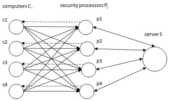
Figure 1. Data transfer system (application).

One solution of the set of all solutions describing optimal capacities $x_j$, $j\in N$ of the data transfer system is vector $x={(2,2,4,5)}^T$.

Assume now that the capacities $x_j$, $j\in N$ are limited by the lower bound ${\underline{x}}_j$ and upper bound ${\overline{x}}_j$. Furthermore, we assume that not all of the processed data have the same importance: whereby, for some more important types of data, all values of the interval must be taken into account (all capacities of the data transfer system have to be involved in optimal solutions), and for some—less important data types—it is sufficient to be considered for at least one value (some value of these capacities of the data transfer system are optimal). In the above defined terminology, the optimal solution has to satisfy the definition of the EA-eigenvector of A.

For numerical illustration of this situation suppose that interval vector X has the form

$$\underline{x}=\left(\begin{array}{c}2\\ 2\\ 3\\ 2\end{array}\right),\overline{x}=\left(\begin{array}{c}4\\ 5\\ 4\\ 3\end{array}\right)$$

with $N^{\exists }=\{1,2\}$, $N^{\forall }=\{3,4\}$ and $N^{\forall }\cup \{n+1\}=\{3,4,5\}$.

Then generators of X and its matrix-vector products can be computed as follows:

$$x^{\left(1\right)}=\left(\begin{array}{c}4\\ 2\\ 0\\ 0\end{array}\right),x^{\left(2\right)}=\left(\begin{array}{c}2\\ 5\\ 0\\ 0\end{array}\right),x^{\left(3\right)}=\left(\begin{array}{c}0\\ 0\\ 4\\ 2\end{array}\right),x^{\left(4\right)}=\left(\begin{array}{c}0\\ 0\\ 3\\ 3\end{array}\right),x^{\left(5\right)}=\left(\begin{array}{c}0\\ 0\\ 3\\ 2\end{array}\right).$$

and

$$A\otimes x^{\left(1\right)}=\left(\begin{array}{c}2\\ 1\\ 2\\ 2\end{array}\right),A\otimes x^{\left(2\right)}=\left(\begin{array}{c}2\\ 1\\ 2\\ 2\end{array}\right),A\otimes x^{\left(3\right)}=\left(\begin{array}{c}2\\ 2\\ 4\\ 2\end{array}\right),$$

$$A\otimes x^{\left(4\right)}=\left(\begin{array}{c}2\\ 2\\ 3\\ 3\end{array}\right),A\otimes x^{\left(5\right)}=\left(\begin{array}{c}2\\ 2\\ 3\\ 2\end{array}\right),$$

By Theorem 2 we will show that X is EA-eigenvector. At first we shall construct matrices C and D and after that we shall solve the system $C\otimes \beta =D\otimes \beta$ with ${\underline{x}}_j\le {\beta }_j\le {\overline{x}}_j$ for $j\in N^{\exists }$ and ${\beta }_i=I$ for $i\in N^{\forall }\cup \{n+1\}$, i.e.,

$$\left(\begin{array}{ccccc}2& 2& 2& 0& 0\\ 1& 1& 2& 0& 0\\ 2& 2& 4& 0& 0\\ 2& 2& 2& 0& 0\\ 2& 2& 0& 2& 0\\ 1& 1& 0& 2& 0\\ 2& 2& 0& 3& 0\\ 2& 2& 0& 3& 0\\ 2& 2& 0& 0& 2\\ 1& 1& 0& 0& 2\\ 2& 2& 0& 0& 3\\ 2& 2& 0& 0& 2\end{array}\right)\otimes \left(\begin{array}{c}{\beta }_1\\ {\beta }_2\\ {\beta }_3\\ {\beta }_4\\ {\beta }_5\end{array}\right)=\left(\begin{array}{ccccc}4& 2& 0& 0& 0\\ 2& 5& 0& 0& 0\\ 0& 0& 4& 0& 0\\ 0& 0& 2& 0& 0\\ 4& 2& 0& 0& 0\\ 2& 5& 0& 0& 0\\ 0& 0& 0& 3& 0\\ 0& 0& 0& 3& 0\\ 4& 2& 0& 0& 0\\ 2& 5& 0& 0& 0\\ 0& 0& 0& 0& 3\\ 0& 0& 0& 0& 2\end{array}\right)\otimes \left(\begin{array}{c}{\beta }_1\\ {\beta }_2\\ {\beta }_3\\ {\beta }_4\\ {\beta }_5\end{array}\right)$$

(3)

with $2\le {\beta }_1\le 4;2\le {\beta }_2\le 5;10\le {\beta }_3\le 10;10\le {\beta }_4\le 10;10\le {\beta }_5\le 10.$

To obtain a solution of the system (3), we use the Algorithm 1 presented in [17]. For the convenience of the reader, the algorithm is described in the original notation.

Let $A,B\in \mathcal{B}(m,n)$ be given matrices. Denote

$$\begin{array}{cc}\hfill \widehat{M}& =\{x\in \mathcal{B}(n);A\otimes x=B\otimes x\},\hfill \\ \hfill I& =\{1,\cdots ,m\},J=\{1,\cdots ,n\},\hfill \\ \hfill a_i\left(x\right)& =\underset{j\in J}{max}(a_{ij}\otimes x_j),b_i\left(x\right)=\underset{j\in J}{max}(b_{ij}\otimes x_j),\hfill \\ \hfill M(\overline{x}& =\{x;x\in \widehat{M}\wedge x\le \overline{x}\},\hfill \\ \hfill I^{<}\left(\overline{x}\right)& =\{i\in I;a_i\left(\overline{x}\right)<b_i\left(\overline{x}\right)\},\hfill \\ \hfill I^{=}\left(\overline{x}\right)& =\{i\in I;a_i\left(\overline{x}\right)=b_i\left(\overline{x}\right)\},\hfill \\ \hfill \alpha \left(\overline{x}\right)& =min\{a_i\left(\overline{x}\right);i\in I^{<}\left(\overline{x}\right)\},\hfill \\ \hfill I^{<}\left(\alpha \left(\overline{x}\right)\right)& =\{i\in I^{<}\left(\overline{x}\right);a_i\left(\overline{x}\right)=\alpha \left(\overline{x}\right)\},\hfill \\ \hfill I^{=}\left(\alpha \left(\overline{x}\right)\right)& =\{i\in I^{=}\left(\overline{x}\right);a_i\left(\overline{x}\right)\le \alpha \left(\overline{x}\right)\},\hfill \\ \hfill J\left(\alpha \left(\overline{x}\right)\right)& =\{j\in J;(\exists i\in I^{<}\left(\alpha \left(\overline{x}\right)\right)[b_{ij}\otimes {\overline{x}}_j>\alpha \left(\overline{x}\right)]\}.\hfill \end{array}$$

Algorithm 1: Solving a general two-sided system.

Input: $m,n,\overline{x}$. Output: $x^{max}$. begin  1  If $\overline{x}\in M\left(\overline{x}\right)$, then $x^{max}:=\overline{x}$, STOP;  2  Change notation so that $a_i\left(\overline{x}\right)\le b_i\left(\overline{x}\right)$ for all $i\in I$;  3  Compute $\alpha \left(\overline{x}\right),I^{<}\left(\alpha \left(\overline{x}\right)\right),I^{=}\left(\alpha \left(\overline{x}\right)\right)$;  4  Set ${\tilde{x}}_j:=\alpha \left(\overline{x}\right)$ if $j\in J\left(\alpha \left(\overline{x}\right)\right),{\tilde{x}}_j:={\overline{x}}_j$ otherwise;  5  If $\tilde{x}\in M\left(\overline{x}\right)$, then $x^{max}:=\tilde{x}$, STOP;  6  Put $\overline{x}:=\tilde{x}$ go to  2 ; end

We will now apply the items of the Algorithm 2 to obtain the greatest solution of the system (3) whereby $\overline{x},a_i\left(\overline{x}\right),b_i\left(\overline{x}\right)$ will be substituted by $\overline{\beta },c_i\left(\overline{\beta }\right),d_i\left(\overline{\beta }\right)$, respectively:

Algorithm 2: Solving a general two-sided system - example.

Input: $m=12,n=5,I=\{1,\cdots ,12\},J=\{1,\cdots ,5\},\overline{x}={(4,5,10,10,10)}^T$. Output: ${\beta }^{max}.$  1 $\overline{\beta }=(4,5,10,10,10)\notin M\left(\overline{\beta }\right)$;  2 $(c_1\left(\overline{\beta }\right),\cdots ,c_{12}\left(\overline{\beta }\right))=(2,2,4,2,2,2,3,3,2,2,3,2)\le$   $(d_1\left(\overline{\beta }\right),\cdots ,d_{12}\left(\overline{\beta }\right))=(4,5,4,2,4,5,3,3,4,5,3,2)$;  3 $\alpha \left(\overline{\beta }\right)=2,I^{<}\left(\alpha \left(\overline{\beta }\right)\right)=I^{<}\left(2\right)=\{1,2,5,6,9,10\},I^{=}\left(\alpha \left(\overline{\beta }\right)\right)=I^{=}\left(2\right)=$   $\{4,12\},J\left(\alpha \left(\overline{\beta }\right)\right)=J\left(2\right)=\{1,2\}$;  4 $\tilde{\beta }=(2,2,10,10,10)$;  5 $\tilde{\beta }=(2,2,10,10,10)\in M\left(\overline{\beta }\right)$, ${\beta }^{max}=\tilde{\beta }$, STOP.

The output of the Algorithm 2 is vector ${\beta }^{max}=(2,2,10,10,10)\in M\left(\overline{\beta }\right)$, which is the greatest possible solution of the system (3). It is easy to verify that the possible solution ${\beta }^{max}$ satisfies all conditions of (3). In other words, ${\beta }^{max}$ is the solution, and we can conclude that X is an EA-eigenvector of A.

4. AE-Eigenvector

As in the previous section, we characterize an interval AE-eigenvector of a given non-interval matrix A with the help of generators. We recall that ${\mathit{X}}_G^{\forall }=\{x^{\left(i\right)},x^{\left[i\right]};i\in N\cup \{n+1\}\}\subseteq {\mathit{X}}^{\forall }$, where

$$x_k^{\left(i\right)}=\left\{\begin{array}{cc}{\overline{x}}_i,\hfill & \mathrm{for}k=i\hfill \\ {\underline{x}}_k,\hfill & \mathrm{otherwise},\hfill \end{array}\right.x_k^{\left[i\right]}=\left\{\begin{array}{cc}{\underline{x}}_i,\hfill & \mathrm{for}k=i\hfill \\ {\overline{x}}_k,\hfill & \mathrm{otherwise},\hfill \end{array}\right.$$

for $i\in N$, and $x^{(n+1)}:={\underline{x}}^{\forall },x^{[n+1]}:={\overline{x}}^{\forall }$.

Theorem 4.

Let $A\in \mathcal{B}(n,n)$ and $\mathit{X}=[\underline{x},\overline{x}]$ be given. Then, X is an AE-eigenvector of A if and only if

$$(\forall x^{\forall }\in {\mathit{X}}_G^{\forall })(\exists x^{\exists }\in {\mathit{X}}^{\exists })A\otimes (x^{\exists }\oplus x^{\forall })=x^{\exists }\oplus x^{\forall }.$$

Proof. 

Suppose that X is not an AE-eigenvector of A; that is,

$$(\exists x^{\forall }\in {\mathit{X}}^{\forall })(\forall x^{\exists }\in {\mathit{X}}^{\exists })A\otimes (x^{\exists }\oplus x^{\forall })\ne (x^{\exists }\oplus x^{\forall })$$

or equivalently

$$(\exists x^{\forall }\in {\mathit{X}}^{\forall })(\forall x^{\exists }\in {\mathit{X}}^{\exists })(\exists i\in N){(A\otimes (x^{\exists }\oplus x^{\forall }))}_i\ne {(x^{\exists }\oplus x^{\forall })}_i.$$

We shall prove that either there is $k\in N\cup \{n+1\}$ such that for each $x^{\exists }\in {\mathit{X}}^{\exists }$ the inequality $A\otimes (x^{\exists }\oplus x^{\left(k\right)})\ne (x^{\exists }\oplus x^{\left(k\right)})$ holds true or there is $k\in N\cup \{n+1\}$ such that for each $x^{\exists }\in {\mathit{X}}^{\exists }$ the inequality $A\otimes (x^{\exists }\oplus x^{\left[k\right]})\ne (x^{\exists }\oplus x^{\left[k\right]})$ is fulfilled.

We will next analyze four cases:

Case (i).

Suppose that $i\in N^{\exists }$ and ${(A\otimes (x^{\exists }\oplus x^{\forall }))}_i<{(x^{\exists }\oplus x^{\forall })}_i.$ We then have

$$\underset{j\in N}{⨁}{a}_{ij}\otimes {(x^{\exists }\oplus x^{\forall })}_j<{(x^{\exists }\oplus x^{\forall })}_i$$

and for ${\underline{x}}^{\forall }=x^{(n+1)}$ we obtain

$$\underset{j\in N}{⨁}{a}_{ij}\otimes {(x^{\exists }\oplus {\underline{x}}^{\forall })}_j\le \underset{j\in N}{⨁}{a}_{ij}\otimes {(x^{\exists }\oplus x^{\forall })}_j<{(x^{\exists }\oplus x^{\forall })}_i=x_i^{\exists }={(x^{\exists }\oplus {\underline{x}}^{\forall })}_i.$$

Case(ii).

Suppose that $i\in N^{\exists }$ and ${(A\otimes (x^{\exists }\oplus x^{\forall }))}_i>{(x^{\exists }\oplus x^{\forall })}_i.$ We then have

$$\underset{j\in N}{⨁}{a}_{ij}\otimes {(x^{\exists }\oplus x^{\forall })}_j=a_{ii}\otimes {(x^{\exists }\oplus x^{\forall })}_i\oplus \underset{j\ne i}{⨁}{a}_{ij}\otimes {(x^{\exists }\oplus x^{\forall })}_j>{(x^{\exists }\oplus x^{\forall })}_i$$

and hence

$$\underset{j\ne i}{⨁}{a}_{ij}\otimes {(x^{\exists }\oplus x^{\forall })}_j>{(x^{\exists }\oplus x^{\forall })}_i$$

because $a_{ii}\otimes {(x^{\exists }\oplus x^{\forall })}_i\le {(x^{\exists }\oplus x^{\forall })}_i$. Moreover, there exists $k\in N,k\ne i$ such that

$$\underset{j\ne i}{⨁}{a}_{ij}\otimes {(x^{\exists }\oplus x^{\forall })}_j=a_{ik}\otimes {(x^{\exists }\oplus x^{\forall })}_k>{(x^{\exists }\oplus x^{\forall })}_i.$$

We will consider two subcases:

Subcase 1: $k\in N^{\forall }$. Then, for $x^{\left(k\right)}$, we obtain

$$\underset{j\in N}{⨁}{a}_{ij}\otimes {(x^{\exists }\oplus x^{\left(k\right)})}_j\ge a_{ik}\otimes {(x^{\exists }\oplus x^{\left(k\right)})}_k=a_{ik}\otimes {(x^{\exists }\oplus {\overline{x}}^{\forall })}_k\ge$$

$$a_{ik}\otimes {(x^{\exists }\oplus x^{\forall })}_k>{(x^{\exists }\oplus x^{\forall })}_i=x_i^{\exists }={(x^{\exists }\oplus x^{\left(k\right)})}_i.$$

Subcase 2: $k\in N^{\exists }$. Then, for $x^{[n+1]}={\overline{x}}^{\forall }$, we obtain

$$\underset{j\in N}{⨁}{a}_{ij}\otimes {(x^{\exists }\oplus {\overline{x}}^{\forall })}_j\ge a_{ik}\otimes {(x^{\exists }\oplus {\overline{x}}^{\forall })}_k\ge$$

$$a_{ik}\otimes {(x^{\exists }\oplus x^{\forall })}_k>{(x^{\exists }\oplus x^{\forall })}_i=x_i^{\exists }={(x^{\exists }\oplus {\overline{x}}^{\forall })}_i.$$

Case (iii).

Suppose that $i\in N^{\forall }$ and ${(A\otimes (x^{\exists }\oplus x^{\forall }))}_i<{(x^{\exists }\oplus x^{\forall })}_i.$ We then have

$$\underset{j\in N}{⨁}{a}_{ij}\otimes {(x^{\exists }\oplus x^{\forall })}_j<{(x^{\exists }\oplus x^{\forall })}_i\iff$$

$$a_{ii}\otimes {(x^{\exists }\oplus x^{\forall })}_i\oplus \underset{j\in N}{⨁}{a}_{ij}\otimes {(x^{\exists }\oplus x^{\forall })}_j<{(x^{\exists }\oplus x^{\forall })}_i$$

and hence it follows that

$$a_{ii}\otimes {(x^{\exists }\oplus x^{\forall })}_i<{(x^{\exists }\oplus x^{\forall })}_i\Rightarrow a_{ii}<{(x^{\exists }\oplus x^{\forall })}_i.$$

Thus, for $x^{\left(i\right)}$ we obtain

$$\underset{j\in N}{⨁}{a}_{ij}\otimes {(x^{\exists }\oplus x^{\left(i\right)})}_j=a_{ii}\otimes {(x^{\exists }\oplus {\overline{x}}^{\forall })}_i\oplus \underset{j\ne i}{⨁}{a}_{ij}\otimes {(x^{\exists }\oplus {\underline{x}}^{\forall })}_j\le$$

$$a_{ii}\otimes {(x^{\exists }\oplus {\overline{x}}^{\forall })}_i\oplus \underset{j\ne i}{⨁}{a}_{ij}\otimes {(x^{\exists }\oplus x^{\forall })}_j<{(x^{\exists }\oplus x^{\forall })}_i=x_i^{\forall }\le {\overline{x}}_i^{\forall }=x_i^{\left(i\right)}={(x^{\exists }\oplus x^{\left(i\right)})}_i.$$

Case (iv).

Suppose that $i\in N^{\forall }$ and ${(A\otimes (x^{\exists }\oplus x^{\forall }))}_i>{(x^{\exists }\oplus x^{\forall })}_i.$ We then have

$$\underset{j\in N}{⨁}{a}_{ij}\otimes {(x^{\exists }\oplus x^{\forall })}_j>{(x^{\exists }\oplus x^{\forall })}_i,$$

hence there is $k\in N,k\ne i$ such that $a_{ik}\otimes {(x^{\exists }\oplus x^{\forall })}_k>{(x^{\exists }\oplus x^{\forall })}_i$ because $a_{ii}\otimes {(x^{\exists }\oplus x^{\forall })}_i\le {(x^{\exists }\oplus x^{\forall })}_i.$

We will consider two subcases:

Subcase 1: $k\in N^{\forall }$. Then, for $x^{\left(k\right)}$, we obtain

$$\underset{j\in N}{⨁}{a}_{ij}\otimes {(x^{\exists }\oplus x^{\left(k\right)})}_j\ge a_{ik}\otimes {(x^{\exists }\oplus x^{\left(k\right)})}_k=a_{ik}\otimes {(x^{\exists }\oplus {\overline{x}}^{\forall })}_k\ge$$

$$a_{ik}\otimes {(x^{\exists }\oplus x^{\forall })}_k>{(x^{\exists }\oplus x^{\forall })}_i=x_i^{\forall }\ge {\underline{x}}_i^{\forall }=x_i^{\left(k\right)}={(x^{\exists }\oplus x^{\left(k\right)})}_i.$$

Subcase 2: $k\in N^{\exists }$. Then, for $x^{\left[i\right]}$, we obtain

$$\underset{j\in N}{⨁}{a}_{ij}\otimes {(x^{\exists }\oplus x^{\left[i\right]})}_j\ge a_{ik}\otimes {(x^{\exists }\oplus x^{\left[i\right]})}_k=a_{ik}\otimes {(x^{\exists }\oplus {\overline{x}}^{\forall })}_k\ge$$

$$a_{ik}\otimes {(x^{\exists }\oplus x^{\forall })}_k>{(x^{\exists }\oplus x^{\forall })}_i=x_i^{\forall }\ge {\underline{x}}_i^{\forall }=x_i^{\left[i\right]}={(x^{\exists }\oplus x^{\left[i\right]})}_i.$$

The reverse implication is trivial. □

The last theorem can be rewritten in the following form:

Corollary 1.

Let $A\in \mathcal{B}(n,n)$ and $\mathit{X}=[\underline{x},\overline{x}]$ be given. Then, X is AE-eigenvector of A if and only if

$$(\forall i\in N\cup \{n+1\})(\exists x{\left(i\right)}^{\exists }\in {\mathit{X}}^{\exists })A\otimes (x{\left(i\right)}^{\exists }\oplus x^{\left(i\right)})=x{\left(i\right)}^{\exists }\oplus x^{\left(i\right)},$$

$$(\forall i\in N\cup \{n+1\}){(\exists x\left[i\right])}^{\exists }\in {\mathit{X}}^{\exists })A\otimes {\left(x\left[i\right]\right)}^{\exists }\oplus x^{\left[i\right]})=x{\left[i\right]}^{\exists }\oplus x^{\left[i\right]}.$$

The next two theorems show that the conditions in Corollary 1 can be equivalently formulated as the solvability conditions of a finite set of two-sided max–min linear systems. Consequently, the interval AE-eigenvectors of a given non-interval matrix can be recognized in polynomial time.

Without loss of generality suppose that $N=N^{\exists }\cup N^{\forall }$, where $N^{\exists }=\{1,2,\cdots ,k\}$ and $N^{\forall }=\{k+1,k+2,\cdots ,n\}$; that is,

$${\mathit{X}}^{\exists }={([{\underline{x}}_1,{\overline{x}}_1],\cdots ,[{\underline{x}}_k,{\overline{x}}_k],[O,O]\cdots ,[O,O])}^T$$

and

$${\mathit{X}}^{\forall }={([[O,O]\cdots ,[O,O],{\underline{x}}_{k+1},{\overline{x}}_{k+1}],\cdots ,[{\underline{x}}_n,{\overline{x}}_n])}^T.$$

Define matrices $C\left(i\right),D\left(i\right),E\left(i\right),F\left(i\right)\in \mathcal{B}(n,k+1)$, for $i\in N^{\forall }\cup \{n+1\}$, as follows

$$\begin{array}{cccc}C\left(i\right)=(A\otimes x^{\left(1\right)}& \cdots & A\otimes x^{\left(k\right)}& A\otimes x^{\left(i\right)})\end{array},\begin{array}{cccc}D\left(i\right)=(x^{\left(1\right)}& \cdots & x^{\left(k\right)}& x^{\left(i\right)})\end{array}$$

$$\begin{array}{cccc}E\left[i\right]=(A\otimes x^{\left(1\right)}& \cdots & A\otimes x^{\left(k\right)}& A\otimes x^{\left[i\right]})\end{array},\begin{array}{cccc}F\left[i\right]=(x^{\left(1\right)}& \cdots & x^{\left(k\right)}& x^{\left[i\right]})\end{array}$$

Also, denote $\beta ={({\beta }_1,\cdots ,{\beta }_k,{\beta }_{k+1})}^T,\gamma ={({\gamma }_1,\cdots ,{\gamma }_k,{\gamma }_{k+1})}^T\in \mathcal{B}(k+1).$

Theorem 5.

Let $A\in \mathcal{B}(n,n)$, $\mathbf{X}$ and $i\in N^{\forall }\cup \{n+1\}$ be given. Then

• $(\exists x^{\exists }\in {\mathit{X}}^{\exists })A\otimes (x^{\exists }\oplus x^{\left(i\right)})=(x^{\exists }\oplus x^{\left(i\right)})$ if and only if the system $C\left(i\right)\otimes \beta =D\left(i\right)\otimes \beta$ with ${\underline{x}}_j\le {\beta }_j\le {\overline{x}}_j$ for $j\in N^{\exists }$ and ${\beta }_{k+1}=I$ is solvable,
• $(\exists x^{\exists }\in {\mathit{X}}^{\exists })A\otimes (x^{\exists }\oplus x^{\left[i\right]})=(x^{\exists }\oplus x^{\left[i\right]})$ if and only if the system $E\left[i\right]\otimes \gamma =F\left[i\right]\otimes \gamma$ with ${\underline{x}}_j\le {\gamma }_j\le {\overline{x}}_j$ for $j\in N^{\exists }$ and ${\gamma }_{k+1}=I$ is solvable.

Proof. 

By Lemma 1, if ${\underline{x}}_j\le {\beta }_j\le {\overline{x}}_j$ for $j\in N^{\exists }$, then $x^{\exists }={\displaystyle \underset{j=1}{\overset{k}{⨁}}}{\beta }_i\otimes x^{\left(j\right)}$ belongs to ${\mathit{X}}^{\exists }$, and if $x^{\exists }\in {\mathit{X}}^{\exists }$ then we can find ${\underline{x}}_j\le {\beta }_j\le {\overline{x}}_j$ for $j\in N^{\exists }$ such that $x^{\exists }={\displaystyle \underset{j=1}{\overset{k}{⨁}}}{\beta }_j\otimes x^{\left(j\right)}$.

We also have the following equivalences for an arbitrary $i\in N^{\forall }\cup \{n+1\}$

$$C\left(i\right)\otimes \beta =D\left(i\right)\otimes \beta \iff$$

$$\underset{j\in N^{\exists }}{⨁}A\otimes x^{\left(j\right)}\otimes {\beta }_j\oplus A\otimes x^{\left(i\right)}\otimes {\beta }_{k+1}=\underset{j\in N^{\exists }}{⨁}{x}^{\left(j\right)}\otimes {\beta }_j\oplus x^{\left(i\right)}\otimes {\beta }_{k+1}\iff$$

$$A\otimes (\underset{j\in N^{\exists }}{⨁}{x}^{\left(j\right)}\otimes {\beta }_j\oplus x^{\left(i\right)})=\underset{j\in N^{\exists }}{⨁}{x}^{\left(j\right)}\otimes {\beta }_j\oplus x^{\left(i\right)}\iff$$

$$(\exists x^{\exists }\in {\mathit{X}}^{\exists })A\otimes (x^{\exists }\oplus x^{\left(i\right)})=x^{\exists }\oplus x^{\left(i\right)}$$

because ${\beta }_{k+1}=I$.

Similarly, we can prove the second part of the theorem. □

Theorem 6.

Suppose that we are given a matrix $A\in \mathcal{B}(n,n)$ and an interval vector $\mathit{X}=[\underline{x},\overline{x}]$. Then, X is an AE-eigenvector of A if and only if for each $i\in N^{\forall }\cup \{n+1\}$ the systems $C\left(i\right)\otimes \beta =D\left(i\right)\otimes \beta$ and $C\left[i\right]\otimes \beta =D\left[i\right]\otimes \beta$ are solvable with ${\underline{x}}_j\le {\beta }_j\le {\overline{x}}_j$ for $j\in N^{\exists }$, ${\beta }_{k+1}=I$ and ${\underline{x}}_j\le {\gamma }_j\le {\overline{x}}_j$ for $j\in N^{\exists }$, ${\gamma }_{k+1}=I$, respectively.

Proof. 

The assertion follows from Theorems 4 and 5. □

Theorem 7.

Suppose that we are given a matrix $A\in \mathcal{B}(n,n)$ and an interval vector $\mathit{X}=[\underline{x},\overline{x}]$. The recognition problem of whether a given interval vector X is an AE-eigenvector of A is then solvable in $O\left(n^4\right)$ time.

Proof. 

According to Theorem 6, the recognition problem of whether a given interval vector X is an AE-eigenvector of A is equivalent to recognizing if the system $C\left(x^{\forall }\right)\otimes \beta =D\left(x^{\forall }\right)\otimes \beta$ is solvable for each $x^{\forall }\in {\mathit{X}}_G^{\forall }$ with ${\underline{x}}_j\le {\beta }_j\le {\overline{x}}_j$ for $j\in N^{\exists }$ and ${\beta }_{k+1}=I$. The computation of a system $A\otimes y=B\otimes y$ needs $O(rs·min(r,s\left)\right)$ time (see [17]), where $A,B\in \mathcal{B}(r,s)$. Therefore, the computation of at most n such systems is done in $n·O\left(n^3\right)=O\left(n^4\right)$ time. □

5. Strong Eigenvectors

In this section, we study various eigenvector types for the interval matrix $\mathit{A}=[\underline{A},\overline{A}]$ and the interval vector $\mathit{X}=[\underline{x},\overline{x}]$. The basic type, which is called a strong eigenvector, is related to all matrices in A and all vectors in X. Further types, which are called strong EA-eigenvectors (strong AE-eigenvectors), are related to all matrices $A\in \mathit{A}$ and to EA-eigenvectors (AE-eigenvectors) derived from X.

Definition 3.

Let $\mathit{A},\mathit{X}$ be given. The interval vector X is called strong eigenvector of A if $(\forall A\in \mathit{A})(\forall x\in \mathit{X})A\otimes x=x.$

Theorem 8.

Let $\mathbf{A},\mathit{X}$ be given. Then, X is a strong eigenvector of A if and only if $\underline{A}\otimes x^{\left(k\right)}=x^{\left(k\right)}$ and $\overline{A}\otimes x^{\left(k\right)}=x^{\left(k\right)}$ for all $k\in N$.

Proof. 

Let us assume that $x\in \mathbf{X}$, $\underline{A}\otimes x^{\left(k\right)}=x^{\left(k\right)}$ and $\overline{A}\otimes x^{\left(k\right)}=x^{\left(k\right)}$ for all $k\in N$. Then, for arbitrary $x\in \mathit{X}$ we get

$$\underline{A}\otimes x=\underline{A}\otimes \underset{i=1}{\overset{n}{⨁}}{\beta }_i\otimes x^{\left(i\right)}=\underset{i=1}{\overset{n}{⨁}}{\beta }_i\otimes (\underline{A}\otimes x^{\left(i\right)})=\underset{i=1}{\overset{n}{⨁}}{\beta }_i\otimes x^{\left(i\right)}=x$$

and

$$\overline{A}\otimes x=\overline{A}\otimes \underset{i=1}{\overset{n}{⨁}}{\beta }_i\otimes x^{\left(i\right)}=\underset{i=1}{\overset{n}{⨁}}{\beta }_i\otimes (\overline{A}\otimes x^{\left(i\right)})=\underset{i=1}{\overset{n}{⨁}}{\beta }_i\otimes x^{\left(i\right)}=x.$$

The assertion follows from the monotonicity of operations; that is, $x=\underline{A}\otimes x\le A\otimes x\le \overline{A}\otimes x=x$ for each $A\in \mathit{A}$. The converse implication is trivial. □

Remark 1.

It is easy to see that the conditions in Theorem 8 can be verified in $O\left(n^3\right)$ time.

Definition 4.

Let $A,X$ be given. Then interval vector X is called

• a strong EA-eigenvector of A if

  $$(\forall A\in \mathit{A})(\exists x^{\exists }\in {\mathit{X}}^{\exists })(\forall x^{\forall }\in {\mathit{X}}^{\forall })A\otimes (x^{\exists }\oplus x^{\forall })=x^{\exists }\oplus x^{\forall },$$
• and a strong AE-eigenvector of A if

  $$(\forall A\in \mathit{A})(\forall x^{\forall }\in {\mathit{X}}^{\forall })(\exists x^{\exists }\in {\mathit{X}}^{\exists })A\otimes (x^{\exists }\oplus x^{\forall })=x^{\exists }\oplus x^{\forall }.$$

Theorem 9.

Let $\mathit{A},\mathit{X}$ be given. The following conditions are equivalent

(i)

X is a strong EA-eigenvector of A,

(ii)

$(\exists x^{\exists }\in {\mathit{X}}^{\exists })(\forall x^{\forall }\in {\mathit{X}}^{\forall })\left[\underline{A}\otimes (x^{\exists }\oplus x^{\forall })=x^{\exists }\oplus x^{\forall }\wedge \overline{A}\otimes (x^{\exists }\oplus x^{\forall })=x^{\exists }\oplus x^{\forall }\right]$,

(iii)

$(\exists x^{\exists }\in {\mathit{X}}^{\exists })(\forall x^{\left(k\right)}\in {\mathit{X}}^{\forall })\left[\underline{A}\otimes (x^{\exists }\oplus x^{\left(k\right)})=x^{\exists }\oplus x^{\left(k\right)}\wedge \overline{A}\otimes (x^{\exists }\oplus x^{\left(k\right)})=x^{\exists }\oplus x^{\left(k\right)}\right]$.

Proof. 

These assertions follow from Theorems 1 and 8. □

Theorem 10.

Let $\mathit{A},\mathit{X}$ be given. The following conditions are equivalent

(i)

X is a strong AE-eigenvector of A,

(ii)

$(\forall x^{\forall }\in {\mathit{X}}^{\forall })(\exists x^{\exists }\in {\mathit{X}}^{\exists })\left[\underline{A}\otimes (x^{\exists }\oplus x^{\forall })=x^{\exists }\oplus x^{\forall }\wedge \overline{A}\otimes (x^{\exists }\oplus x^{\forall })=x^{\exists }\oplus x^{\forall }\right]$,

(iii)

$(\forall x^{\forall }\in {\mathit{X}}_G^{\forall })(\exists x^{\exists }\in X^{\exists })\left[\underline{A}\otimes (x^{\exists }\oplus x^{\forall })=x^{\exists }\oplus x^{\forall }\wedge \overline{A}\otimes (x^{\exists }\oplus x^{\forall })=x^{\exists }\oplus x^{\forall }\right]$.

Proof. 

These assertions follow from Theorems 4 and 8. □

Remark 2.

By Theorems 9 and 10, the verification of whether

(i) 

X is a strong EA-eigenvector,

(ii) 

X is a strong AE-eigenvector,

reduces to finding a vector $x^{\exists }\in {\mathit{X}}^{\exists }$ satisfying some linear max–min equations, similar to Theorems 2 and 6. Hence, the recognition problem for these types of strong eigenvectors is polynomially solvable.

6. EA/AE-Strong Eigenvectors

In the previous sections, we worked with a fixed partition $\mathit{N}=\{N^{\exists },N^{\forall }\}$, with $N=N^{\exists }\cup N^{\forall }$ and $N=N^{\exists }\cap N^{\forall }=\varnothing$. In other words, every index $i\in N$ is associated either with the existential, or with the universal quantifier. According to partition N, the interval vector X is presented as a sum of subintervals ${\mathit{X}}^{\exists }\oplus {\mathit{X}}^{\forall }$. The interpretation of this partition is such that, for technical reasons, the vector entries in subinterval ${\mathit{X}}^{\exists }$ only require the existence of one possible value $x_i\in [{\underline{x}}_i,{\overline{x}}_i]$, while the entries in subinterval ${\mathit{X}}^{\forall }$ require all possible values $x_i\in [{\underline{x}}_i,{\overline{x}}_i]$.

A similar interpretation can be applied to the matrix entries. Suppose that each interval of A is associated either with the universal or with the existential quantifier. We can then split the interval matrix as $\mathit{A}={\mathit{A}}^{\forall }\oplus {\mathit{A}}^{\exists }$, where ${\mathit{A}}^{\forall }$ is the interval matrix comprising universally quantified coefficients and ${\mathit{A}}^{\exists }$ concerns existentially quantified coefficients.

Hence, we work with partition $\tilde{\mathit{N}}=\{{\tilde{N}}^{\exists },{\tilde{N}}^{\forall }\}$, where ${\tilde{N}}^{\exists }\cup {\tilde{N}}^{\forall }=N\times N$ and ${\tilde{N}}^{\exists }\cap {\tilde{N}}^{\forall }=\varnothing$. In other words, ${\underline{a}}_{ij}^{\exists }={\overline{a}}_{ij}^{\exists }=O$ for each pair $(i,j)\in {\tilde{N}}^{\forall }$ and ${\underline{a}}_{ij}^{\forall }={\overline{a}}_{ij}^{\forall }=O$ for each $(i,j)\in {\tilde{N}}^{\exists }.$

Definition 5.

Let A, X be given. Interval vector X is called

• EA-strong eigenvector of A if there is $A^{\exists }\in {\mathit{A}}^{\exists }$ such that for any $A^{\forall }\in {\mathit{A}}^{\forall }$ the vector X is a strong eigenvector of $A^{\exists }\oplus A^{\forall }$,
• AE-strong eigenvector of A if for any $A^{\forall }\in {\mathit{A}}^{\forall }$ there is $A^{\exists }\in {\mathit{A}}^{\exists }$ such that X is a strong eigenvector of $A^{\exists }\oplus A^{\forall }$.

6.1. EA-Strong Eigenvector

Theorem 11.

Let A, X be given. Then, X is an EA-strong eigenvector of A if and only if

$$(\exists A^{\exists }\in {\mathit{A}}^{\exists })(\forall x\in \mathit{X})(A^{\exists }\oplus {\underline{A}}^{\forall })\otimes x=x\wedge (A^{\exists }\oplus {\overline{A}}^{\forall })\otimes x=x.$$

Proof. 

Suppose that there is $A^{\exists }\in {\mathit{A}}^{\exists }$ such that $(A^{\exists }\oplus {\underline{A}}^{\forall })\otimes x=x$ and $(A^{\exists }\oplus {\overline{A}}^{\forall })\otimes x=x$ hold for each $x\in \mathit{X}$. By monotonicity of the operations ⊕ and ⊗ for an arbitrary matrix $A^{\forall }\in {\mathit{A}}^{\forall }$, we get

$$x=(A^{\exists }\oplus {\underline{A}}^{\forall })\otimes x\le (A^{\exists }\oplus A^{\forall })\otimes x\le (A^{\exists }\oplus {\overline{A}}^{\forall })\otimes x=x.$$

The reverse implication trivially holds. □

Theorem 12.

Let A, X be given. Then, X is an EA-strong eigenvector of A if and only if

$$(\exists A^{\exists }\in {\mathit{A}}^{\exists })(\forall i\in N[(A^{\exists }\oplus {\underline{A}}^{\forall })\otimes x^{\left(i\right)}=x^{\left(i\right)}\wedge (A^{\exists }\oplus {\overline{A}}^{\forall })\otimes x^{\left(i\right)}=x^{\left(i\right)}].$$

Proof. 

By Lemma 1, if ${\underline{x}}_j\le {\beta }_j\le {\overline{x}}_j$ for $j\in N$ then $x={\displaystyle \underset{j=1}{\overset{n}{⨁}}}{\beta }_j\otimes x^{\left(j\right)}$ belongs to X; and if $x\in X$, then we can find ${\underline{x}}_j\le {\beta }_j\le {\overline{x}}_j$ for $j\in N$ such that $x={\displaystyle \underset{j=1}{\overset{n}{⨁}}}{\beta }_j\otimes x^{\left(j\right)}$. Then, we have

$$(A^{\exists }\oplus {\underline{A}}^{\forall })\otimes x=(A^{\exists }\oplus {\underline{A}}^{\forall })\otimes \underset{i\in N}{⨁}{\beta }_i\otimes x^{\left(i\right)}=$$

$$\underset{i\in N}{⨁}(A^{\exists }\oplus {\underline{A}}^{\forall })\otimes x^{\left(i\right)}\otimes {\beta }_i=\underset{i\in N}{⨁}{\beta }_i\otimes x^{\left(i\right)}=x.$$

Similarly, we can prove the second equality and by Theorem 11 the assertion follows. The reverse implication trivially holds. □

The last theorem enables us to check the equivalent conditions of Theorem 12 in practice, whereby $(A^{\exists }\oplus {\underline{A}}^{\forall })\otimes x^{\left(i\right)}=x^{\left(i\right)}$ and $(A^{\exists }\oplus {\overline{A}}^{\forall })\otimes x^{\left(i\right)}=x^{\left(i\right)}$ are joined into one system of equalities.

Let A and X be given and ${\tilde{N}}^{\exists }=\{(i_1,j_1),\cdots ,(i_k,j_k)\}$. We denote the block matrix $\tilde{A}\in \mathcal{B}(2n^2,k+1)$ and vectors $\tilde{x}\in \mathcal{B}\left(2n^2\right)$, $\alpha \in \mathcal{B}(k+1)$ as follows

$$\tilde{A}=\left(\begin{array}{ccccccc}{A}^{\left(i_1{j}_1\right)}\otimes x^{\left(1\right)}& \cdots & A^{\left(i_1{j}_k\right)}\otimes x^{\left(1\right)}& A^{\left(i_2{j}_1\right)}\otimes x^{\left(1\right)}& \cdots & A^{\left(i_k{j}_k\right)}\otimes x^{\left(1\right)}& \underline{A}\otimes x^{\left(1\right)}\\ A^{\left(i_1{j}_1\right)}\otimes x^{\left(2\right)}& \cdots & A^{\left(i_1{j}_k\right)}\otimes x^{\left(2\right)}& A^{\left(i_2{j}_1\right)}\otimes x^{\left(2\right)}& \cdots & A^{\left(i_k{j}_k\right)}\otimes x^{\left(2\right)}& \underline{A}\otimes x^{\left(2\right)}\\ ⋮\\ A^{\left(i_1{j}_1\right)}\otimes x^{\left(n\right)}& \cdots & A^{\left(i_1{j}_k\right)}\otimes x^{\left(n\right)}& A^{\left(i_2{j}_1\right)}\otimes x^{\left(n\right)}& \cdots & A^{\left(i_k{j}_k\right)}\otimes x^{\left(n\right)}& \underline{A}\otimes x^{\left(n\right)}\\ A^{\left(i_1{j}_1\right)}\otimes x^{\left(1\right)}& \cdots & A^{\left(i_1{j}_k\right)}\otimes x^{\left(1\right)}& A^{\left(i_2{j}_1\right)}\otimes x^{\left(1\right)}& \cdots & A^{\left(i_k{j}_k\right)}\otimes x^{\left(1\right)}& \overline{A}\otimes x^{\left(1\right)}\\ A^{\left(i_1{j}_1\right)}\otimes x^{\left(2\right)}& \cdots & A^{\left(i_1{j}_k\right)}\otimes x^{\left(2\right)}& A^{\left(i_2{j}_1\right)}\otimes x^{\left(2\right)}& \cdots & A^{\left(i_k{j}_k\right)}\otimes x^{\left(2\right)}& \overline{A}\otimes x^{\left(2\right)}\\ ⋮\\ A^{\left(i_1{j}_1\right)}\otimes x^{\left(n\right)}& \cdots & A^{\left(i_1{j}_k\right)}\otimes x^{\left(n\right)}& A^{\left(i_2{j}_1\right)}\otimes x^{\left(n\right)}& \cdots & A^{\left(i_k{j}_k\right)}\otimes x^{\left(n\right)}& \overline{A}\otimes x^{\left(n\right)}\end{array}\right),$$

$$\tilde{x}={\left(x_1^{\left(1\right)},\cdots ,x_n^{\left(1\right)},\cdots ,x_1^{\left(n\right)},\cdots ,x_n^{\left(n\right)},x_1^{\left(1\right)},\cdots ,x_n^{\left(1\right)},\cdots ,x_1^{\left(n\right)},\cdots ,x_n^{\left(n\right)}\right)}^T,$$

and

$$\alpha ={\left({\alpha }_{11},\cdots ,{\alpha }_{1k},{\alpha }_{21},\cdots ,{\alpha }_{2k},\cdots ,{\alpha }_{k1},\cdots ,{\alpha }_{kk},{\alpha }_{k+1}\right)}^T,$$

where ${\alpha }_{k+1}$ is a variable corresponding to the last column of $\tilde{A}.$

Theorem 13.

Let A, X be given. Then X is EA-strong eigenvector of A if and only if the system $\tilde{A}\otimes \alpha =\tilde{x}$ has a solution α such that ${\underline{a}}_{ij}\le {\alpha }_{ij}\le {\overline{a}}_{ij}$ and ${\alpha }_{k+1}=I.$

Proof. 

The system $\tilde{A}\otimes \alpha =\tilde{x}$ is solvable if and only if there is a vector $\alpha$ such that

$$\underset{i,j=1}{\overset{k}{⨁}}{\alpha }_{ij}\otimes A^{\left(ij\right)}\otimes x^{\left(k\right)}\oplus \underline{A}\otimes x^k=x^{\left(k\right)},$$

$$\underset{i,j=1}{\overset{k}{⨁}}{\alpha }_{ij}\otimes A^{\left(ij\right)}\otimes x^{\left(k\right)}\oplus \overline{A}\otimes x^k=x^{\left(k\right)}$$

for all $k\in N$ with ${\underline{a}}_{ij}\le {\alpha }_{ij}\le {\overline{a}}_{ij}$ and ${\alpha }_{k+1}=I.$ Put $A^{\exists }={\displaystyle \underset{i,j=1}{\overset{k}{⨁}}}{\alpha }_{ij}\otimes A^{\left(ij\right)}$ and by Theorem 12 the assertion holds true. □

Theorem 14.

Suppose that we are given a matrix A and interval vector $\mathit{X}=[\underline{x},\overline{x}]$. The recognition problem of whether a given interval vector X is EA-strong eigenvector of A is solvable in $O\left(n^5\right)$ time.

Proof. 

According to Theorem 13, the recognition problem of whether a given interval vector X is EA-strong eigenvector of A is equivalent to recognizing if the system $\tilde{A}\otimes \alpha =\tilde{x}$ has a solution $\alpha$ with ${\underline{a}}_{ij}\le {\alpha }_{ij}\le {\overline{a}}_{ij}$ and ${\alpha }_{k+1}=I.$ The computation of a system $A\otimes y=b$ needs $O(rs·min(r,s\left)\right)$ time (see [18]), where $A\in \mathcal{B}(r,s),b\in \mathcal{B}\left(r\right)$. Therefore, the computation of such systems is done in $O(n^2·n^2·n)=O\left(n^5\right)$ time. □

6.2. AE-Strong Eigenvector

Denote ${\mathit{A}}_G^{\forall }=\{{\underline{A}}^{\forall },{\overline{A}}^{\forall }\}.$

Theorem 15.

Let A, X be given. Then, X is an AE-strong eigenvector of A if and only if

$$(\forall A^{\forall }\in {\mathit{A}}_G^{\forall })(\exists A^{\exists }\in {\mathit{A}}^{\exists })(\forall x\in \mathit{X})(A^{\exists }\oplus A^{\forall })\otimes x=x.$$

Proof. 

Suppose that for ${\underline{A}}^{\forall }$ there is $B^{\exists }\in {\mathit{A}}^{\exists }$ such that for all $x\in \mathit{X}$ the equality $(B^{\exists }\oplus A^{\forall })\otimes x=x$ holds true and for ${\overline{A}}^{\forall }$ there is $C^{\exists }\in {\mathit{A}}^{\exists }$ such that for all $x\in \mathit{X}$ the equality $(C^{\exists }\oplus A^{\forall })\otimes x=x$ is fulfilled. Moreover, assume that $x\in \mathit{X}$ is arbitrary but fixed. Then, for any $i\in N$ there is $k,l\in N$ such that the following

$${((A^{\forall }\oplus B^{\exists })\otimes x)}_i=\underset{j\in N}{⨁}({\underline{a}}_{ij}^{\forall }\oplus b_{ij}^{\exists })\otimes x_j=({\underline{a}}_{ik}^{\forall }\oplus b_{ik}^{\exists })\otimes x_k\ge ({\overline{a}}_{iv}^{\forall }\oplus c_{iv}^{\exists })\otimes x_v,$$

$$({\underline{a}}_{iv}^{\forall }\oplus b_{iv}^{\exists })\otimes x_v\le ({\overline{a}}_{il}^{\forall }\oplus c_{il}^{\exists })\otimes x_l=\underset{j\in N}{⨁}({\overline{a}}_{ij}^{\forall }\oplus c_{ij}^{\exists })\otimes x_j={((A^{\forall }\oplus C^{\exists })\otimes x)}_i$$

holds for any $v\in N$.

We will prove that for an arbitrary but fixed matrix $A^{\forall }\in {\mathit{A}}^{\forall }$, there is $A^{\exists }\in {\mathit{A}}^{\exists }$ such that $(A^{\exists }\oplus A^{\forall })\otimes x=x.$

Put $A^{\exists }:=B^{\exists }$. Then, there is $r\in N$ such that

$${((B^{\exists }\oplus A^{\forall })\otimes x)}_i=(a_{ir}^{\forall }\oplus b_{ir}^{\exists })\otimes x_r.$$

Consider two cases.

Case 1. For $(i,r)\in {\tilde{N}}^{\forall }$, we get

$$(a_{ir}^{\forall }\oplus b_{ir}^{\exists })\otimes x_r=a_{ir}^{\forall }\otimes x_r\le {\overline{a}}_{ir}^{\forall }\otimes x_r=({\overline{a}}_{ir}^{\forall }\oplus c_{ir}^{\exists })\otimes x_r\le ({\underline{a}}_{ik}^{\forall }\oplus b_{ik}^{\exists })\otimes x_k=x_i.$$

Thus, we have

$${((A^{\forall }\oplus B^{\exists })\otimes x)}_i=(a_{ir}^{\forall }\oplus b_{ir}^{\exists })\otimes x_r\le x_i.$$

The reverse inequality follows from the monotonicity of operations

$$(A^{\forall }\oplus B^{\exists })\otimes x\ge ({\underline{A}}^{\forall }\oplus B^{\exists })\otimes x=x.$$

(4)

Case 2. For $(i,r)\in {\tilde{N}}^{\exists }$, we get

$$(a_{ir}^{\forall }\oplus b_{ir}^{\exists })\otimes x_r=b_{ir}^{\exists }\otimes x_r=({\underline{a}}_{ir}^{\forall }\oplus b_{ir}^{\exists })\otimes x_r\le ({\overline{a}}_{il}^{\forall }\oplus c_{il}^{\exists })\otimes x_l=x_i.$$

Because the reverse inequality trivially follows from (4), the equality ${((B^{\exists }\oplus A^{\forall })\otimes x)}_i=x_i$ is proven.

The reverse implication is trivial. □

Theorem 16.

Let A, X be given. Then, X is AE-strong eigenvector of A if and only if

$$(\forall A^{\forall }\in {\mathit{A}}_G^{\forall })(\exists A^{\exists }\in {\mathit{A}}^{\exists })(\forall k\in N)(A^{\exists }\oplus A^{\forall })\otimes x^{\left(k\right)}=x^{\left(k\right)}.$$

Proof. 

By Lemma 1, if ${\underline{x}}_k\le {\beta }_k\le {\overline{x}}_k$ for $k\in N$, then $x={\displaystyle \underset{k=1}{\overset{n}{⨁}}}{\beta }_k\otimes x^{\left(k\right)}$ belongs to X; and if $x\in \mathit{X}$, then we can find ${\underline{x}}_k\le {\beta }_k\le {\overline{x}}_k$ for $k\in N$ such that $x={\displaystyle \underset{k=1}{\overset{n}{⨁}}}{\beta }_k\otimes x^{\left(k\right)}$. Then, for any $A^{\forall }\in {\mathit{A}}_G^{\forall }$ there is $A^{\exists }\in {\mathit{A}}^{\exists }$ such that for and fixed $x\in \mathit{X}$ we have

$$(A^{\exists }\oplus A^{\forall })\otimes x=(A^{\exists }\oplus A^{\forall })\otimes \underset{k\in N}{⨁}{\beta }_k\otimes x^{\left(k\right)}=$$

$$\underset{i\in N}{⨁}(A^{\exists }\oplus A^{\forall })\otimes x^{\left(k\right)}\otimes {\beta }_k=\underset{k\in N}{⨁}{x}^{\left(k\right)}\otimes {\beta }_k=\underset{k\in N}{⨁}{\beta }_k\otimes x^{\left(k\right)}=x$$

and by Theorem 15 the implication follows. The reverse implication trivially holds true. □

Let A and X be given and ${\tilde{N}}^{\exists }=\{(i_1,j_1),\cdots ,(i_k,j_k)\}$. For each $A^{\forall }\in {\mathit{A}}_G^{\forall }$ and $v\in N$, we denote the block matrix $C(A^{\forall },v)\in \mathcal{B}(n,k+1)$ and $\alpha \in \mathcal{B}(k+1)$ as follows

$$C(A^{\forall },v)=\left(\begin{array}{ccccccc}{A}^{\left(i_1{j}_1\right)}\otimes x^{\left(v\right)}& \cdots & A^{\left(i_1{j}_k\right)}\otimes x^{\left(v\right)}& A^{\left(i_2{j}_1\right)}\otimes x^{\left(v\right)}& \cdots & A^{\left(i_k{j}_k\right)}\otimes x^{\left(v\right)}& A^{\forall }\otimes x^{\left(v\right)}\end{array}\right),$$

and

$$\alpha ={\left({\alpha }_{11},\cdots ,{\alpha }_{1k},{\alpha }_{21},\cdots ,{\alpha }_{2k},\cdots ,{\alpha }_{k1},\cdots ,{\alpha }_{kk},{\alpha }_{k+1}\right)}^T,$$

where ${\alpha }_{k+1}$ is a variable corresponding to the last column of $C(A^{\forall },v).$

Theorem 17.

Let A, X be given. Then, X is an AE-strong eigenvector of A if and only if each $A^{\forall }\in {\mathit{A}}_G^{\forall }$ and for each $v\in N$ the system $C(A^{\forall },v)\otimes \alpha =x^{\left(v\right)}$ has a solution α such that ${\underline{a}}_{ij}\le {\alpha }_{ij}\le {\overline{a}}_{ij}$ and ${\alpha }_{k+1}=I.$

Proof. 

Suppose that $v\in N$ and $A^{\forall }\in {\mathit{A}}_G^{\forall }$ are fixed. The system $C(A^{\forall },v)\otimes \alpha =x^{\left(v\right)}$ is solvable if and only if there is a vector $\alpha$ such that

$$\underset{i,j=1}{\overset{k}{⨁}}{\alpha }_{ij}\otimes A^{\left(ij\right)}\otimes x^{\left(v\right)}\oplus A^{\left(rs\right)}\otimes x^v=x^{\left(v\right)}$$

with ${\underline{a}}_{ij}\le {\alpha }_{ij}\le {\overline{a}}_{ij}$ and ${\alpha }_{k+1}=I.$ Put $A^{\exists }=\underset{i,j=1}{\overset{k}{⨁}}{\alpha }_{ij}\otimes A^{\left(ij\right)}$ and by Theorem 16 the assertion holds true. □

Theorem 18.

Let A, X be given. The recognition problem of whether a given interval vector X is an AE-strong eigenvector of A is solvable in $O\left(n^5\right)$ time.

Proof. 

According to Theorem 17, the recognition problem of whether a given interval vector X is an AE-strong eigenvector of A is equivalent to recognizing if the system $C(A^{\forall },v)\otimes \alpha =x^{\left(v\right)}$ has a solution $\alpha$ with ${\underline{a}}_{ij}\le {\alpha }_{ij}\le {\overline{a}}_{ij}$ and ${\alpha }_{k+1}=I.$ The computation of a system $A\otimes y=b$ needs $O(rs·min(r,s\left)\right)$ time (see [18]), where $A\in \mathcal{B}(r,s),b\in \mathcal{B}\left(r\right)$. Therefore, the computation of such systems is done in $n·O(n·n^2·n)=O\left(n^6\right)$ time. □

7. Conclusions

In this paper, we have presented the properties of steady states in max–min discrete event systems. This concept, in connection with inexact entries and its exists/forall quantification, represents an alternating version to fuzzy discrete events systems which are using vectors and matrices with entries between 0 and 1, and are describing uncertain and vague values. The practical significance of this approach is that some elements of the vector X and the matrix A are taken into account for all values of the interval (corresponding to A-index), and some of them are only considered for at least one value (corresponding to E-index).

The concept of various types of the strong EA/AE-eigenvectors and the EA/AE-strong eigenvectors have been studied. In addition, their characterizations by equivalent conditions are given. All findings have been formally analyzed with a target to estimate the computational complexity of checking the obtained equivalent conditions. The results have been illustrated by an application of the obtained methodology on a numerical example.

The investigation of AE/EA concepts for steady state of discrete events systems with interval data has brought new efficient equivalent conditions. There is a good reason to continue the study of exists/forall quantification method for tolerable, universal and weak eigenvectors which are still unexplored and stay open for future research.

References

- Terano, T.; Tsukamoto, Y. Failure diagnosis by using fuzzy logic. In Proceedings of the IEEE Conference on Decision Control, New Orleans, LA, USA, 7–9 December 1977; pp. 1390–1395. [Google Scholar]
- Zadeh, L.A. Toward a theory of fuzzy systems. In Aspects of Network and Systems Theory; Kalman, R.E., Claris, N.D., Eds.; Hold, Rinehart and Winston: New York, NY, USA, 1971; pp. 209–245. [Google Scholar]
- Sanchez, E. Resolution of eigen fuzzy sets equations. Fuzzy SetsAnd Syst. 1978, 1, 69–74. [Google Scholar] [CrossRef]
- Lin, F.; Ying, H. Fuzzy discrete event systems and their observability. In Proceedings of the Joint 9th IFSA World Congress and 20th NAFIPS International Conference, Vancouver, BC, Canada, 25–28 July 2011; pp. 271–1277. [Google Scholar]
- Lin, F.; Ying, H. Modeling and control of fuzzy discrete event systems. IEEE Trans. Cybern. 2002, 32, 408–415. [Google Scholar]
- Benmessahel, B.; Touahria, M.; Nouioua, F. Predictability of fuzzy discrete event systems. Discret. Event Dyn. Syst. 2017, 27, 641–673. [Google Scholar] [CrossRef]
- Butkovič, P.; Schneider, H.; Sergeev, S. Recognizing weakly stable matrices. SIAM J. Control Optim. 2012, 50, 3029–3051. [Google Scholar] [CrossRef][Green Version]
- Butkovič, P. Max-linear Systems: Theory and Algorithms; Springer Monographs in Mathematics; Springer: Berlin, Germany, 2010. [Google Scholar]
- Fiedler, M.; Nedoma, J.; Ramík, J.; Rohn, J.; Zimmermann, K. Linear Optimization Problems with Inexact Data; Springer: Berlin, Germany, 2006. [Google Scholar]
- Rohn, J. Systems of Linear Interval Equations. Lin. Algebra Appl. 1989, 126, 39–78. [Google Scholar] [CrossRef]
- Molnárová, M.; sková, H.M.; Plavka, J. The robustness of interval fuzzy matrices. Lin. Algebra Appl. 2013, 438, 3350–3364. [Google Scholar] [CrossRef]
- Mysková, H.M.; Plavka, J. XAE and XEA robustness of max–min matrices. Discret. Appl. Math. 2019, 267, 142–150. [Google Scholar] [CrossRef]
- Myšková, H.; Plavka, J. AE and EA robustness of interval circulant matrices in max–min algebra. Fuzzy Sets Syst. 2020, 384, 91–104. [Google Scholar] [CrossRef]
- Plavka, J.; Szabó, P. On the λ-robustness of matrices over fuzzy algebra. Discret. Appl. Math. 2011, 159, 381–388. [Google Scholar] [CrossRef]
- Plavka, J. On the weak robustness of fuzzy matrices. Kybernetika 2013, 49, 128–140. [Google Scholar]
- Plavka, J. On the O(n3) algorithm for checking the strong robustness of interval fuzzy matrices. Discret. Appl. Math. 2012, 160, 640–647. [Google Scholar] [CrossRef]
- Gavalec, M.; Zimmermann, K. Solving systems of two–sided (max,min)–linear equations. Kybernetika 2010, 46, 405–414. [Google Scholar]
- Zimmermann, K. Extremální Algebra; Ekonomicko-matematická laboratoř Ekonomického ústavu ČSAV: Praha, Czech Republic, 1976. [Google Scholar]
© 2020 by the authors. Licensee MDPI, Basel, Switzerland. This article is an open access article distributed under the terms and conditions of the Creative Commons Attribution (CC BY) license (http://creativecommons.org/licenses/by/4.0/).