Market Volatility of the Three Most Powerful Military Countries during Their Intervention in the Syrian War

Abstract

This paper analyzes the volatility dynamics in the financial markets of the (three) most powerful countries from a military perspective, namely, the U.S., Russia, and China, during the period 2015–2018 that corresponds to their intervention in the Syrian war. As far as we know, there is no literature studying this topic during such an important distress period, which has had very serious economic, social, and humanitarian consequences. The Generalized Autoregressive Conditional Heteroscedasticity (GARCH (1, 1)) model yielded the best volatility results for the in-sample period. The weighted historical simulation produced an accurate value at risk (VaR) for a period of one month at the three considered confidence levels. For the out-of-sample period, the Monte Carlo simulation method, based on student t-copula and peaks-over-threshold (POT) extreme value theory (EVT) under the Gaussian kernel and the generalized Pareto (GP) distribution, overstated the risk for the three countries. The comparison of the POT-EVT VaR of the three countries to a portfolio of stock indices pertaining to non-military countries, namely Finland, Sweden, and Ecuador, for the same out-of-sample period, revealed that the intervention in the Syrian war may be one of the pertinent reasons that significantly affected the volatility of the stock markets of the three most powerful military countries. This paper is of great interest for policy makers, central bank leaders, participants involved in these markets, and all practitioners given the economic and financial consequences derived from such dynamics.

1. Introduction

Political uncertainty occurs due to many factors like elections and changes in the government or parliament, changes in policies, strikes, minority disdain, foreign intervention in national affairs, and others. In many cases, these uncertainties lead to further complications affecting the economy and the financial market of the concerned country. Accordingly, the currency could devaluate, prices of assets, commodities, and stocks could fluctuate, and the growth of the economy could be hindered. From this perspective, countries strive to keep political risks controlled to be able to endure the cost or consequence of any sudden political unrest. This is one of the main reasons behind the intervention of powerful countries in the political and military affairs of less powerful countries, which is usually done at a high cost. This paper studies the impact of the intervention of the three most powerful military countries in the world, namely, the United States, Russia, and China (Figure 1), in the Syrian war on their market volatility.

In March 2011, large peaceful protests broke in Syria to call for economic and political reforms with few armed protesters, leading to man arrests. Events evolved into violent acts using artillery and aircrafts, antigovernment rebels, terrorist and extremist attacks, suicide attacks, explosive operations, the intervention of foreign countries, chemical weapons, and others leading to a humanitarian crisis. In 2015, Russia started supporting the Syrian president through financial aid and military support [1]. In the meantime, the United States was providing support for the local Syrians. Later on, the United States and Russia increased their intervention in the war mainly through arms and aircrafts, each supporting their own political interests and allies. By the same token, China’s involvement was shifting from humanitarian assistance and weapon exports [2] to armed forces and increased weapon exports to support its allies’ objectives during this war [3].

Table 1. Countries with the highest military spending worldwide in 2016–2018 (In Billion USD).

In USD Billion	2016	2017	2018
USA	600.1	605.8	648.8
China	216.0	227.8	250.0
Russia	69.2	66.5	61.4
Saudi Arabia	63.7	70.4	67.6
India	56.6	64.6	66.5
France	57.4	60.4	63.8

Source: Stockholm International Peace Research Institute (SIPRI), 2019.

shows countries with the highest military spending in the world for 2016, 2017, and 2018. The U.S. spends the highest budget in the world on defense forces. This expenditure rounded up to USD 649 billion during 2018 based on information from the Stockholm International Peace Research Institute [4]. In fact, the defense spending of the United States alone is higher than the sum of that of the next eight countries in the ranking. These countries include China, Russia, Saudi Arabia, India, France, UK, Japan, and Germany. The country with the second highest defense expenditure is China with USD 250 billion in 2018 compared to USD 228 billion in 2017. As for Russia, its expenditure reached USD 61.4 billion in 2018 compared to USD 66.5 billion in 2017. 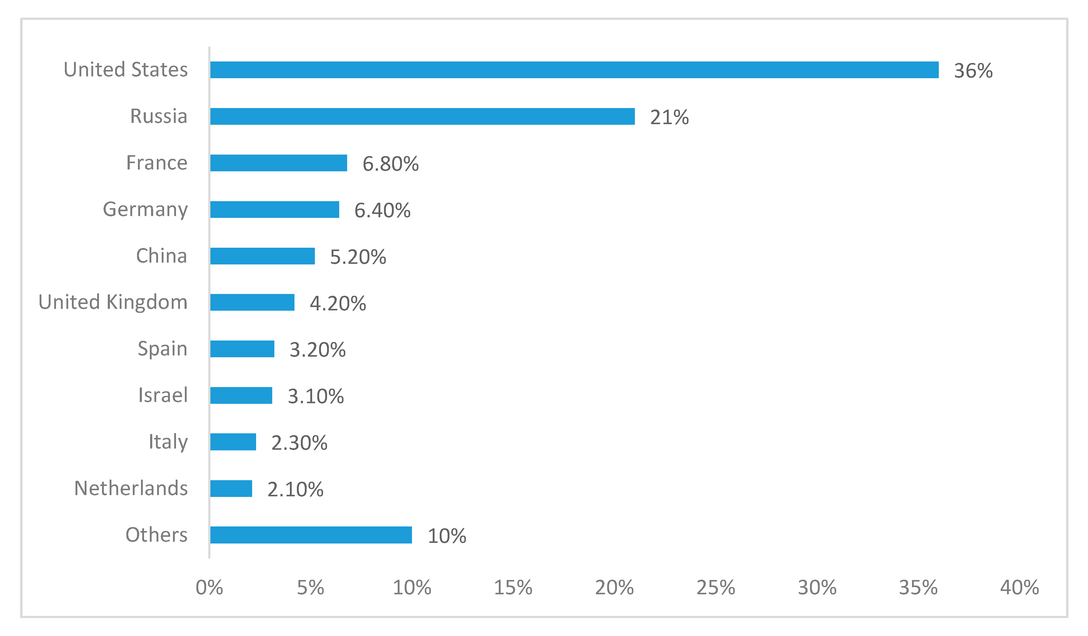Figure 1 represents the 10 largest arms exporters in the world between 2013 and 2017 [5]. Besides having the highest budgets for defense, the U.S. and Russia are also the top exporters of weapons, and China is among the top five worldwide countries. Based on these facts, the importance of the U.S., China, and Russia among military countries is highly reinforced. For this reason, we opted to study the dynamics of their financial markets to comprehend the risks and opportunities they might face, which would affect their worldwide exposure.

To this end, measuring the effect of their intervention in the Syrian war on their financial market volatility is of great importance for policy makers, central bank leaders, analysts, and practitioners because there is a complete absence in the literature of studies that involve the volatility of the financial markets of the U.S., China, and Russia together. Many studies, however, explored the volatility of these countries during different periods and using different volatility models.

In his paper, Wei [6] forecasted the Chinese stock market volatility using non-linear Generalized Autoregressive Conditional Heteroscedasticity (GARCH) models such as the quadratic GARCH (QGARCH) and the Glosten, Jagannathan, and Runkle GARCH (GJR GRACH) models. The author studied seven-year data for the Shanghai Stock Exchange Composite (HSEC) and the Shenzhen Stock Exchange Component (ZSEC). The QGARCH outperformed the linear GARCH model. Furthermore, Lin and Fei [7] concluded that the nonlinear asymmetric power GARCH (APGARCH) model outperformed other GARCH models on different time scales in estimation of the “long memory property of the Shanghai and Shenzhen stock markets”. Recently, Lin [8] studied the volatility of the SSE Composite Index using GARCH models during the period 2013–2017. The asymmetric exponential GARCH (EGARCH (1, 1)) model outperformed the symmetric ones in the forecasting results.

Value at risk (VaR), extreme value theory (EVT), and expected shortfall (ES) models were also used by Wang et al. [9], who implemented an EVT based VaR and ES to estimate the exchange rate risk of the Chinese currency (CNY). They found that the EVT-based VaR estimation produces accurate results for the currency exchange rate risks of EUR/CNY and JPY/CNY. However, EVT underestimated this risk for both exchange rates. Chen et al. [10] estimated VaR and ES by applying EVT on 13 worldwide stock indices. They concluded that China ranks first for VaR and ES with negative returns and ranks third for positive returns with high levels of risk.

A new strategy to estimate daily VaR based on the autoregressive fractionally integrated moving average model (ARFIMA), the multifractal volatility (MFV) model, and EVT was implemented by Wei et al. [11] for the Chinese stock market using high-frequency intraday quotes of the Shanghai Stock Exchange Component (SSEC). This hybrid ARFIMA-MFV-EVT strategy was compared to a number of popular linear and nonlinear GARCH-type-EVT models, i.e., the RiskMetrics, GARCH, IGARCH, and EGARCH models. Although GARCH-type models showed a good performance, VaR results obtained from the ARFIMA-MFV-EVT method outperformed several of them widely used in the literature. Furthermore, Hussain and Li [12] focused on the effect of extreme returns in stock markets on risk management by studying the SSEC index and by using the block maxima (Minima) method (BMM), instead of the popular peaks-over-threshold (POT) method, with various time intervals of extreme daily returns. Three well-known distributions in extreme value theory, i.e., generalized extreme value (GEV), generalized logistic (GL), and generalized Pareto distributions (GP), were employed to model the SSEC index returns. Results showed that GEV and GL distributions are found to be appropriate for the modeling of the extreme upward and downward market movements for China.

Another comparative study, conducted by Hou and Li [13], investigated the transmission of information between the U.S. and China’s index futures markets using an asymmetric dynamic conditional correlation GARCH (DCC GARCH) approach. They found that the correlation between U.S. and Chinese index futures markets increases with the rise of negative shocks in these markets, and that the U.S. index futures market is more efficient in terms of price adjustment, since it is older and more mature. On the other hand, Awartani and Corradi [14] focused on the role of asymmetries in the prediction of the volatility of the S&P 500 Composite Price Index. They examined the relative out-of-sample predictive ability of different GARCH-type models. First, they performed pairwise comparisons of various models against GARCH (1, 1). Then, they carried out a joint comparison of all models. They found that for the case of the one-step ahead pairwise comparison, GARCH (1, 1) is beaten by the asymmetric GARCH models. A similar finding applies to different longer forecast horizons. In the multiple comparison case, GARCH (1, 1) is only beaten when compared against the class of asymmetric GARCH. Another interesting finding is that the RiskMetrics exponential smoothing seems to be the worst model in terms of predictive ability. Furio and Climent [15] studied extreme movements in the return of S&P 500, FTSE 100, and NIKKEI 225 using GARCH-type models and EVT estimates. Results pointed out that more accurate estimates are derived from EVT calculations in both the in-sample and out-of-sample, when compared to less accurate estimates using the GARCH models.

As can be deduced from the review of the above literature, the question of how devastating wars, with indirect consequences all around the world, affect the volatility of financial markets of countries supporting them (and others, of course) might be of core importance for those directly or indirectly involved in such markets. Therefore, the main research question is the following: are the volatility dynamics of those countries affected by an event of the importance of the Syrian war? This paper fills this gap through evaluating the results of a number of traditional volatility models of the GARCH-type family and using EVT and historical simulation (HS) to estimate the VaR of these markets during the Syrian war period.

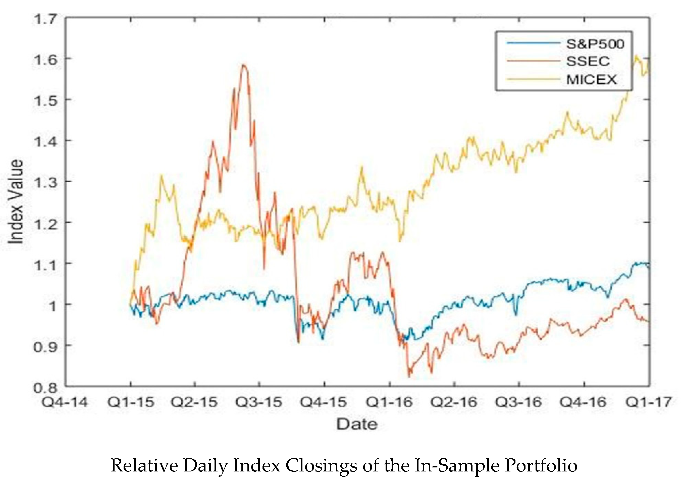
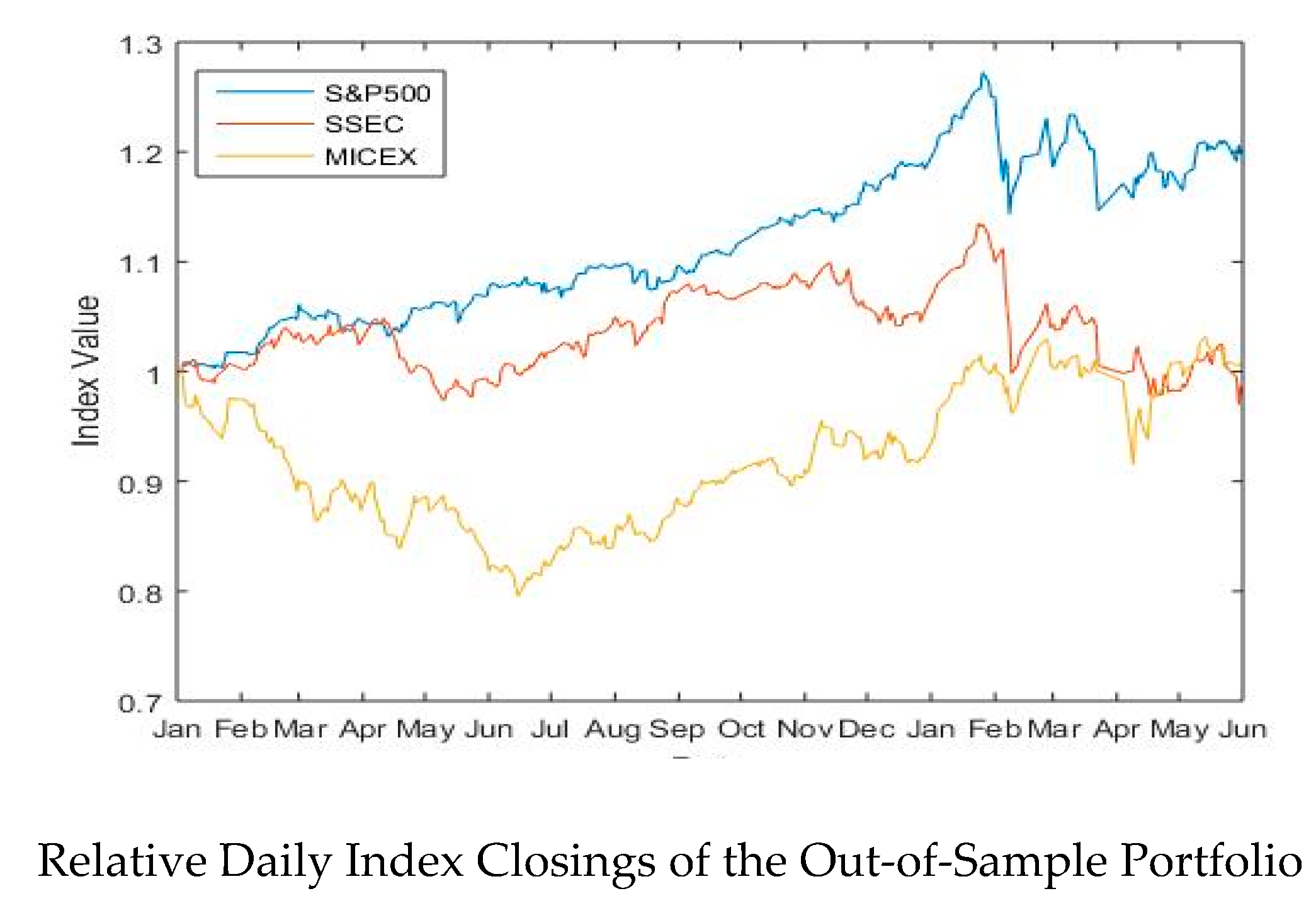
S&P 500 (Standard & Poor’s), SSEC (Shanghai Stock Exchange Composite) and MICEX (Moscow Interbank Currency Exchange) are used to assess the financial markets’ volatility of the U.S., China, and Russia, respectively. The period of study extends from 2015 to 2018. The in-sample period extends from 5 January 2015 until 30 December 2016 as it refers to the beginning of the direct and indirect intervention of the chosen countries in the war in Syria [1]; the out-of-sample interval is 3 January 2017–31 May 2018.

The paper is structured as follows: Section 2 reviews the methodology and the specificities of the applied econometric models, and Section 3 shows the estimated GARCH-type models considered and the selection process. This section also depicts the results related to the calculation of VaR using HS volatility and the “peaks-over-threshold” (POT) EVT model under the GP distribution. Section 4 concludes and discusses the empirical findings.

2. Econometric Models

As previously outlined, we use the GARCH (1, 1) and EGARCH (1, 1) as competing models to measure the volatility of the financial markets of the U.S., Russia, and China. GARCH models are commonly used by financial institutions to obtain volatility and correlation forecasts of asset and risk factor return. We use the symmetric normal GARCH given its strength to provide short- and medium-term volatility forecasts. We also use EGARCH, the asymmetric GARCH model, which is widely recognized in providing a better in-sample fit than other types of GARCH processes and avoids the need for any parameter constraints (see [16,17] for details on other GARCH-type models). The exponentially weighted moving average (EWMA) model is not used because it does not account for mean reversion and overvalue volatility after severe price fluctuation [18]. As said in the introductory section, for VaR estimation with high confidence intervals, we apply EVT [19], and more specifically GEV, GL, and GP distributions. We decided to use EVT because of its ability to provide good estimates and serve of help in situations where high confidence levels are needed, since EVT has proven to be a robust way of smoothing and extrapolating the tails of an empirical distribution [20]. The EVT implementation in this paper is based on a multivariate analysis to accurately measure the VaR of the portfolio composed of the U.S., Russia, and China stock markets. We also estimate the VaR of the portfolio using HS for comparison.

2.1. GARCH Model

The pioneering work of Engle [21], where the Autoregressive Conditional Heteroscedasticity (ARCH) model (that relates the current level of volatility to p past squared error terms) was introduced, constitutes the main pillar of modern financial econometrics. However, the ARCH strategy has some limitations, including the typically required 5–8 lagged error terms to adequately model conditional variance. That was the reason for this model to be generalized by Bollerslev [22], giving rise to the generalized ARCH (GARCH) model, by adding lagged conditional variance, which acts as a smoothing term. In practical terms, the GARCH (p, q) model builds on the ARCH (p) by including q lags of the conditional variance. Therefore, a GARCH specification uses the weighted average of long-run variance, the predicted variance for the current period, and any new information in this period, as captured by the squared residuals, to forecast a future variance. More specifically, the general GARCH (p, q) model is as shown in Equation (1):

$${\sigma }_t^2=\gamma V_L+{\displaystyle \sum _{i=1}^p{\alpha }_i{u}_{t-i}^2}+{\displaystyle \sum _{j=1}^q{\beta }_j{\sigma }_{t-j}^2}$$

(1)

where ${\sigma }_t^2$ is the time t − 1 conditional variance, $V_L$ is the long run average variance, ${\sigma }_{t-j}^2$ are the lags of the conditional variance, and $u_{t-i}^2$ are the lagged squared error terms. $u_t={\sigma }_t{e}_t$ with $e_t$ i.i.d. N(0, 1). Coefficients $\gamma$, ${\alpha }_i$ and ${\beta }_j$ are the weights for $V_L$ and the lags of the conditional variance and the squared error terms, respectively, and their estimates are obtained by Maximum Likelihood.

GARCH (1, 1) is the most used model of all GARCH models. It can be written as follows:

$${\sigma }_t^2=\gamma V_L+{\alpha }_1{u}_{t-1}^2+{\beta }_1{\sigma }_{t-1}^2$$

(2)

or, alternatively,

$${\sigma }_t^2=\omega +{\alpha }_1{u}_{t-1}^2+{\beta }_1{\sigma }_{t-1}^2$$

(3)

where $\omega =\gamma V_L.$ Coefficients in the GARCH specification sum up to the unity and have to be restricted for the conditional variances to be uniformly positive. In the case of the GARCH (1, 1) such restrictions are: $\omega >0$, ${\alpha }_1\ge 0$ and ${\beta }_1\ge 0$. In addition, the requirement for stationarity is $1-{\alpha }_1-{\beta }_1>0$. The unconditional variance can be shown to be $E\left({\sigma }_t^2\right)=\omega /\left(1-{\alpha }_1-{\beta }_1\right)$.

2.2. EGARCH Model

The EGARCH model was proposed by Nelson [23] to capture the leverage effects observed in financial series and represents a major shift from the ARCH and GARCH models. The EGARCH specification does not model the variance directly, but its natural logarithm. This way, there is no need to impose sign restrictions on the model parameters to guarantee that the conditional variance is positive. In addition, EGARCH is an asymmetric model in the sense that the conditional variance depends not only on the magnitude of the lagged innovations but also on their sign. This is how the model accounts for the different response of volatility to the upwards and downwards movement of the series of the same magnitude. More specifically, EGARCH implements a function $g\left(e_t\right)$ of the innovations $e_t$, which are i.i.d. variables with zero mean, so that the innovation values are captured by the expression $\left|e_t\right|-E\left|e_t\right|$.

An EGARCH (p, q) is defined as:

$$\log {\sigma }_t^2=\omega +{\displaystyle \sum _{j=1}^q{\beta }_j\log {\sigma }_{t-j}^2}+{\displaystyle \sum _{j=1}^p{\theta }_{i}g\left(e_{t-j}\right)}$$

(4)

where $g\left(e_t\right)=\delta e_t+\alpha \left(\left|e_t\right|-E\left|e_t\right|\right)$ are variables i.i.d. with zero mean and constant variance. It is through this function that depends on both the sign and magnitude of $e_t$, that the EGARCH model captures the asymmetric response of the volatility to innovations of different sign, thus allowing the modeling of a stylized fact of the financial series: negative returns provoke a greater increase in volatility than positive returns do.

The innovation (standardized error divided by the conditional standard deviation) is normally used in this formulation. In such a case, $E\left|e\right|=\sqrt{2/\pi }$ and the sequence $g\left(e_t\right)$ is time independent with zero mean and constant variance, if finite. In the case of Gaussianity, the equation for the variance in the model EGARCH (1, 1) is:

$$\log {\sigma }_t^2=\omega +\beta \log {\sigma }_{t-1}^2+\delta e_{t-1}+\alpha \left(\left|e_{t-1}\right|-\sqrt{\frac{2}{\pi }}\right).$$

(5)

Stationarity requires $\left|\beta \right|<1$, the persistence in volatility is indicated by $\beta$, and $\delta$ indicates the magnitude of the leverage effect. $\delta$ is expected to be negative, which implies that negative innovations have a greater effect on volatility than positive innovations of the same magnitude. As in the case of the standard GARCH specification, maximum likelihood is used for the estimation of the model.

2.3. EVT

EVT deals with the stochastic behavior of extreme events found in the tails of probability distributions, and, in practice, it has two approaches. The first one relies on deriving block maxima (minima) series as a preliminary step and is linked to the GEV distribution. The second, referred to as the peaks over threshold (POT) approach, relies on extracting, from a continuous record, the peak values reached for any period during which values exceed a certain threshold and is linked to the GP distribution [24]. The latter is the approach used in this paper.

The generalized Pareto distribution was developed as a distribution that can model tails of a wide variety of distributions. It is based on the POT method which consists in the modelling of the extreme values that exceed a particular threshold. Obviously, in such a framework there are some important decisions to take: (i) the threshold, μ; (ii) the cumulative function that best fits the exceedances over the threshold; and (iii) the survival function, that is, the complementary of the cumulative function.

The choice of the threshold implies a trade-off bias-variance. A low threshold means more observations, which probably diminishes the fitting variance but probably increases the fitting bias, because observations that do not belong to the tail could be included. On the other hand, a high threshold means a fewer number of observations and, maybe, an increment in the fitting variance and a decrement in the fitting bias.

As for the distribution function that best fits the exceedances over the threshold, let us suppose that $F(x)$ is the distribution function for a random variable $X$, and that threshold $\mu$ is a value of $X$ in the right tail of the distribution; let y denote the value of the exceedance over the threshold $\mu$. Therefore, the probability that X lies between $\mu$ and $\mu +y \left(y>0\right)$ is $F(\mu +y)-F(\mu )$ and the probability for X greater than $\mu$ is $1-F(\mu )$. Writing the exceedances (over a threshold $\mu$) distribution function $F^{\mu }(y)$ as the probability that X lies between $\mu$ and $\mu +y$ conditional on $X>\mu$, and taking into account the identity linking the extreme and the exceedance: $X=Y+\mu$, it follows that:

$$F^{\mu }(y)=P\left(Y\le y|X>\mu \right)=P\left(\mu <X\le \mu +y|X>\mu \right)=\frac{F(x)-F(\mu )}{1-F(\mu )}$$

(6)

and that

$$1-F^{\mu }(y)=1-\frac{F(x)-F(\mu )}{1-F(\mu )}=\frac{1-F(x)}{1-F(\mu )}$$

(7)

In the case that the parent distribution F is known, the distribution of threshold exceedances also would be known. However, this is not the practical situation, and approximations that are broadly applicable for high values of the threshold are sough. Here is where Pickands–Balkema–de Haan theorem ([25,26]) comes into play. Once the threshold has been estimated, the conditional distribution $F^{\mu }(y)$ converges to the GP distribution. It is known that $F^{\mu }(y)\to G_{\xi ,\sigma }\left(y\right)$ as $\mu \to \infty$, with

$$G_{\xi ,\sigma }\left(y\right)=\{\begin{array}{ll}1-{\left(1+\xi \frac{y}{\sigma }\right)}^{-\frac{1}{\xi }}& \mathrm{if} \xi \ne 0 \\ 1-e^{-\frac{y}{\sigma }}& \mathrm{if} \xi =0 \end{array}$$

(8)

where $\sigma >0$ and $y\ge 0$ if $\xi \ge 0$ and $0\le y\le -\sigma /\xi$ if $\xi <0$. $\xi$ is a shape parameter that determines the heaviness of the tail of the distribution, and σ is a scale parameter. When $\xi =0$, $G_{\xi ,\sigma }\left(y\right)$ reduces to the exponential distribution with expectation $\exp \left(\sigma \right)$; in the case that $\xi <0$, it becomes a Uniform $\left(0,\sigma \right)$; finally, $\xi >0$ leads to the Pareto distribution of the second kind [27]. In general, $\xi$ has a positive value between 0.1 and 0.4. The GP distribution parameters are estimated via maximum likelihood.

Once the maximum likelihood estimates are available, a specific GP distribution function is selected, and an analytical expression for VaR with a confidence level q can be defined as a function of the GP distribution parameters:

$$Va{R}_{\widehat{q}}=\mu +\frac{\widehat{\sigma }\left(\mu \right)}{\widehat{\xi }}\left(\frac{N}{N_{\mu }}{\left(1-q\right)}^{-\widehat{\xi }}-1\right)$$

(9)

where N is the number of observations in the left tail and $N_{\mu }$ is the number of excesses beyond the threshold $\mu$.

$$Va{R}_{\widehat{q}}=\mu +\frac{\widehat{\sigma }\left(\mu \right)}{\widehat{\xi }}\left(\frac{N}{N_{\mu }}{\left(1-q\right)}^{-\widehat{\xi }}-1\right)$$

(10)

3. Results

3.1. Descriptive Statistics

Data for 3 years were extracted from the Bloomberg platform for the three selected stock market indices and were manipulated to derive the return from the closing prices corresponding to each index. For the in-sample period, 458 daily observations were studied compared to 315 for the out-of-sample forecast period. It is important to note that in November 2017, the name of the MICEX index (composed of Russian stocks of the top 50 largest issues in the Moscow Exchange) was officially changed to the MOEX Russia Index, representing the “Russian stock market benchmark” [28].

Table 2. Descriptive Statistics of S&P 500, SSEC, and MICEX: 5 January 2015–30 December 2016 and 3 January 2017–31 May 2018.

Stock Markets	S&P 500 (In-Sample)	SSEC (In-Sample)	MICEX (In-Sample)	S&P 500 (Out-of-Sample)	SSEC (Out-of-Sample)	MICEX (Out-of-Sample)
Mean	0.022%	−0.017%	0.017%	0.060%	−0.001%	0.054%
Standard Deviation	1.0%	2.10%	1.2%	0.711%	0.774%	1.025%
Skewness	1.0%	2.10%	1.2%	0.711%	0.774%	1.025%
Kurtosis	3.33	4.62	0.97	7.93	4.83	12.45
Median	0.01%	0.10%	0.04%	0.06%	0.08%	−0.05%
Minimum	−4.0%	−10.8%	−4.4%	−4.18%	−4.14%	−8.03%
Maximum	4.7%	6.0%	4.4%	2.76%	2.15%	3.89%
1st Quartile	−0.41%	−0.66%	−0.65%	−0.18%	−0.35%	−0.51%
3rd Quartile	0.49%	0.87%	0.85%	0.34%	0.40%	0.54%

lists the descriptive statistics of S&P 500, SSEC, and MICEX for the in- and out-of-sample periods. Surprisingly, S&P 500 and the MICEX behaved similarly in terms of return during the in-sample and out-of-sample periods.

In reference to the two chosen time periods, the skewness of the returns of the three indices is close to 0 and the returns display excess in kurtosis. This implies that the distributions of returns are not normal as confirmed by Jarque-Bera normality tests (

Table 3. Jarque-Bera Normality Test of S&P 500, SSEC, and MICEX.

Stock Markets	In-Sample		Out-of-Sample
	Score	p-Value	Score	p-Value
S&P 500	198.66	0.000	865.78	0.000
SSEC	483.75	0.000	352.63	0.000
MICEX	18.12	0.000	2027.03	0.000

Note: p-value refers to Jarque–Bera normality test, Ho: the index return is normally distributed.

). The distributions of returns are stationary according to the augmented Dicky–Fuller (ADF) test applied to the three indices (

Table 4. ADF Stationarity Test.

	Critical Values at 5%	STAT	p-Value	STAT	p-Value	STAT	p-Value
		S&P 500		SSEC		MICEX
No Constant	−1.9	−28.4	0.001	−12.8	0.001	−26.9	0.001
Constant Only	−2.9	−28.4	0.001	−12.8	0.001	−11.6	0.001
Constant and Trend	−1.6	−28.4	0.000	−12.7	0.000	−11.6	0.000
Constant, Trend, and Trend2	−1.6	−28.4	0.000	−12.7	0.000	−11.6	0.000

Note: ADF p-value refers to the augmented Dickey–Fuller unit root test, Ho: the index return has a unit root.

).

3.2. GARCH (1, 1) and EGARCH (1, 1) Results

GARCH (1, 1) and EGARCH (1, 1) parameters were estimated using the daily returns of each index. Results from the normal distribution, the student’s t-distribution and the Generalized Error Distribution (GED) were derived. The goodness of fit test and residual analysis were then performed to ensure that the assumptions of the applied models were all met. The model parameters were estimated by maximum likelihood.

Table 5. Estimates of the Parameters of GARCH (1,1) and EGARCH (1,1) (with GED).

	S&P 500	SSEC	MICEX
		GARCH (1, 1)
Long-run mean (µ)	0.000249	−0.00009	0.00080
Omega (ω)	8.5218 × 10−6	1.1035 × 10−6	2.9655 × 10−6
ARCH component (α)	0.1972	0.0569	0.0653
GARCH component (β)	0.7105	0.9331	0.9065
		EGARCH (1, 1)
Long-run mean (µ)	0.00030	−0.00009	0.00142
Omega (ω)	−0.72879	−0.08598	−0.87318
ARCH component (α)	0.04766	0.20530	0.30477
Leverage coefficient ($\delta$)	−0.29149	−0.01362	0.05345
GARCH component (β)	0.92471	0.98689	0.90237

Note: The GED was selected after checking the average, standard deviation, skewness, kurtosis, the noise, and ARCH tests corresponding to the three distributions.

presents a summary of such estimates for GARCH (1, 1) and EGARCH (1,1).

3.3. Best Volatility Model Selection for the In- and Out-of-Sample Periods

The root mean square error (RMSE), the mean absolute error (MAE), and the mean absolute percentage error (MAPE) are implemented to choose the best volatility model. For S&P 500, we compared the estimated volatility to the implied volatility. However, this was not possible for SSEC and MICEX due the absence of data. Results depicted in

Table 6. In-Sample Period Error Statistics.

S&P 500 during In-Sample Period (from 5 January 2015 till 30 December 2016)
	RMSE	Rating	MAE	Rating	MAPE	Rating
Implied Vol.	0.047694	2	0.039028	2	0.00377	3
GARCH (1, 1)	0.040995	1	0.028954	1	0.002376	1
EGARCH (1, 1)	0.049947	3	0.039066	3	0.003261	2
SSEC during In-Sample Period (from 5 January 2015 till 30 December 2016)
GARCH (1, 1)	0.09567	1	0.080424	1	0.002879	1
EGARCH (1, 1)	0.11588	2	0.090075	2	0.003134	2
MICEX during In-Sample Period (from 5 January 2015 till 30 December 2016)
GARCH (1, 1)	0.184631	1	0.173261	1	0.004775	1
EGARCH (1, 1)	0.188566	2	0.179723	2	0.004997	2
S&P 500 during Out-of-Sample (from 3 January 2017 till 31 May 2018)
Implied Vol.	0.04809	3	0.04325	3	0.006092	3
GARCH (1, 1)	0.040024	1	0.035135	1	0.004896	1
EGARCH (1, 1)	0.047078	2	0.041034	2	0.005689	2
SSEC during Out-of-Sample (from 3 January 2017 till 31 May 2018)
GARCH (1, 1)	0.08478	2	0.080437	2	0.004033	2
EGARCH (1, 1)	0.07113	1	0.063535	1	0.00322	1
MICEX during Out-of-Sample (from 3 January 2017 till 31 May 2018)
GARCH (1, 1)	0.071894	2	0.064616	2	0.002909	2
EGARCH (1, 1)	0.069381	1	0.061135	1	0.00271	1

Note: $RME=\sqrt{{\displaystyle \sum _{t=1}^n{\left(f-Y\right)}^2}/n}$; $MAE={\displaystyle \sum _{t=1}^n\left|f-Y\right|}/n$; $MAPE=100{\displaystyle \sum _{t=1}^n\left|\frac{f-Y}{Y}\right|}/n$, where n is the number of periods, Y is the true value and f is the prediction value. The best model is the one that has a minimum value of RMSE, MAE and MAPE.

reveal the superiority of GARCH (1, 1) in estimating the volatility of the three countries in the in-sample period, which coincides with the peak period of the Syrian war. As for the out-of-sample period, while GARCH (1, 1) ranks first for S&P 500, EGARCH (1, 1) ranks first for the SSEC and MICEX with a difference in RMSE of around 0.002 and 0.01 units respectively as compared to GARCH (1, 1). Volatilities estimated with the superior volatility models in comparison to the realized volatilities for the out-of-sample period are depicted in Figure 2.

3.4. VaR Output

Based on the superior model corresponding to each index, a portfolio of volatility updates was established for each sample period. First, the historical simulation approach was implemented. It involved incorporating volatility in updating the historical return. Because the volatility of a market variable may vary over time, we modified the historical data to reflect the variation in volatility. This approach uses the variation in volatility in a spontaneous way to estimate VaR by including more recent information. Second, a Monte Carlo simulation method including student t-copula and EVT was applied to the created portfolio composed of the three markets to estimate VaR with different confidence levels. The filtered residuals of each return series were extracted using EGARCH. The Gaussian kernel estimate was used for the interior marginal cumulative distribution function (CDF) and the generalized Pareto distribution (GP) was applied to estimate the upper and lower tails. The student t-copula was also applied to the portfolio’s data in order to reveal the correlation among the residuals of each index. This process led to the estimation of the portfolio’s VaR over a horizon of one month and confidence levels of 90%, 95%, and 99%.

Table 7. VaR Summary Results.

Outcome	HS (Volatility Weighted)	EVT	Real VaR
In-Sample
90% VaR	0.68%	2.93%	1.31%
95% VaR	1.03%	4.83%	1.68%
99% VaR	2.31%	8.39%	2.38%
Out-of-Sample
90% VaR	0.48%	3.76%	0.73%
95% VaR	0.71%	5.47%	0.94%
99% VaR	1.65%	9.60%	1.33%

summarizes all the VaR estimates calculated for the in-sample and out-of-sample periods using HS and EVT compared to the Real VaR. The visual illustrations of the relevant outcomes related to the logarithmic returns of the selected stock indices, the auto-correlation function (ACF) of returns and of the squared returns, the filtered residuals and the filtered conditional standard deviation, the ACF of standardized residuals, and the upper tail of standardized residuals for both periods, are presented in Appendix A (Figure A1 and Figure A2).

It is apparent that VaR with a confidence level of 99%, using HS and EVT, overrates the risk for the three countries during both periods. Furthermore, the HS VaR results are closer to the Real VaR results compared to those of the EVT VaR. This is not altogether surprising since the EVT method is concerned with studying the behavior of extremes within these markets rather than simply fitting the curve. Therefore, the above output represents a benchmark that can be extrapolated beyond the data during stress periods.

4. Discussion

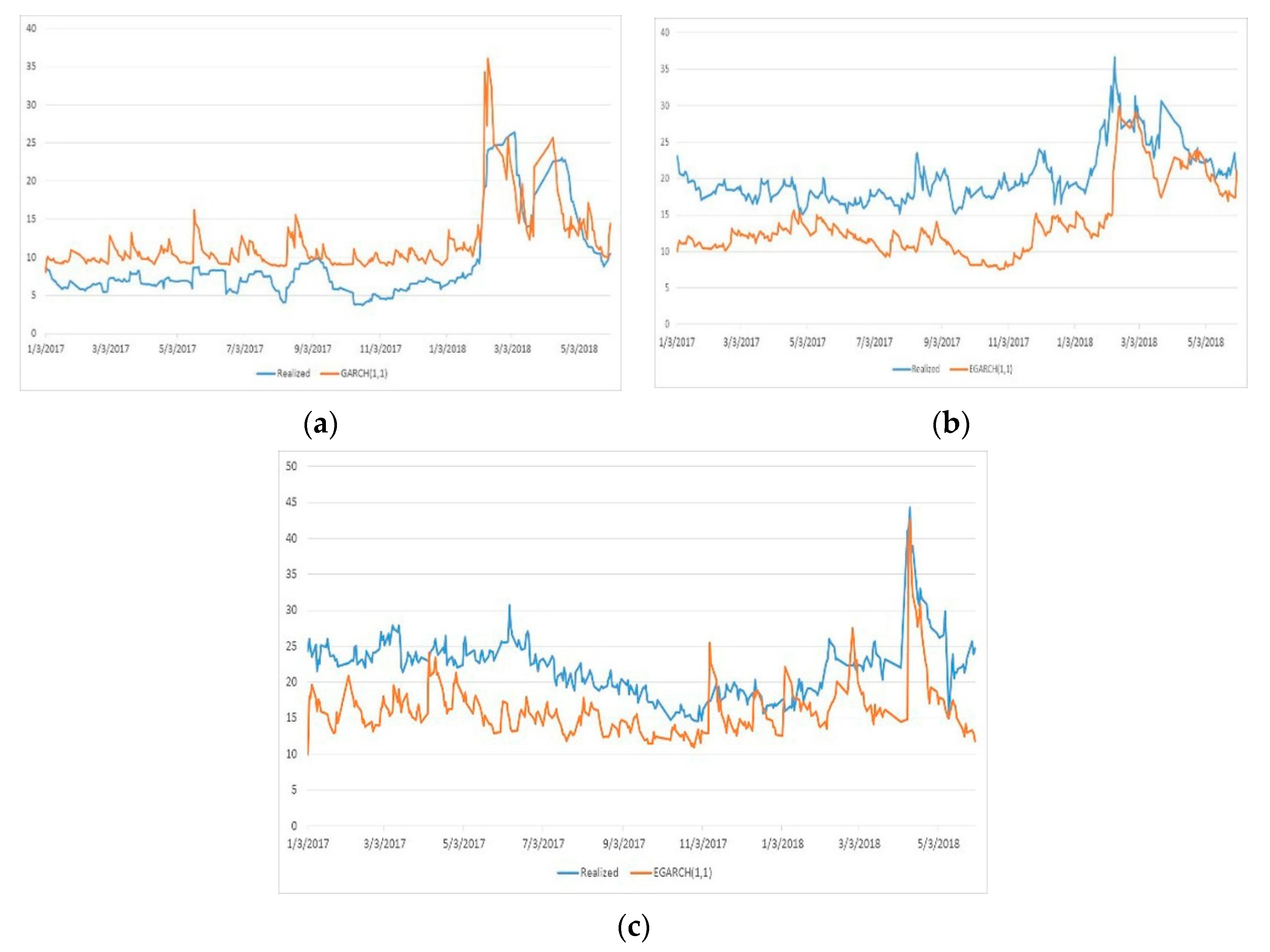
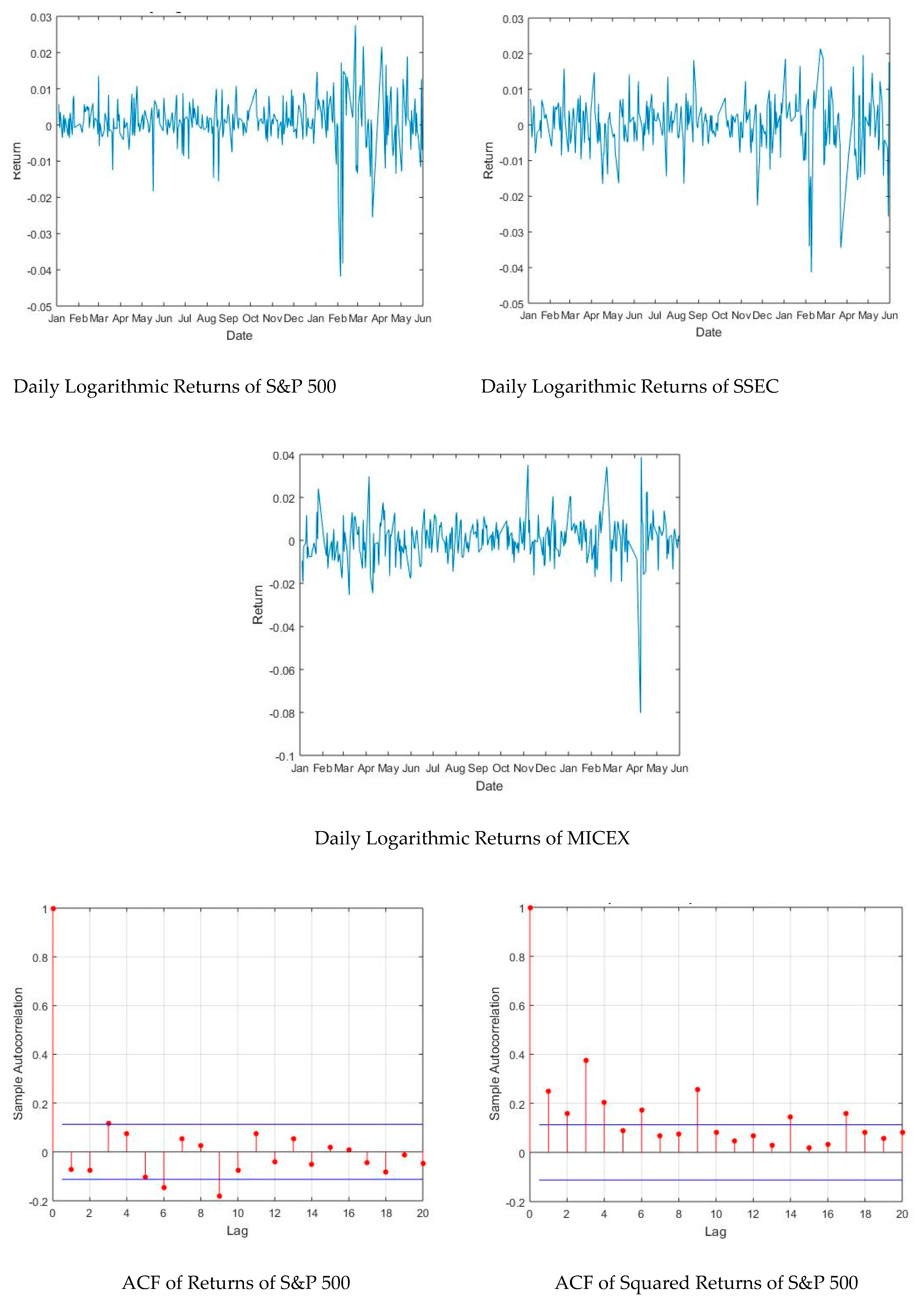
This paper revealed original common points among the most powerful military countries in the world regarding the behavior of their financial markets during the period 2015–2018, which corresponds to their intervention in the Syrian war. First, the returns of S&P 500 and MICEX were quite similar during the in-sample and out-of-sample periods. Second, the GARCH (1, 1) was found to be the best volatility model for the in-sample period for S&P 500, MICEX, and SSEC, outperforming EGARCH (1, 1). The incorporation of the GARCH (1, 1) specification to the HS produced an accurate VaR for a period of one month, at the three confidence levels, compared to the real VaR.

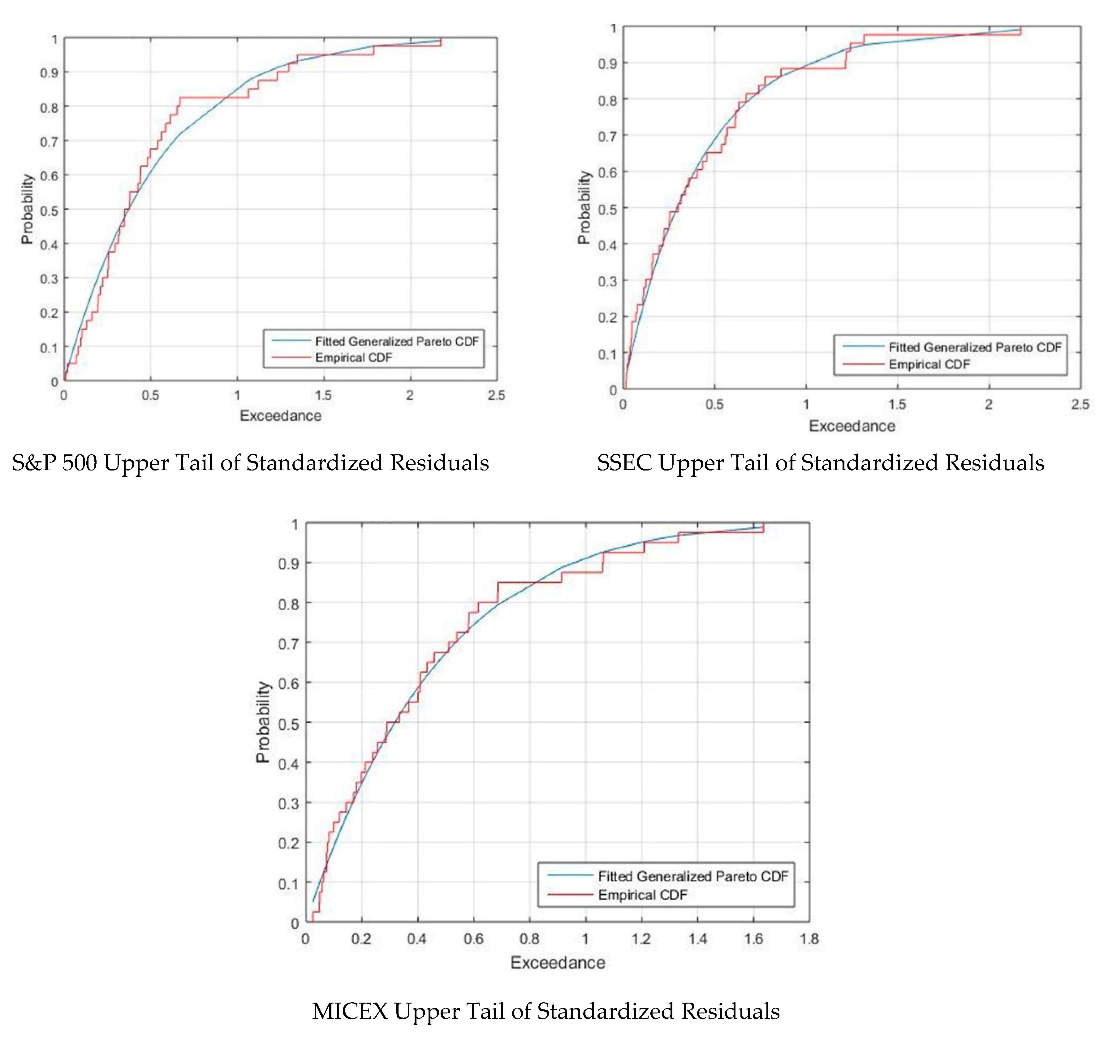
EVT VaR results are consistent with those found by Furio and Climent [15] and Wang et al. [9], who highlighted the accuracy of studying the tails of loss severity distribution of several stock markets. Furthermore, part of our results corroborates the work of Peng et al. [29], who showed that EVT GP distribution is superior to certain GARCH models implemented on the Shanghai Stock Exchange Index.

The GP distribution highlighted the behavior of “extremes” for the U.S., Russian, and Chinese financial markets, which is of great importance since it emphasizes the risks and opportunities inherent to the dynamics of their markets and also underlines the uncertainty corresponding to their worldwide exposure.

Expected EVT VaR values of 3.76%, 5.47%, and 9.60%, at 90%, 95%, and 99% confidence levels, respectively (for the out-of-sample period), might appear overstated. However, uncertainty layers are all the way inherent and our results are, naturally, subject to standard error. For comparison purposes, and in order to make a relevant interpretation of the tail distribution of returns corresponding to these markets, we opted to derive the EVT VaR of a portfolio of stock indices pertaining to non-military countries, namely Finland, Sweden, and Ecuador, for the same out-of-sample period of study (January 2017 to May 2018). These countries were chosen randomly based on the similarities in income groups when compared to the selected military countries. While Finland and Sweden are both classified as high income like the U.S., Ecuador is classified as upper middle income like Russia and China [30]. Also, the selection of these non-military countries follows the same structure of the capital market development found at the military countries which, when combined, find their average ratio of stock market capitalization to GDP is 77.23%, compared to 76.46% for Finland, Sweden, and Ecuador [30,31]. Finally, when comparing the ratio of private credit ratio to the stock market capitalization ratio corresponding to each country, we notice that the former is higher than the latter for Ecuador, Sweden, Finland, Russia, and China [32]. Only the U.S. depends mostly on its stock market to finance its economy. The portfolio is composed of the OMX Helsinki index, the ECU Ecuador General index, and the OMX 30 Sweden index. The GP distribution was used to estimate the upper and lower tails. Remarkably, EVT VaR results were 2.23%, 3.49%, and 6.45% at the 90%, 95%, and 99% confidence levels, respectively, well below the estimates found for the U.S., Russian, and Chinese stock markets. Consequently, it can be concluded that the intervention in the Syrian war may have been one of the latent and relevant factors that affected the volatility of the stock markets of the selected military countries. This conclusion is reinforced by the fact that the EVT VaR was higher by 40%, 26%, and 32%, at the 90%, 95%, and 99% confidence levels, respectively, compared to the VaR of the portfolio constituted of the selected non-military countries. However, it can neither be deduced nor confirmed that the intervention in the Syrian war is the sole source, and more specifically, the trigger of the significant increase in the volatility of the American, Russian, and Chinese stock markets. Answering this question requires further lines of future research that involves incorporating a number of control covariates and using a different modeling methodology.

Although we covered a significant number of observations, our results are subject to errors; it is never possible to have enough data when implementing the extreme value analysis, since the tail distribution inference remains less certain. Introducing hypothetical losses to our historical data to generate stress scenarios is of no interest to this study and falls outside its main objective. It would be interesting to repeat the same study with the same selected three military countries during the period 2018–2020, which is expected to be the last phase of the Syrian war given that the Syrian army reached back to the border frontier with Turkey and that the Syrian Constitutional Committee Delegates launched meetings in Geneva to hold talks on the amendment of Syria’s constitution.