Numerical Simulation of Gas–Liquid Two-Phase Flow Characteristics of Centrifugal Pump Based on the CFD–PBM

Abstract

This work seeks to apply the computational fluid dynamics–population balance model (CFD–PBM) to investigate the gas distribution and flow mechanism in the gas–liquid two-phase flow of a centrifugal pump. The findings show that the numerical simulation accurately captures the bubble distribution characteristics in the process of coalescence and breakage evolution. In addition, comparing the CFD–PBM with the Double Euler, the hydraulic head of the pump are similar, but the efficiency using the Double Euler is much higher—even close to single-phase. This is in contrast to previous experimental research. Then, the unsteady flow usually led to the formation of bubbles with larger diameters especially where vortices existed. In addition, the rotor–stator interaction was a main reason for bubble formation. Generally, it was observed that the coalescence rate was greater than the breakage rate; thus, the coalescence rate decreased until it equaled the breakage rate. Thereafter, the average diameter of the bubble in each part tended to be stable during the process of bubble evolution. Finally, the average diameter of bubbles seemed to increase from inlet to outlet. The results of this study may not only enhance the gas–liquid two-phase internal flow theory of centrifugal pumps, but also can serve as a benchmark for optimizations of reliable operation of hydraulic pumps under gas–liquid two-phase flow conditions.

1. Introduction

The centrifugal pump is one of the main types of vane pumps widely used in many fields of industry and agriculture because of its excellent ability to transport fluid continuously and stably [1]. Many scholars have researched the inner flow characteristic in centrifugal pumps [2,3,4]. In the process of industrial production and transportation, there is often a demand for gas–liquid mixed transport. In this case, the flow structure inside the pump is very complex and the turbulence intensity is very strong. Particularly, the evolution and development of gas-phase bubbles will block the passage and cause a sharp decrease in hydraulic performance. These become problematic and undesirably influence the operational reliabilities of centrifugal pumps. Thus, researching into the flow characteristics under gas–liquid two-phase patterns has become a hotspot of the current study on the unsteady flows of centrifugal pumps.

Minemura and Murakami [5,6] analyzed visualized gas–liquid mixed transport flows in centrifugal pumps using visualization experiment combined with data analysis and modeling. Patel and Runstadler [7] argued that there would be large stationary bubbles forming at the entrance of the impeller due to the aggregation of small bubbles. Following their observations, William [8] divided the gas–liquid flow into bubble flow, agglomerated bubble flow, gas pocket flow and segregated flow.

With the rapid advancement of computational fluid dynamics (CFD), the CFD method has become integral studies on the gas–liquid two-phase motion rules [9,10,11,12]. Currently, visualization experiment has been the main method to observe bubble changes, however, when the head of pump is large or at high speed, the findings become unrealistic. Furthermore, general visual materials pose strict limitations to the pressure when the hydraulic head is high. Generally, the gas–liquid two-phase flow mathematical model in numerical simulation of pumps apply the Eulerian–Eulerian heterogeneous flow model and the Mixture model [13,14,15]. However, these models assume a constant bubble diameter, which makes bubbles with assigned diameter merely transportable by convection in the passage of the pump without any diameter change due to coalescence and breakage. This is contrary to the real situation which justifies the inappropriateness of the multiphase models in the study of gas–liquid two-phase flow. In addition, the methods to express the distribution of bubbles are generally density or gas volume fraction [9,10,11,12,13,14,15], which could not accurately capture the diameter distribution and coalescence and breakage evolution of bubbles in the passage. Therefore, it is imperative to apply a new model or a modified model for the safety and optimization analyses of centrifugal pump equipment.

The population balance model (PBM) was originally derived from the description of the dynamic balance of population, and was later applied to the description of any group object with common characteristics, such as the evolution of biologic population, the generation of crystalline particles, the generation of boiling bubbles and the dispersion system of particles. At present, the population balance model is the commonest in chemical fields, such as stirring tank, bubbling tower, fluidized bed, etc. [16,17,18,19,20,21].

In addition, Wu [22] tried to simulate and calculate the multi-phase flow in the pump by using the PBM. The results showed that the PBM could better predict the operation performance of the multi-phase flow in the centrifugal pump in a solid-liquid mixed flow without extending to gas–liquid condition. Wang [23] and Patruno [24] used gas–liquid two-phase system as the object to research the influence factors of bubble change. These foundations could be used as references for the application of the CFD–PBM in gas–liquid two-phase flow of centrifugal pump in order to explore the evolution law of bubbles diameter in the centrifugal pump under the condition of gas–liquid mixed transport. Recently, Chen [25] first, introduced the PBM to study the head degradation in an Electrical submersible pump, which showed the result with the changing bubble size matches well with the experiment data. However, the research of this study still focuses on the GVF and velocity streamline distribution without corresponding to bubbles diameter. Recently, Yan [26] used the PBM to investigate bubble distribution in a multistage centrifugal pump, which suggested that the PBM can predict hydraulic performance precisely and show bubble distribution well.

This study used the PBM to carry out numerical simulation on gas–liquid two-phase flow on the centrifugal pump based on the Eulerian–Eulerian heterogeneous multiphase flow model, introducing population balance model to form the CFD–PBM modified model. The aim of this work is to investigate the bubbles diameter changes in vane pumps.

2. Mathematic Models

2.1. Governing Equations

First, the Eulerian–Eulerian homogeneous flow model was selected as the liquid–gas two-phase flow model. Assuming that, there is no velocity slip at the boundary and the velocity of gas phase and liquid phase on the inlet face remains the same; the continuity equation and momentum equation [13] is expressed as follows:

$$\frac{\partial }{\partial t}\left({\alpha }_i{\rho }_i\right)+\nabla •\left({\alpha }_i{\rho }_i{w}_i\right)=0.$$

(1)

$$\frac{\partial }{\partial t}\left({\alpha }_i{\rho }_i{w}_i\right)+\nabla •\left({\alpha }_i{\rho }_i{w}_i\otimes w_i\right)=-{\alpha }_i\nabla p_i+\nabla •\left({\alpha }_i{\mu }_i\left(\nabla w_i+{\left(\nabla w_i\right)}^{\mathrm{T}}\right)\right)+M_i+{\alpha }_i{\rho }_i{f}_i.$$

(2)

In the formula, i—any phase (l for liquid, g for gas)

${\rho }_i$—i phase density

$p_i$—i phase pressure

${\alpha }_i$—the volume fraction of i phase

${\mu }_i$—i phase dynamic viscosity

$w_i$—relative velocity of i phase

$M_i$—the interphase force exerted on the i phase

$f_i$—the mass force of i phase related to impeller rotation

The turbulence model adopts the SST k-ω model, which was developed by Menter [27] and was a combination of the k-ε model and the k-ω model. This turbulence model was widely used in the field of hydraulic machinery [28,29]. It can be independent of the k-ε model in broader fields and has a high convergence accuracy in near-wall free flow. Therefore, the SST k-ω model was a hybrid model widely used in engineering. Equation [30] can be expressed as:

$$\frac{\partial \left(\rho k\right)}{\partial t}+\frac{\partial \left(\rho k\overline{u_j}\right)}{\partial x_j}=P_t-{\beta }^{\ast }\rho k\omega +\frac{\partial }{\partial x_j}\left[\left({\mu }_m+\frac{{\mu }_t}{{\sigma }_k}\right)\frac{\partial k}{\partial x_j}\right].$$

(3)

$$\frac{\partial \left(\rho \omega \right)}{\partial t}+\frac{\partial \left(\rho \omega \overline{u_j}\right)}{\partial x_j}=C_{\epsilon 1}{P}_t\frac{\omega }{k}-\beta \rho {\omega }^2+\frac{\partial }{\partial x_j}\left[\left({\mu }_m+\frac{{\mu }_t}{{\sigma }_{\epsilon }}\right)\frac{\partial \omega }{\partial x_j}\right]+2\left(1-F_1\right)\rho {\sigma }_{\omega 2}\frac{1}{\omega }\frac{\partial k}{\partial x_j}\frac{\partial \omega }{\partial x_j} .$$

(4)

Moreover, here k is turbulence intensity while ω is specific dissipation rate, the first three terms on the right side of the equation were turbulence generation term, dissipation term and diffusion term, respectively in Equation (3), and the last term on the right side of Equation (4) represents cross diffusion term. The values of the closed constant coefficients in the equation were shown in the literature [27], β*= 0.09, σ_k1 = 0.85, σ_k2 = 1, α₁ = 5/9, α₂ = 0.44, σ_ω1 = 0.5, σ_ω2 = 0.856, β₁ = 3/40, β₂ = 0.0828.

The gas–liquid system in vane pumps usually takes liquid as a continuous phase and gas as a discrete phase, and the interaction between bubbles and surrounding fluid often causes bubbles to break and coalescent. Therefore, the PBM was introduced in ANSYS-FLUENT to describe the influence of this behavior on the system, and it is generally applied in a multiphase flow system. The general form of the PBM can be expressed as [31,32]:

$$\begin{array}{l}\frac{\partial }{\partial t}\left[n\left(V,t\right)\right]+\nabla ·\left[\overrightarrow{u}n\left(V,t\right)\right]+\underset{Growth term}{\underbrace{{\nabla }_v·\left[G_{v}n\left(V,t\right)\right]}}=\underset{Birth due to Aggregation}{\underbrace{\frac{1}{2}{\displaystyle {\int }_0^{V}a\left(V-V^{\prime },V^{\prime }\right)}n\left(V-V^{\prime },t\right)n\left(V^{\prime },t\right)d{V}^{\prime }}}\\ -\underset{Death due to Aggregation}{\underbrace{{\displaystyle {\int }_0^{\infty }a\left(V,V^{\prime }\right)}n\left(V,t\right)n\left(V^{\prime },t\right)d{V}^{\prime }}}+\underset{Birth due to Breakage}{\underbrace{{\displaystyle {\int }_{{\Omega }_v}pg\left(V^{\prime }\right)}\beta \left(V|V^{\prime }\right)n\left(V^{\prime },t\right)d{V}^{\prime }}}-\underset{Death due to Breakage}{\underbrace{g\left(V\right)n\left(V,t\right)}}.\end{array}$$

(5)

where, V’ is the original bubble volume; V is the volume of sub-bubble; n(V, t) is bubble number density; α(V, V’) is the bubble coalescence rate; g(V’) is the bubble breaking frequency and β(V| V’) is the probability density function of bubble breakage.

2.2. Solution Methods for the PBM

At present, the main solutions of the PBM equations were direct discrete method, Monte Carlo method, moment method, etc. The method of moments (MOM), first proposed by Randolph & Larson [33] and the quadrature method of moments (QMOM) [34,35]. The QMOM has typical advantages that it has fewer variables and a dynamic calculation of the size bins, which required a relatively small number of scalar equations to track the moments of population with small errors [32]. In a word, QMOM is a widely used technique for coupling population balance modeling with CFD where the number of additional transport equations to be solved must be kept to a minimum to maximize computational efficiency. Thus, the solutions for gas–liquid two-phase flows in the vane pump in this study were mainly based on the Quadrature moment.

N_total = m₀

(6)

L_total = m₀

(7)

A_total = K_αm₂

(8)

V_total = K_vm₃

(9)

$$d_{32}=\frac{m_3}{m_2}.$$

(10)

In Equations (6)–(10), these properties are directly related to the total number, length, area and volume of particles per unit volume of mixture suspension. The Sauter mean diameter, d₃₂, is usually used as the mean particle size, K_v is equal to π/6. Assuming m₀ = 1, m₁ = 10⁻⁴(m), m₂ = 10⁻⁸(m²), m₃ = 10⁻¹²(m³) and the initial minimum diameter as 0.1 mm the maximum diameter for the bubbles to grow is 3 mm. The minimum and maximum diameter can be accurately selected according to pump parameters [25,26]. The initial diameter distribution at the inlet is shown in Figure 1.

3. Numerical Simulation Procedures

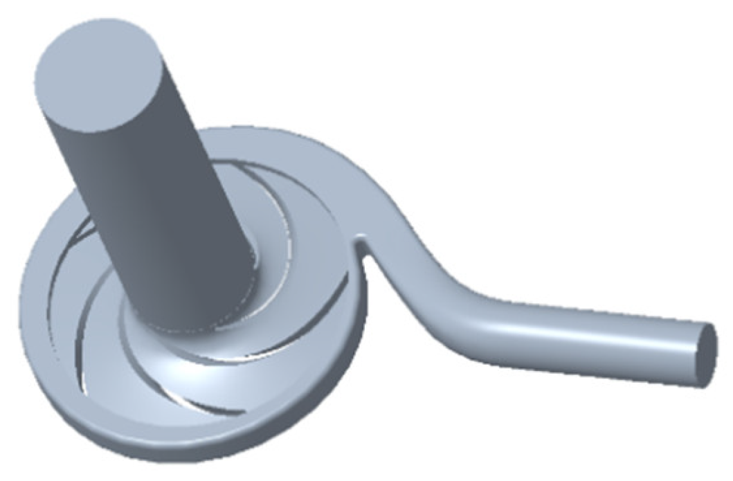
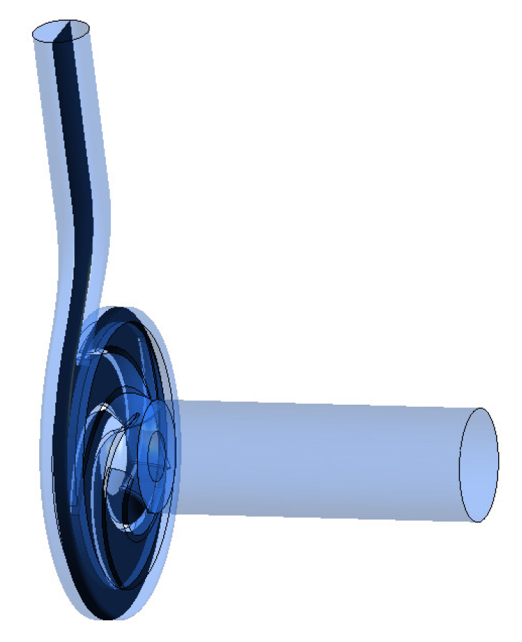
3.1. Pump Model

This study takes an OHA single-stage single-suction centrifugal pump as the research object. The rated flow rate of the pump and the rotation speed were 60 m³/h and 2910 r/min, respectively. The specific speed (n_s = nQ^0.5/H^0.75) of the studied pump model was about 15. The inlet diameter of the inlet pipe and impeller was 100 mm. The outer diameter of the impeller and the outlet width of impeller were 235 mm and 9 mm, respectively. Moreover, the blade number was 5, the inlet width of the volute was 17 mm, while the outlet diameter was 50 mm. The fluid domain was constructed by Unigraphics NX commercial software which was divided into three parts for a complete pump: inlet pipe, impeller and volute. This done to simplify the flow domain and reduce the interfaces to avoid problems and errors when combining the CFD–PBM with the multiphase flow model. The entire water domain is shown in Figure 2 and the numerical settings under single phase is shown in

Table 1. Computational setup under single-phase.

Boundary Conditions
Location	Boundary type	Mass and momentum
Inlet of inlet pipe	Velocity–inlet	Velocity
Outlet of volute	Pressure–outlet	Static pressure
Physical surfaces	Wall	No-slip
Rotor–stator interfaces
Transient state		Transient Rotor–stator
Turbulence model
SST k-ω
Solver control for transient simulation
Timestep		1.7182 × 10−4 s (14 cycles)
Total time		0.288 s
RMS residual		10−5

.

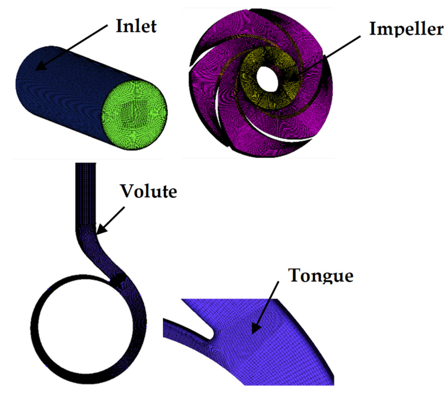
3.2. Mesh Generation

ICEM was used to divide the grid, while the hexahedral structural grid was used for each flow domain. The quality of the grids was all greater than 0.6 (>0.2) with an angle greater than 20° (>14°), which was far above the basic requirement [32]. Under the design flow rates of the single-phase water condition of grid independence analysis, specific results were shown in

Table 2. Mesh independency.

Grid Number/106	Head (m)	Efficiency	Outlet Velocity (m/s)
2.66	71.7645	0.715834	8.662
3.35	72.3672	0.719333	8.608
4.00	72.2497	0.718956	8.632

. The table shows that when the grid number was increased from 3.35 to 4.00 million, the hydraulic head, efficiency and outlet velocity deviation was all less than 1%. To maximize computational resources and simulations, a grid with 3,345,530 cells was finally chosen. The grid number of the impeller, volute and inlet pipe was 1,775,875, 1,068,184 and 501,471, respectively. Figure 3 shows the detailed mesh view of each flow domains meshed with structured grids. The definition of head and efficiency are show in Equations (11) and (12).

$$H=\frac{P_{static,out}-P_{static,in}}{\rho g}.$$

(11)

$$\eta =\frac{\rho gQH}{Mw}.$$

(12)

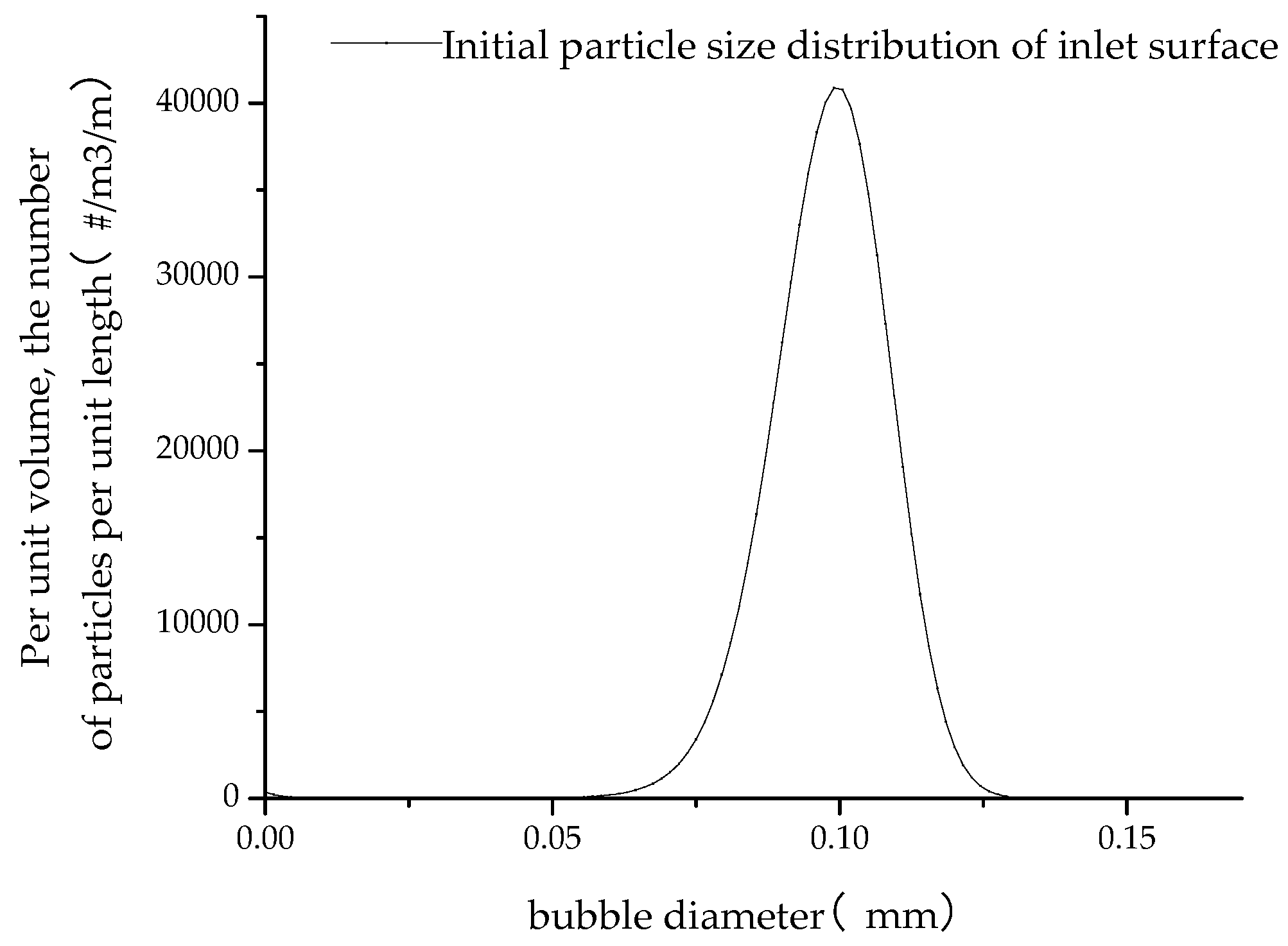
3.3. Gas–Liquid Two-Phase Flow Calculation Settings

The gas–liquid two phase flow correction CFD–PBM was set up using the transient calculation with convergence precision of 10⁻⁵. Due to the direct use of the PBM, an overflow or divergence occurs during the calculation. Thus, the following procedures are proposed: First, use the conventional Eulerian–Eulerian heterogeneous flow model; choose the SST k-ω turbulence model; in the boundary condition, choose velocity–inlet and pressure–outlet and proceed with the calculation until the inlet pressure and outlet velocity have a stable fluctuation. Finally, switch to the PBM. Furthermore, the relative position between the impeller and volute is updated at each timestep which has the values of 1.7182 × 10⁻⁴ s, equivalent to the time interval for the impeller to rotate by 3°, respectively. The cycles of conventional model calculation stage and the PBM calculation stage were 14 and 7 for each stage with a total time of 0.288 s and a total step size of 1680 steps. The data for the last cycle was selected on the average calculation for all the hydraulic performance results.

4. Calculation Results and Analysis

4.1. Validation of the CFD–PBM

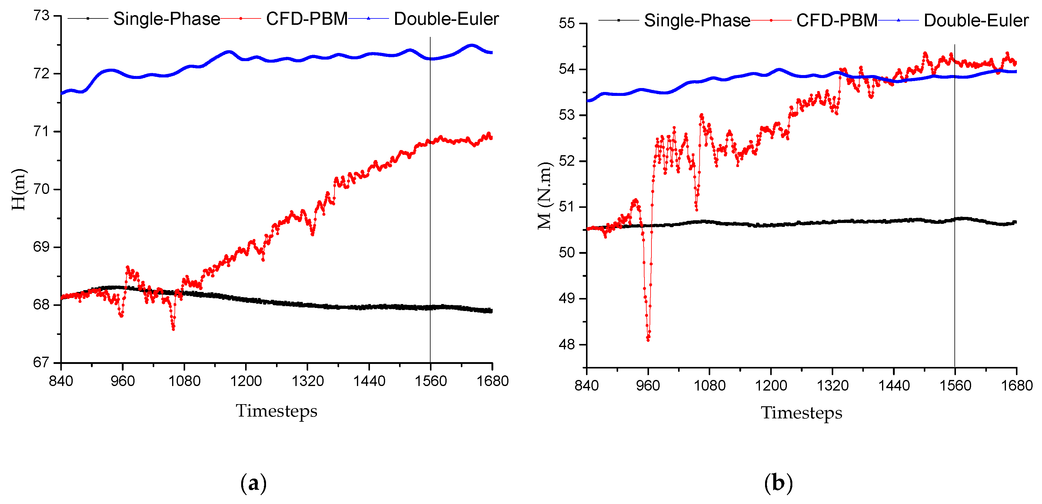
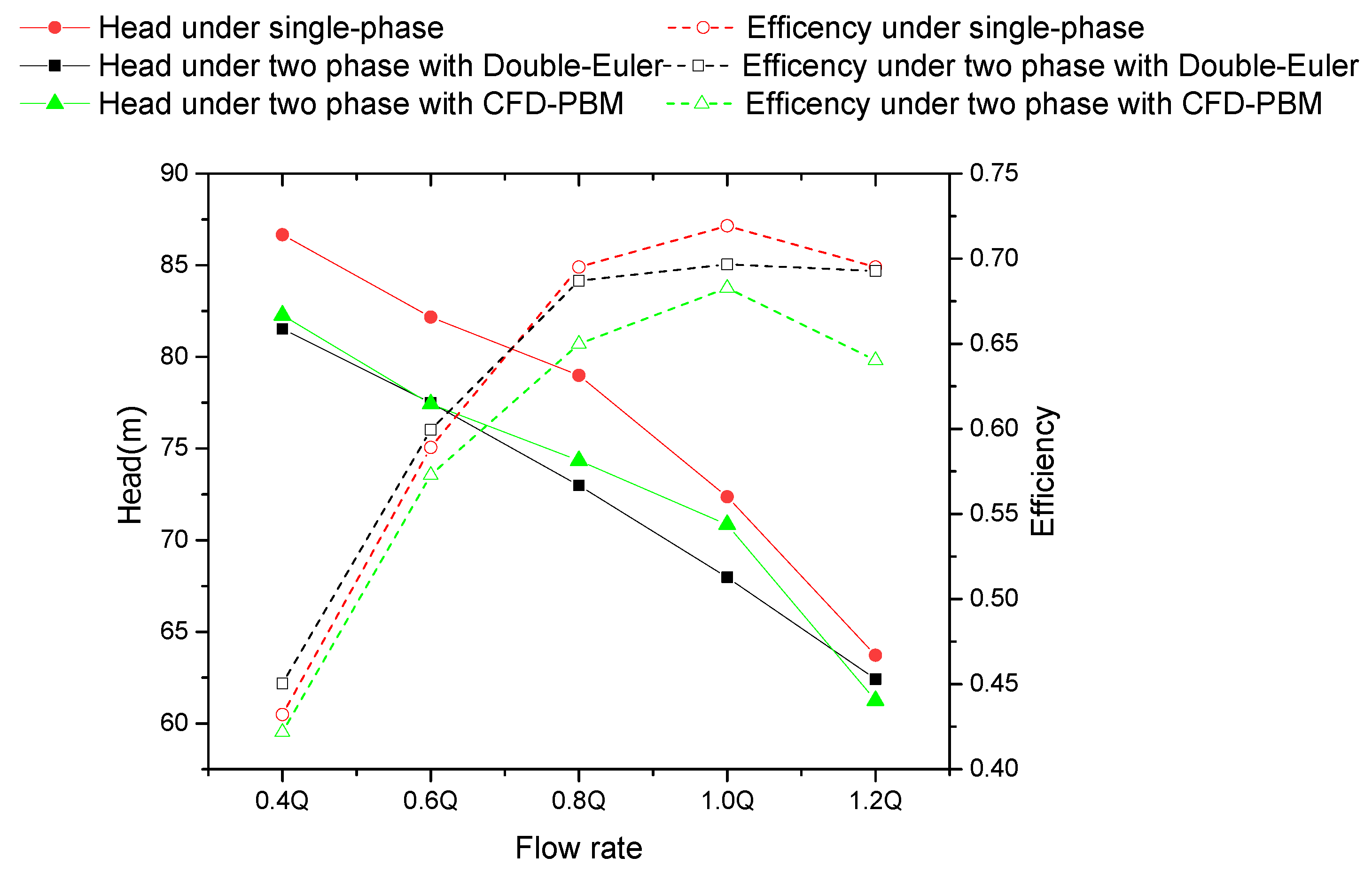
4.1.1. Comparison of Hydraulic Performance Using Different Multiphase Models

Figure 4 shows the head and torque fluctuation under 1.0 Q after adding the CFD–PBM, which starts from 840 time-steps, equivalent to 0.144 s. Comparing the head and torque curves using different multiphase models, the trend was the same at the first 60 timesteps, this was because the diameter of bubbles did not obviously change. The curve then severely fluctuated and the deviation between these two models became large. Finally, the trend turned to basically even, without significant change.

Figure 5 shows the hydraulic performance comparison of a single-phase and gas–liquid two-phase flows using the CFD–PBM and Double Euler (inlet gas volume fraction was 3%). Results of each working condition were obtained after averaging the stable data in the last period of transient calculation. It can be seen from Figure 5 that the hydraulic head of the centrifugal pump significantly decreased in gas–liquid two-phase flow conditions using both models, especially in the case of a small flow rate. The drop range was up to 5 m while the drop range was about 2 m with the CFD–PBM and 4 m with Double Euler, in the case of 1.0 Q. From an overall scene, the head curve was similar, which suggested the CFD–PBM did not significantly influence the head performance. However, there was a large deviation in the efficiency of two multiphase model especially when the flow rate was large. It was found the value of pump efficiency using Double Euler was almost the same as single-phase although the head significantly decreased. From Si [36], the hydraulic performance would decrease significantly not only head, but also efficiency when IGVF increased to 3%. In addition, under small flow rate, the efficiency under single phase and gas–liquid two-phase flow was almost similar.

Further simulations were carried out for inlet gas volume fraction (IGVF) of 10% and 20%. From Figure 6a, when the inlet gas volume fraction increased to 10%, the head and efficiency reduced to 52.17 m and 56.06%, respectively. Similarly, when the inlet gas content was further increased to 20%, the head and efficiency decreased considerably to 9.46 m and 18.19%, respectively. The trend of hydraulic performance dropped by the CFD–PBM with the change of bubble diameter was similar to the study based on the modified bubble sizes by Zhu [37] as shown in Figure 6b.

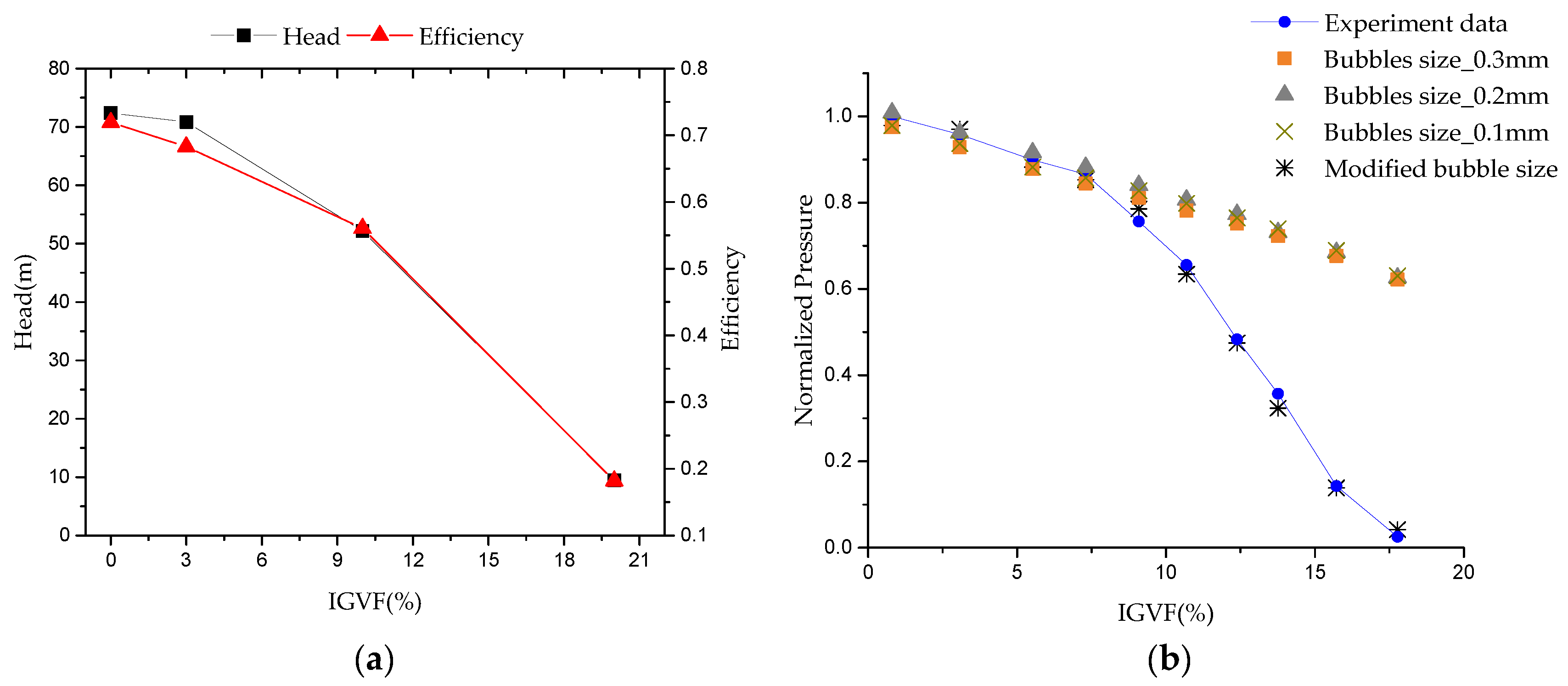
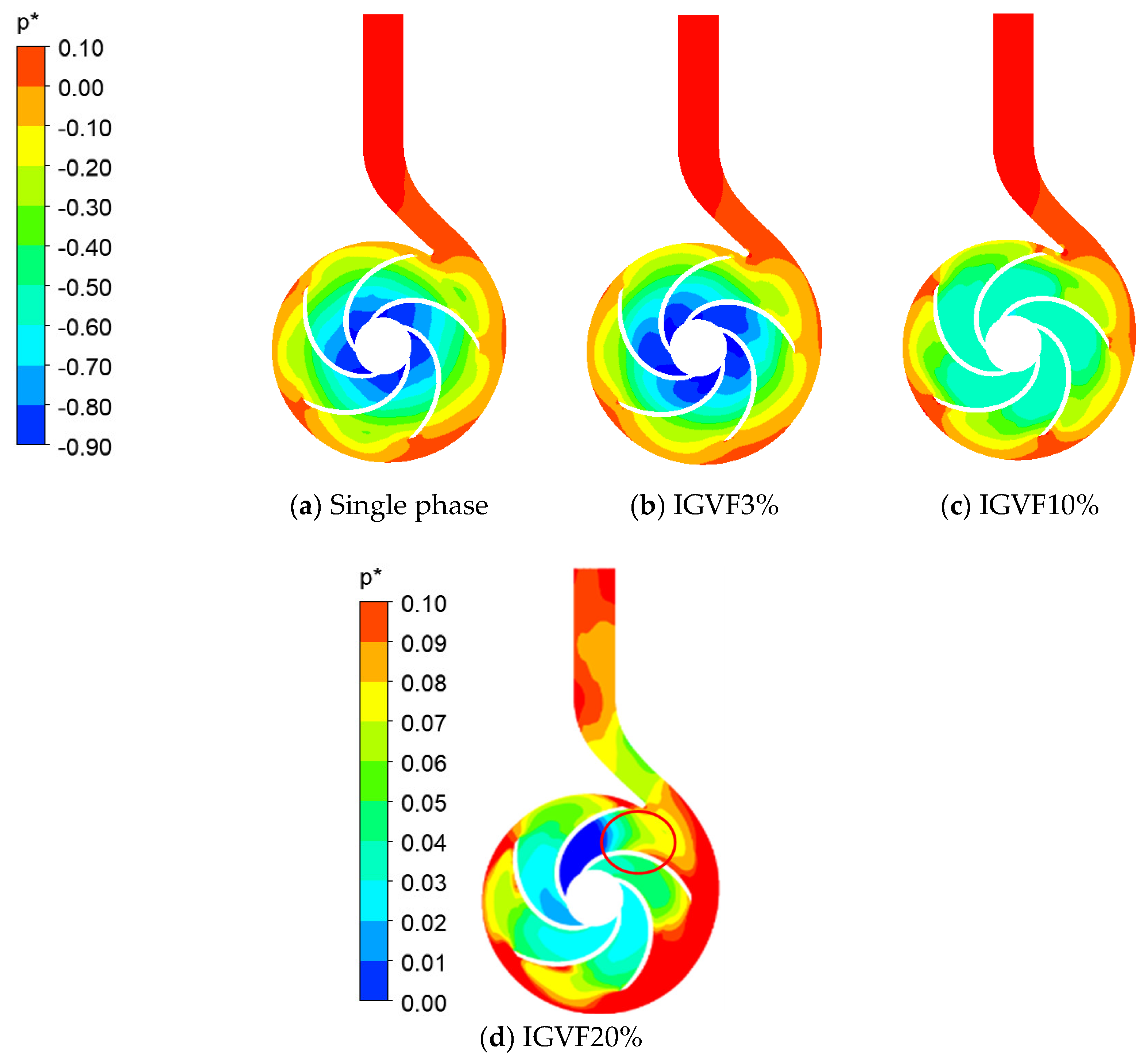
4.1.2. Comparison of Pressure under Different Inlet Gas Volume Fractions (IGVFs)

Figure 7 represents the middle section of the whole pump, the plane was set on the xy plane at z = 0. Figure 8 compares the pressure contour in the middle section of the design flow rate under a single-phase and gas–liquid two-phase under different IGVF. Due to the boundary settings of the velocity–inlet and pressure–outlet, it is clear that static pressure of outlet under different IGVF are the same. Moreover, it can be seen from the figure that the pressure gradient increases from the inner radius to the outer radius of the impeller because the kinetic energy generated from the impeller rotation is converted into potential energy. The largest potential energy occurred in the volute. Under single phase and at IGVF of 3%, the approximation of the distribution of pressure contour showed that low pressure area was mainly concentrated at the inner radius of the impeller. When the IGVF increased to 10%, the pressure at the inner radius increased as well which led to the significant decrease of the hydraulic head. Furthermore, the pressure gradient on the section began to appear uneven. When the IGVF was higher than 20%, the phenomenon of uneven pressure distribution was obvious, particularly in the impeller passage close to the volute where the pressure was much lower. There was even obvious pressure reduction at the volute tongue where the pressure gradient increased. Kosmowski [38] found out that when the IGVF increased over 15%, a phase separation occurred at the impeller outlet causing a rapid change of pressure in impeller passage. And when the IGVF is increased to 20%, the single-stage centrifugal pump cuts out. The highly uneven pressure distribution illustrates that the IGVF was close to the critical value of this pump.

$$p*=\frac{p}{0.5\rho U_2{}^2}.$$

(13)

$$U_2=\frac{\pi nd}{60}.$$

(14)

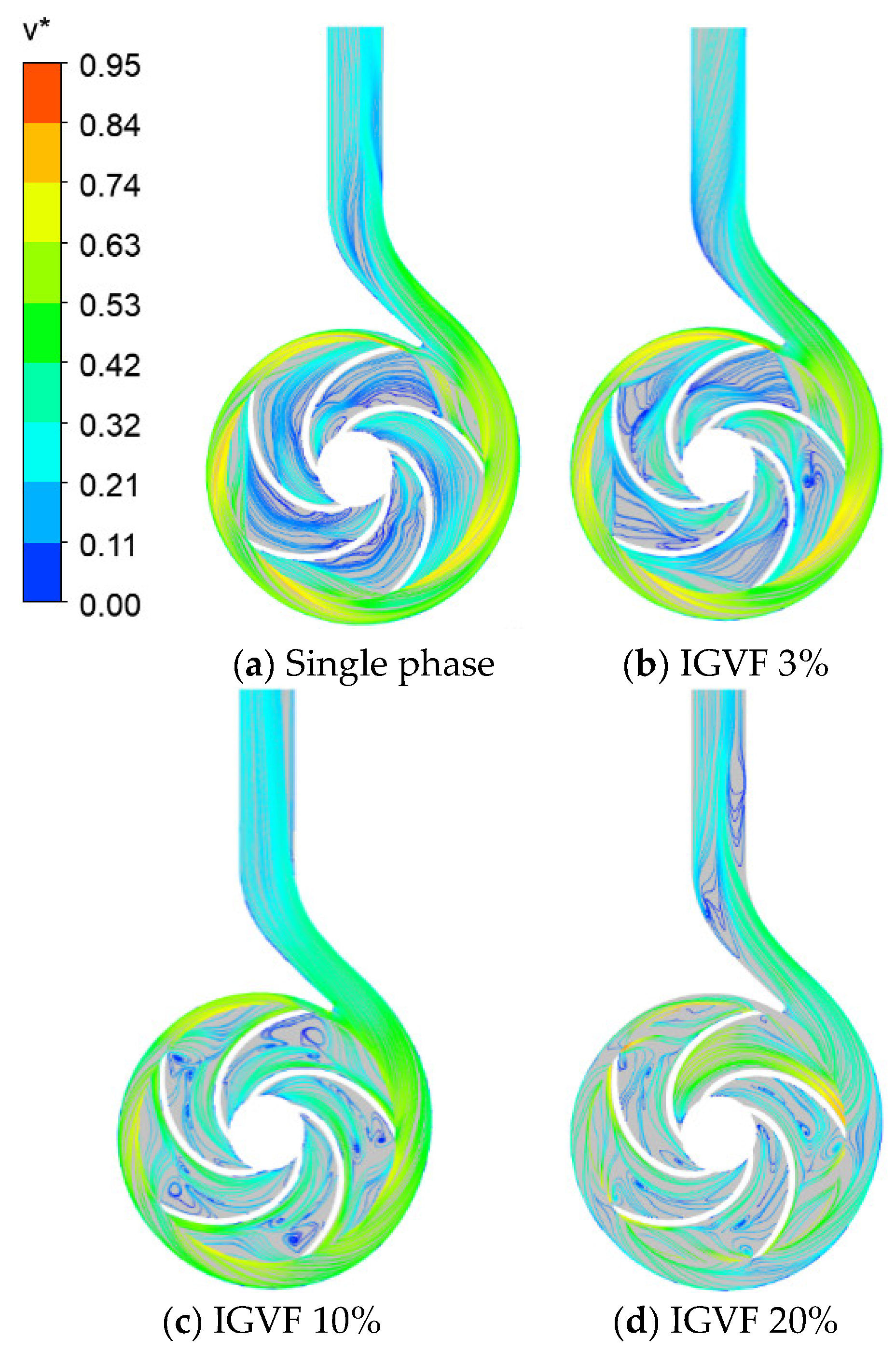
4.1.3. Comparison of Velocity under Different IGVFs

Figure 9 depicts the velocity streamlines of the liquid phase at the middle section under the conditions of single phase under different IGVFs. From the figure, relative to the gas–liquid two-phase flow, the streamline of the liquid phase in the impeller was evenly distributed under single-phase flow. In addition, the inner radius to the outer radius of the impeller was observed to have only small vortices appear near the impeller hub which is closer to the volute. When the IGVF was 3%, the formation of streamlines at the inner radius of the impeller was approximate to a single phase, but the velocity streamlines in the middle part of the impeller concentrated on the working face of blades. The streamlines on the back face of the blades were relatively thinner and the sizes of vortex sprung up in the middle of the impeller passage especially the flow passage in front of and behind the volute tongue which appears a very powerful vortex. When the IGVF was increased to 10%, the vortexes offset to the back face of the blades strengthening the intensity which almost covered the entire back faces of the blade profiles where a large streamline gap area occurred. When the gas content increased to 20%, the flow in the whole area was very disordered. The entire impeller flow passage was full of different sizes of irregular vortices. Two large vortices were observed, which nearly blocked the discharge pipe of the volute. These reasons justify the large drop in the hydraulic performance of the centrifugal pump with a higher IGVF.

$$v*=\frac{v}{U_2}.$$

(15)

4.2. Transient Inner Flow Characteristics under Low IGVF

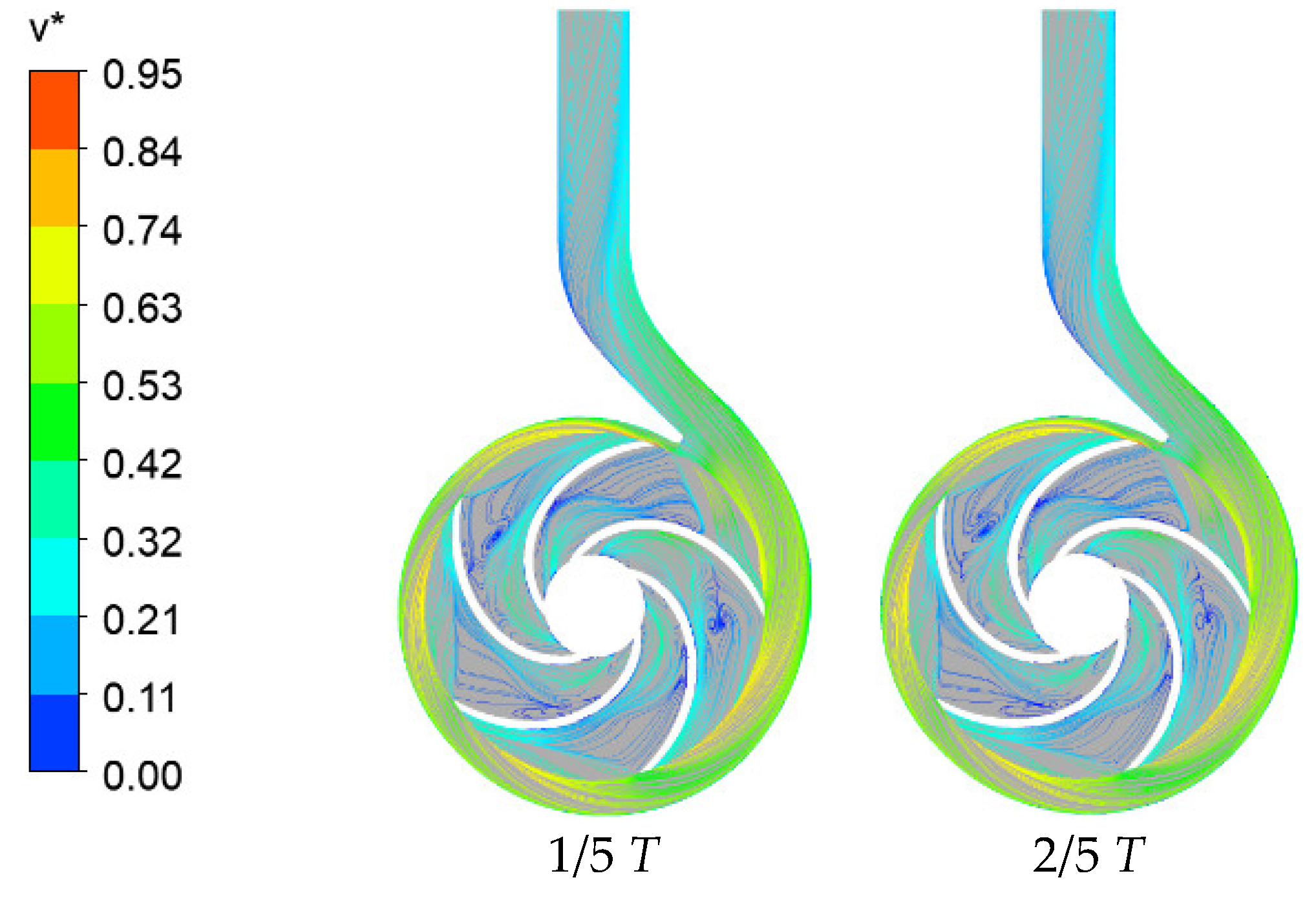
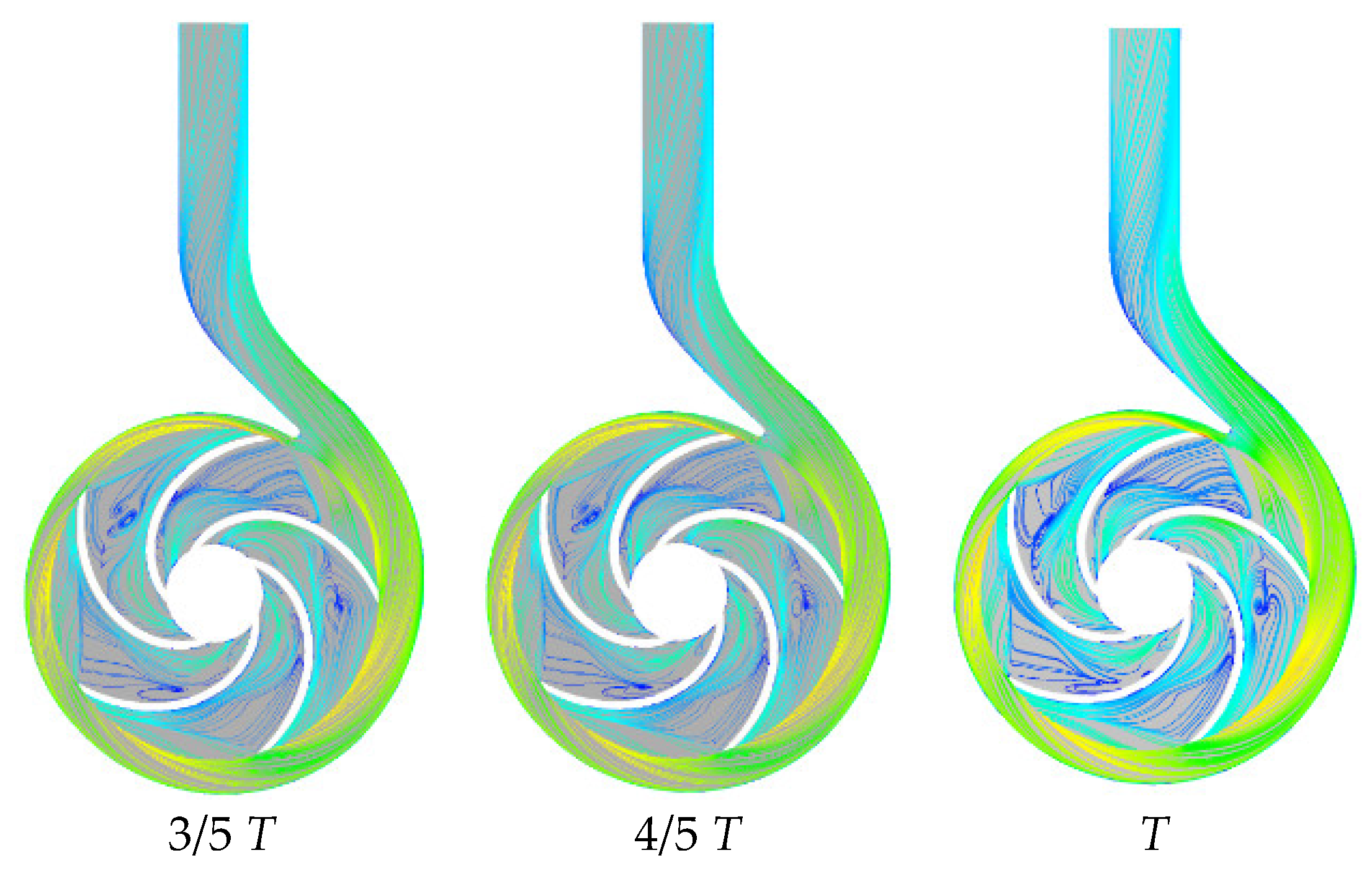
4.2.1. Transient Velocity Distribution at Different Timesteps

The streamlines of liquid phase on the middle section ay different timesteps in one complete cycle under the design flow rate at 3% IGVF is shown in Figure 10. From the inner radius of the impeller to the outer radius of the impeller, the initial trajectory of the liquid phase streamlines slightly offset to the back face while to the impeller middle, liquid phase streamlines were gradually closer to the working face and outer edge. In addition, vortex regions of different sizes appeared at the middle of the impeller.

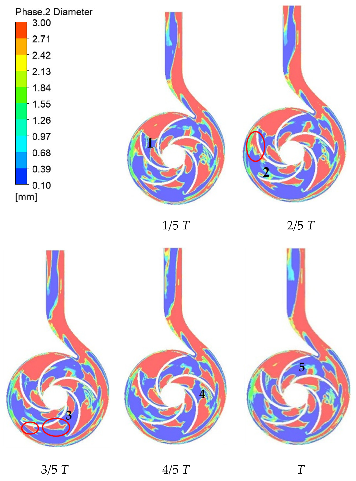
4.2.2. Transient Mean Bubble Diameter Distribution at Different Timesteps

Figure 11 shows the transient mean bubble diameter distribution on the middle section of one complete cycle under the design flow rate when IGVF was 3%. It is apparent that, in the impeller passage, most large-diameter of bubble concentrated in the region at the inner radius of the impeller and the outer radius of impeller while the other small part gathered in the middle of the impeller. Comparison with liquid phase streamline in Figure 8, it was found that where the velocity streamlines had a higher speed or vortex in Figure 8 always existed large-diameter bubbles. It can be known from the laws of hydromechanics that with the increase of the velocity, the pressure of the mixture fluid decreases. Therefore, when the bubbles are subjected to less pressure, the bubble expands, hence, the diameter of the bubble grows.

Moreover, the formation of flow in the impeller passage flow of bubbles was likely to be between bubble agglomerated flow and gas pocket flow [8], because there were large-diameter bubbles concentrated on the inner and outer radius of the impeller. The dispersed phase interaction promotes the aggregation and coalescence of some bubbles leading to the formation of larger diameter bubbles. At this time, the larger bubbles formed by coalescence was irregular. It is apparent from Figure 9 that the large-diameter bubbles almost fixed near the inner radius of the impeller. This is because the pressure at the inner radius is the lowest in the impeller passage which makes the bubbles easily expand causing the formation of an area with large-diameter bubbles. In the downstream turbulent wake area, the characteristics of this area were mainly the accumulation of small bubbles separated from the mainstream which formed into a strong recirculation area. Due to the inertial force effect, the area where large-diameter bubbles occurred became closer to the impeller working face. In contrast to the outer radius of the impeller, it was found that the areas where bubbles with large-diameter concentrated on were in the flow passage which occurred in front of and behind the volute tongue. These were much larger than two flow passages remote from the volute tongue. This was because when the fluid flows near the tongue, there was a disorder in the movement producing large number of bubbles to coalescence, eventually leading to the large diameter of bubbles. However, given that more bubbles concentrated on the passage close to the volute tongue and then flows out directly with the liquid phase which could not enable a large area of large-diameter bubbles to be formed.

Taking the diameter of bubbles distribution change at the middle section in one complete cycle, for instance, in 1/5 T, position 1 was an area concentrated with large-diameter bubbles. From the velocity streamlines in Figure 10, it could be seen that in the middle of the impeller, a strong vortex was formed. This vortex caused the small bubbles produced by the unstable flow coalescing to be large diameter bubbles. This area connects between the middle radius of impeller with outer radius of the impeller, hence causing a large area with large-diameter bubble. In 2/5 T, position 1 rotate to position 2, the velocity streamlines here were relatively smooth. Breakage of part of the large-diameter bubbles occurred due to flow shear and merely. The large gathering area formed in the last period gradually separated because the pressure on the working face of the impeller was higher than the pressure on the back face. Therefore, the large-diameter bubbles concentrated on the back face of the impeller were preferentially broken on the working face. A relatively narrow area concentrated with large-diameter bubbles was formed on the working face of the impeller. In addition, a low-intensity vortex was also found at the back face of impeller by comparing velocity streamlines at the same place. The bubble aggregation area was more scattered, and the average diameter was much smaller than the intensity vortex areas. When the blade was rotated to 3/5 T of a period, the previous in 2/5 T the separate two long and narrow bubble gathering areas were broken into two parts one at the outer radius and the other one at the middle radius of the impeller due to bubble breakage, and the bubble aggregation area at the middle radius of the impeller produce certain irregular deformation. And then the impeller rotated to 1/5 T again, where a large bubble aggregation area similar with that of position 1 appeared. Finally, as the fluid flows out of the impeller and flows through the tongue to the outlet of the volute, large diameter bubbles also flew out along with the transmitted water. The diameter distribution contour of bubbles in position 5 was different from what positions 1 and 4 portray.

Figure 12 shows results from previous literature [8,36,39], there is gas-pocket flow representing that bubbles here coalesce together as large-diameter bubbles always at the inner radius and outer radius similar. This is similar to the numerical results. Due to the limitation of visualization equipment, the rotational speed was kept below 1500 r/min because bubbles produced by high rotational speeds cannot be distinctly captured. Thus, the CFD–PBM had certain applicability to predict the diameter distribution of bubbles in the centrifugal pump.

4.3. The Mean Bubble Diameter Distribution in the Whole Computing Domain

Figure 13 indicates the mean bubble diameter distribution in the whole computing domain and major parts when the gas–liquid two-phase flow occurred in the centrifugal pump. Due to the mix, the fluid flowed steadily and uniformly in the straight inlet pipe. The bubble diameter in most areas of the inlet pipe was equal to the initial set diameter of 0.1 mm. Because the centrifugal pump was cross-axle, there was a sudden contraction in the interface between the inlet pipe and the impeller. The disorder flow produced a certain amount of large diameter bubbles, as shown in Figure 13b of a torus. However, after entering the impeller, the bubble diameter on the shroud and hub became smaller, but the narrow and long large-diameter aggregation areas appeared near the blade surface of each blade—generating a stronger aggregation degree at the inner radius of the impeller. At the same time, compared with the impeller, the aggregation degree of large-diameter bubbles in the volute was obviously greater than that in the impeller. This was because the centrifugal force effect on the impeller rotation and the formation of large-diameter bubbles in the flow was easier to coalesce to the outlet of the impeller. Second, at the interface between the impeller and the volute, there was a large area where large-diameter bubble concentrated on. This could be attributed to the fact that, the fluid in the impeller was affected by the rotation of the impeller causing rotor–stator interaction between the impeller and volute. Moreover, a large gathering area was also formed close to the volute tongue.

Figure 14 shows the value of the average diameter of bubbles on the main surface as shown in Figure 13. The value on the inlet was constant at 0.1 mm, equal to the initial diameter. The average diameter on the blade surface and rotator-stator interface was even double or triple than shroud and hub, which was the same as the overall scene in Figure 13. The fluid near the blade surface got pressurized on the working side and suction on the back side, this surface was the main part for exchange energy. This made the diameter of bubbles easy to coalesce here. In addition, the rotor–stator interface was covered by the areas of the large-diameter bubbles, so the value on the interface was relatively high. Finally, the value on the outlet was the highest of these surfaces, the general trend of average diameter was increased from inlet to outlet.

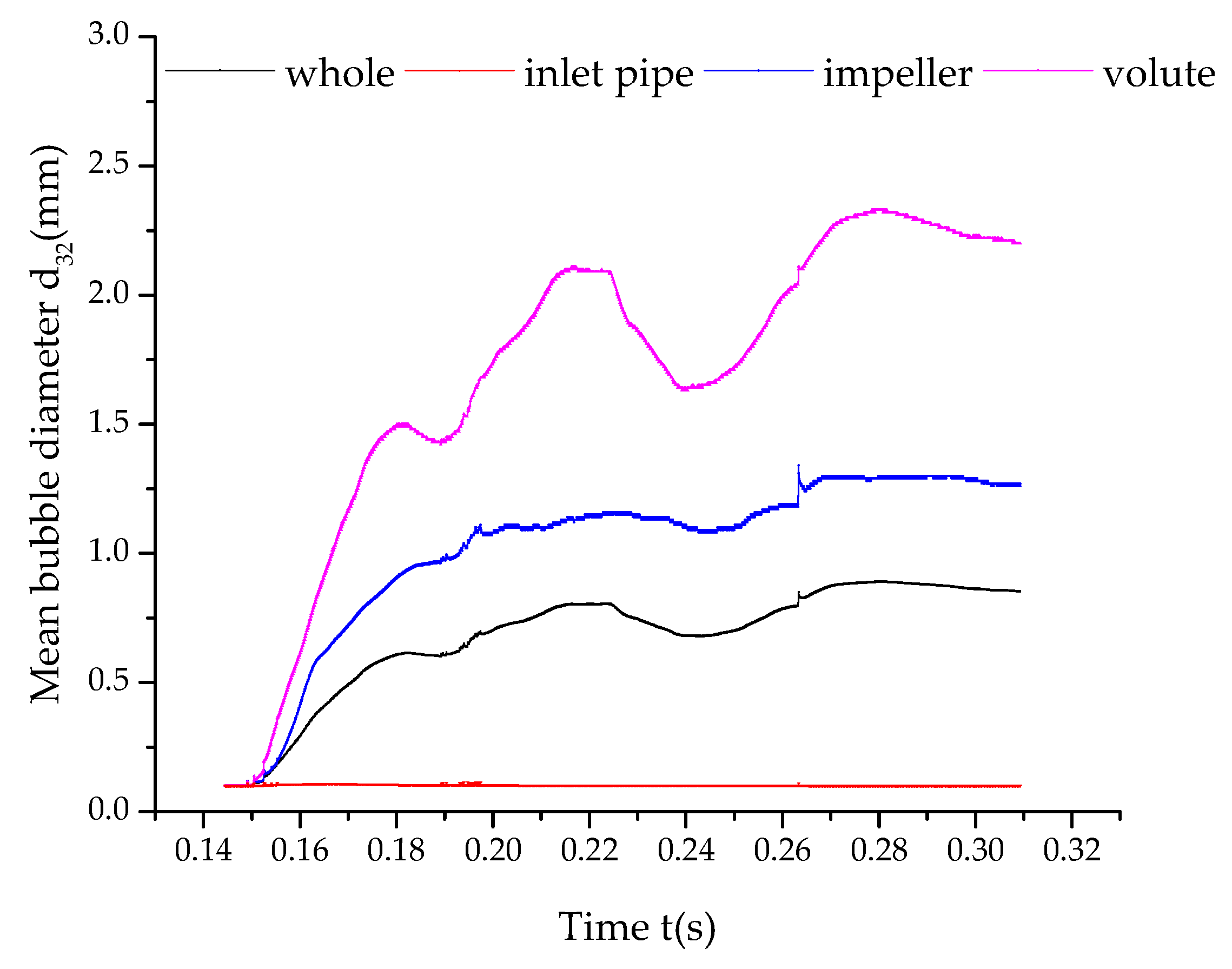
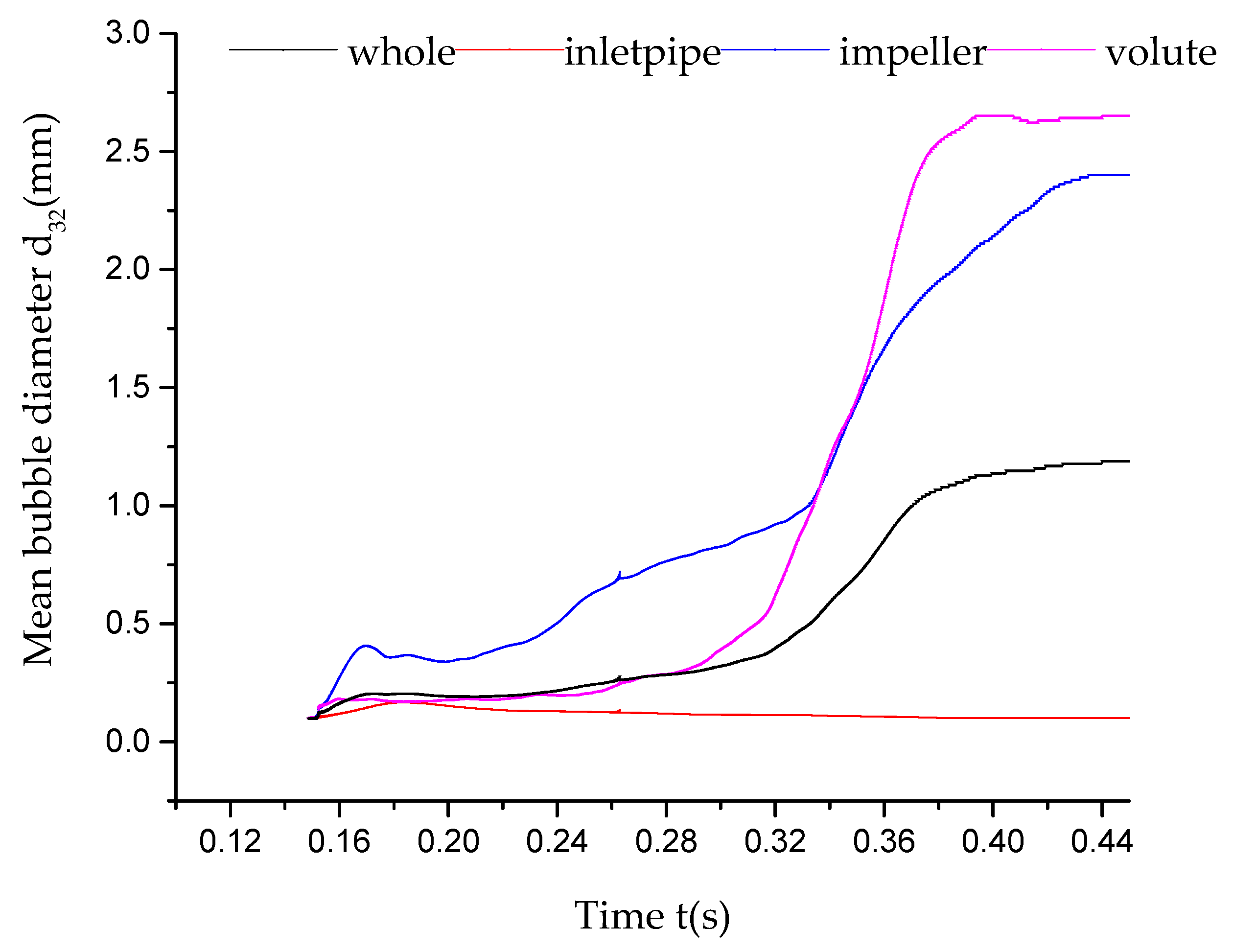
4.4. Variation of the Mean Bubble Diameter with Time

Figure 15 shows the changes of the mean bubble diameter of each domain under design flow. In order to reduce the errors, the PBM was introduced after the flow under gas–liquid two-phase using Eulerian–Eulerian homogeneous flow model after the calculation can process well to avoid overflow or divergent. It can be seen from Figure 11 that except for the inlet pipe, the bubble diameter inside the impeller and volute presents an obvious upward trend and finally tends to be stable. Since the inlet pipe was straight, the bubble diameter did not change entirely and only a fraction of the positions exhibited calculated fluctuations. Between 0.14–0.18 s, the impeller and volute bubble coalescence rate were greater than the bubble breakage rate such that the air bubble diameter rose rapidly. Then in the 0.18–0.22-s period, the growth of bubble diameter in the impeller was slow. The rate of bubble breakage within 0.24–0.26 s was greater than the bubble coalescence rate; thus, the diameter of bubbles reduced and formed a trough. Compared with the impeller, the volute was more unstable rendering the curve of the volute with multiple peaks and troughs. Hence, the PBM could be used more clearly to reflect the gas–liquid two phase flow, especially the bubble coalescence and breakage degree change in real time.

Figure 16 displays the variation of the mean bubble diameter but considered only the coalescence without breakage at various water domain. The overall trend was analogous to Figure 2, where the variation of mean bubble diameter was a process of growth to stability. In the condition of considering coalescence merely, the bubble mean diameter stabilization time was much longer than that of adding both coalescence and breakage models. When the bubble mean diameter of various water domain came to ultimate stability, the final time using only the coalescence model was a little longer than using both coalescence and breakage models. The growth law was also different and the region had an early growth and then fell back at the initial time. During this time, all the bubbles were almost having the small diameter with uneven distribution. There was a big difference in the bubble diameter growth curve of the impeller and volute using just the coalescence model as compared with both models. Generally, the rotating impeller will cause a drastic change in the pressure and shear flow, which makes the bubbles more easily to break than in the static volute. Thus, when merely reserving coalescence equations, the bubbles were unable to break, while the vortexes in the impeller were more than in the volute leading to forming more large-diameter bubbles. This is the reason why the diameter of bubbles increased faster in the impeller than in the volute in as depicted in Figure 15 while it was slower in Figure 16 during the initial period. However, due to the flow space in the impeller is less than in the volute, there was no extra space for the coalescence of bubbles. Thus, the expanding rate in the impeller will slow down to a certain extent at about 0.30 s, and the expand rate of bubbles in the volute surpassed. Meanwhile, as no breakage model was added in the model, with the time flowing, the number of primary bubbles also increased from the initial time when the fluid domain was full of small-diameter bubbles. These bubbles were concentrated or expanded to be large-diameter bubbles due to pressure or velocity change and the influence of vortex. At the same time, large-diameter bubbles also kept coalescing. As it was shown in Figure 12, from 0.3 s to 0.4 s, it is observed that small-diameter bubbles coalesced into large diameter bubbles while large-diameter bubbles coalesced into larger-diameter bubbles. It could be seen that the overall trend grew exponentially with the average diameter of bubbles in the impeller and volute increasing rapidly. Since the initial maximum diameter of bubbles is 3 mm, individual bubble diameter that increases to the maximum no longer coalesce and as such, large-diameter bubble and small-diameter bubble formed an equilibrium state.

5. Conclusions

(1)

The entire study showed the capability of the CFD–PBM in the numerical simulation of gas–liquid two-phase flow in a vane pump using the law of bubble coalescence and breakage.

(2)

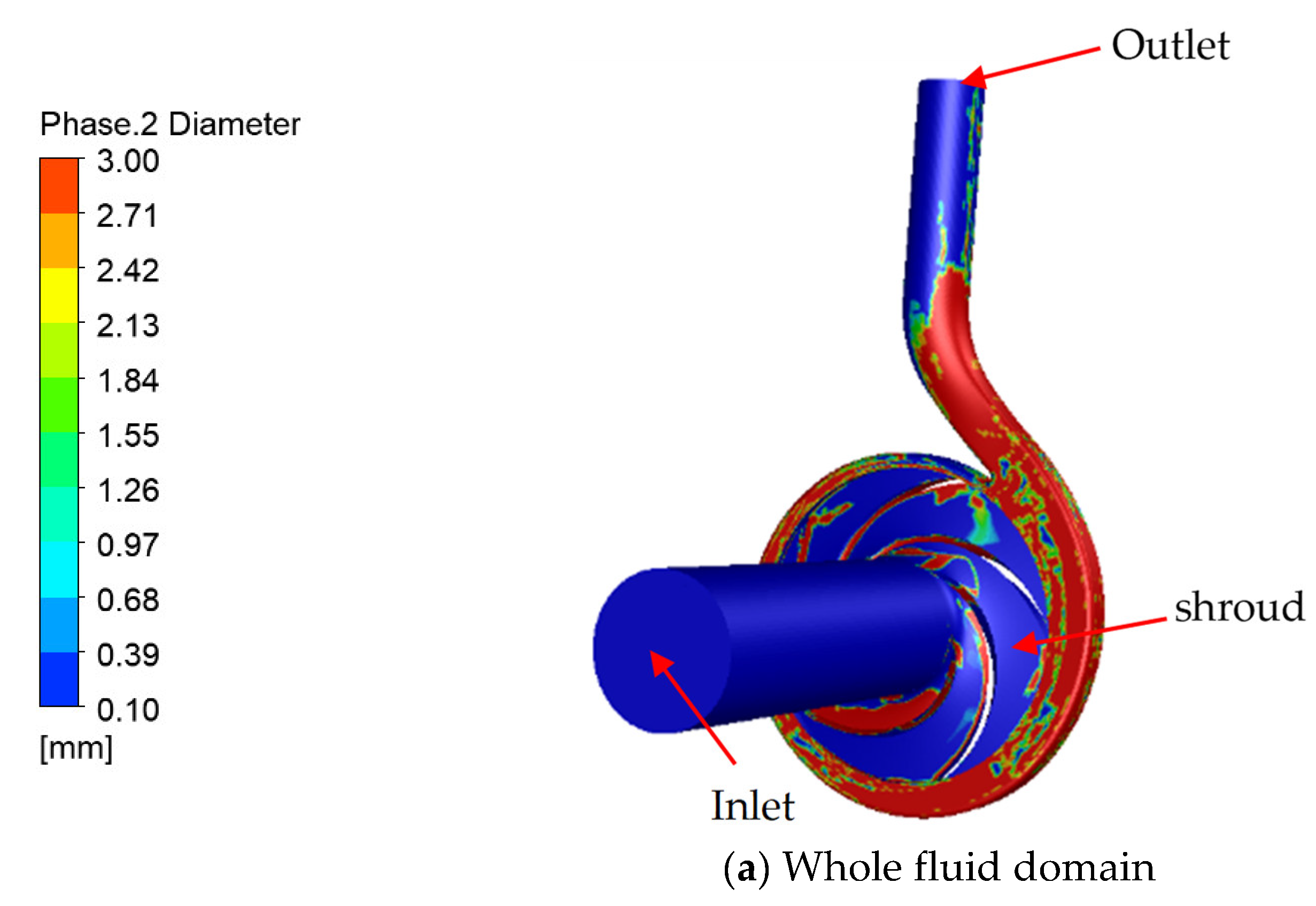
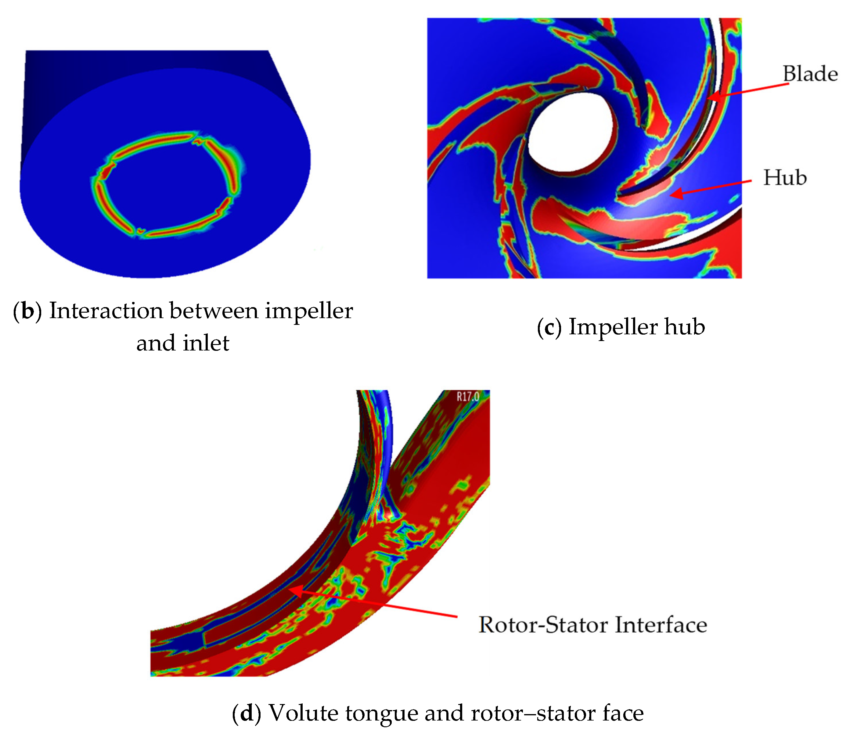
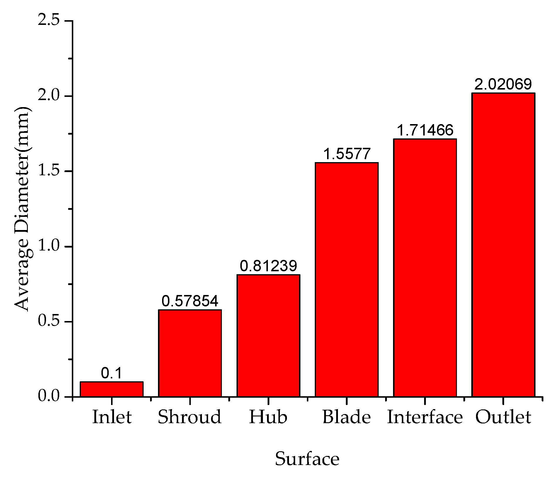
Where the centrifugal pump flow was unstable, bubble concentration was more likely to be produced, forming large-diameter bubbles concentration area to the working face of the impeller. The proportion of large-diameter bubbles in volute was larger than the impeller, and most of them were concentrated in the cavity at the junction of volute and impeller which was related to the rotor–stator interaction between impeller and volute.

(3)

The CFD–PBM could capture the variation of bubble diameter each time. The general rule was that the bubble coalescence rate was much faster than the bubble breakage rate which caused the bubble diameter grow rapidly and enter a steady rising stage. When it finally entered to the equilibrium state, the coalescence rate equaled the breakage rate and the mean diameter of bubbles became stable, which did not fluctuate with time.

From the analysis completed, it can be concluded that the CFD–PBM gave a good prediction of the pump performance and internal bubble diameter distribution under multiphase flow. In a future work, it will be necessary to considerate the influence of bubble size on hydraulic performance and make structural optimization such as split blades or slotted blades focus on where large-diameter bubbles concentrated.

References

1. Johann, F.G. Centrifugal Pumps; Springer: Berlin/Heidelberg, Germany; New York, NY, USA, 2008. [Google Scholar]
2. Pei, J.; Osman, M.; Wang, W.J. Unsteady flow characteristics and cavitation prediction in the double-suction centrifugal pump using a novel approach. Proc. Inst. Mech. Eng. Part A J. Power Energy 2019, 234, 283–299. [Google Scholar] [CrossRef]
3. Tang, S.N.; Yuan, S.Q.; Zhu, Y. Deep learning-based intelligent fault diagnosis methods towards rotating machinery. IEEE Access 2020, 8, 9335–9346. [Google Scholar] [CrossRef]
4. Li, X.J.; Chen, B.; Luo, X.W.; Zhu, Z.C. Effects of flow pattern on hydraulic performance and energy conversion characterisation in a centrifugal pump. Renew. Energy 2020, 151, 475–487. [Google Scholar] [CrossRef]
5. Minemura, K.; Murakami, M. Effects of entrained air on the performance of a centrifugal pump (first report, performance and flow conditions). Trans. Jpn. Soc. Mech. Eng. 1974, 17, 1047–1055. [Google Scholar]
6. Minemura, K.; Murakami, M. Effects of entrained air on the performance of a centrifugal pump (second report, effects of number of blades). Trans. Jpn. Soc. Mech. Eng. 1974, 17, 1286–1295. [Google Scholar]
7. Patel, B.R.; Runstadler, J.P. Investigations into the two-phase flow behavior of centrifugal pumps. Proc Polyphase Flow in Turbomachinery; ASME: New York, NY, USA, 1978; pp. 79–100. [Google Scholar]
8. Verde, W.; Biazussi, J.L.; Sassim, N.A. Experimental study of gas-liquid two-phase flow patterns within centrifugal pumps impellers. Exp. Therm. Fluid Sci. 2017, 85, 37–51. [Google Scholar] [CrossRef]
9. Barrios, L.; Prado, M.G. Modeling two phase flow inside an electrical submersible pump stage. In Proceedings of the ASME 2009 28th International Conference on Ocean, Offshore and Arctic Engineering, Honolulu, HI, USA, 31 May–5 June 2009; pp. 227–231. [Google Scholar]
10. Burrascano, P.; Callegari, S.; Montisci, A.; Ricci, M.; Versaci, M. Ultrasonic Nondestructive Evaluation Systems; Springer International Publishing: Cham, Switzerland, 2015. [Google Scholar] [CrossRef]
11. Caridad, J.; Asuaje, M.; Kenyery, F. Characterization of a centrifugal pump impeller under two-phase flow conditions. J. Pet. Sci. Eng. 2008, 63, 18–22. [Google Scholar] [CrossRef]
12. Marin, M.; Rahmat, E. On solutions of Saint-Venant’s problem for elastic dipolar bodies with voids. Carpathian J. Math. 2017, 33, 219–232. [Google Scholar]
13. Kim, J.H.; Lee, H.C. Hydrodynamic of experiment performance of a multiphase Improvement of pump using design techniques. J. Fluids Eng. 2015, 137, 081301. [Google Scholar] [CrossRef]
14. Wu, Y.L. Three-dimension calculation of oil-bubble flows through a centrifugal Pump impeller. In Proceedings of the Third Internal Conference on Pump and Fan, Beijing, China, 13–16 October 1998; Tsinghua University Press: Beijing, China, 1998; pp. 526–532. [Google Scholar]
15. Zhao, W.G.; He, X.X.; Wang, X.Y. Numerical Simulation of Cavitation Flow in a Centrifugal Pump. Appl. Mech. Mater. 2013, 444, 509–516. [Google Scholar] [CrossRef]
16. Wang, T.; Wang, J. Numerical simulations of gas—Liquid mass transfer in bubble columns with a CFD–PBM coupled model. Chem. Eng. Sci. 2007, 62, 7107–7118. [Google Scholar] [CrossRef]
17. Zhang, B.; Kong, L.T.; Jin, H.B. CFD simulation of gas—Liquid flow in a high-pressure bubble column with a modified population balance model. Chin. J. Chem. Eng. 2018, 26, 1350–1358. [Google Scholar] [CrossRef]
18. Crowley, T.J.; Meadows, E.S.; Kostoulas, E. Control of particle size distribution described by a population balance model of semibatch emulsion polymerization. J. Process Control 2000, 10, 419–432. [Google Scholar] [CrossRef]
19. Chen, X.Z.; Luo, Z.H.; Yan, W.C. Three-dimensional CFD-PBM coupled model of the temperature fields in fluidized-bed polymerization reactors. Aiche J. 2011, 57, 3351–3366. [Google Scholar] [CrossRef]
20. Yan, W.C.; Luo, Z.H.; Guo, A.Y. Coupling of CFD with PBM for a pilot-plant tubular loop polymerization reactor. Chem. Eng. Sci. 2011, 66, 5148–5163. [Google Scholar] [CrossRef]
21. Gu, Z.; Su, J.; Li, Y. Behaviors of the Dispersed Phase in the Multiphase System and Population Balance Model. Chem. React. Eng. Technol. 2007, 23, 162–167. [Google Scholar]
22. Wu, C.F. Study on Distribution and Motion Feature of Salt Out Crystal Particles in Impeller of Centrifugal Pump. Ph.D. Thesis, Jiangsu University, Zhenjiang, China, 2016. (In Chinese with English Abstract). [Google Scholar]
23. Wang, T.; Wang, J.; Jin, Y. Population balance model for gas-liquid flows: Influence of bubble coalescence and breakup models. Ind. Eng. Chem. Res. 2005, 44, 7540–7549. [Google Scholar] [CrossRef]
24. Patruno, L.E.; Dorao, C.A.; Dupuy, P.M. Identification of droplet breakage kernel for population balance modelling. Chem. Eng. Sci. 2009, 64, 638–645. [Google Scholar] [CrossRef]
25. Chen, Y.M.; Patil, A.; Bai, C.R.; Wang, Y.T. Numerical Study on the First Stage Head Degradation in an Electrical Submersible Pump with Population Balance Model. J. Energy Resour. Technol. 2019, 141, 022003. [Google Scholar] [CrossRef]
26. Yan, S.; Sun, S.; Luo, X.; Chen, S.; Li, C.; Feng, J. Numerical Investigation on Bubble Distribution of a Multistage Centrifugal Pump Based on a Population Balance Model. Energies 2020, 13, 908. [Google Scholar] [CrossRef] [Green Version]
27. Menter, F.R. Two-equation eddy-viscosity turbulence models for engineer applications. Aiaa J. 1994, 32, 1598–1605. [Google Scholar] [CrossRef] [Green Version]
28. Zhang, F.; Appiah, D.; Hong, F. Energy loss evaluation in a side channel pump under different wrapping angles using entropy production method. Int. Commun. Heat Mass Transf. 2020, 113, 104526. [Google Scholar] [CrossRef]
29. Wang, Y.F.; Zhang, F.; Yuan, S.Q. Effect of Unrans and Hybrid Rans-Les Turbulence Models on Unsteady Turbulent Flows Inside a Side Channel Pump. ASME J. Fluids Eng. 2020, 142, 061503. [Google Scholar] [CrossRef]
30. Hasse, C.; Sohm, V.; Durst, B. Detached eddy simulation of cyclic large scale fluctuations in a simplified engine setup. Int. J. Heat Fluid Flow 2009, 30, 32–43. [Google Scholar] [CrossRef]
31. Liu, Y.; Hinrichsen, O. Study on CFD–PBM turbulence closures based on k–ε and Reynolds stress models for heterogeneous bubble column flows. Comput. Fluids 2014, 105, 91–100. [Google Scholar] [CrossRef]
32. ANSYS. ANSYS, Release 15.0 ANSYS Documentation; ANSYS, Inc.: Canonsburg, PA, USA, 2013. [Google Scholar]
33. Randolph, A.D. , Larson, M.A. Theory of Particulate Processes; Academic Press Inc.: London, UK, 1988. [Google Scholar]
34. Marchisio, D.L.; Vigil, R.D.; Fox, R.O. Quadrature method of moments for aggregation-breakage processes. J. Colloid Interface Sci. 2003, 258, 322–334. [Google Scholar] [CrossRef]
35. McGraw, R. Description of aerosol dynamics by the quadrature Method of Moments. Aerosol Sci. Technol. 1997, 27, 255–265. [Google Scholar] [CrossRef]
36. Si, Q.R.; Zhang, H.Y.; Gerard, B. Experimental Investigations on the Inner Flow Behavior of Centrifugal Pumps under Inlet Air-Water Two-Phase Conditions. Energies 2019, 12, 4377. [Google Scholar] [CrossRef] [Green Version]
37. Zhu, J.; Zhang, H. CFD Simulation of ESP Performance and Bubble Size Estimation under Gassy Conditions. In Proceedings of the SPE Annual Technical Conference and Exhibition, Amsterdam, The Netherlands, 27–29 October 2014. [Google Scholar]
38. Kosmowski, I. Behavior of centrifugal pump when conveying gas entrained liquids. In Proceedings of the 7th Technical Conference of BPMA, Albany, NY, USA, 15–17 September 1982; pp. 283–291. [Google Scholar]
39. Zhang, Z.D. Experimental study on gas-liquid flow characteristics and pump performance of centrifugal pump impeller under bubble inflow. Master’s Thesis, Xi’an University of Technology, Xi’an, China, 2019. [Google Scholar]
Figure 1. Initial diameter distribution of inlet.
Mathematics 08 00769 g001
Figure 2. Computational flow domain of the investigated pump.
Mathematics 08 00769 g002
Figure 3. Detailed mesh view.
Mathematics 08 00769 g003
Figure 4. Head and torque fluctuation under 1.0 Q. (a) head; (b) torque.
Mathematics 08 00769 g004
Figure 5. Hydraulic performance curves of single-phase and gas–liquid two-phase.
Mathematics 08 00769 g005
Figure 6. Hydraulic performance curves under different inlet gas volume fractions (IGVFs). (a) pump in this study; (b) Zhu [37].
Mathematics 08 00769 g006
Figure 7. Middle section.
Mathematics 08 00769 g007
Figure 8. Variation of the mean diameter with time of the main pump components.
Mathematics 08 00769 g008
Figure 9. Velocity streamline distribution under single phase and different IGVF.
Mathematics 08 00769 g009
Figure 10. Velocity streamline distribution under gas–liquid two-phase in one complete cycle.
Mathematics 08 00769 g010aMathematics 08 00769 g010b
Figure 11. Cloud of bubble diameter distribution in one complete cycle under IGVF = 3%.
Mathematics 08 00769 g011
Figure 12. Visualization of bubbles in previous study. (a) Zhang [39] IGVF = 3.47, (b) Si [36] IGVF = 4%, and (c) Verde [8] IGVF = 2.78%.
Mathematics 08 00769 g012
Figure 13. Cloud of mean bubble diameter distribution in the pump flow passage.
Mathematics 08 00769 g013aMathematics 08 00769 g013b
Figure 14. Average of mean bubble diameter in the main surface.
Mathematics 08 00769 g014
Figure 15. Variation of the mean bubble diameter with time of the main pump components.
Mathematics 08 00769 g015
Figure 16. Variation of the mean diameter with time of the main pump components in the coalescence model.
Mathematics 08 00769 g016