Towards Personalized Diagnosis of Glioblastoma in Fluid-Attenuated Inversion Recovery (FLAIR) by Topological Interpretable Machine Learning


Abstract
1. Introduction
1.1. Topological Data Analysis for Radiomics and Tumor Growth Analysis
1.2. Paper Outline
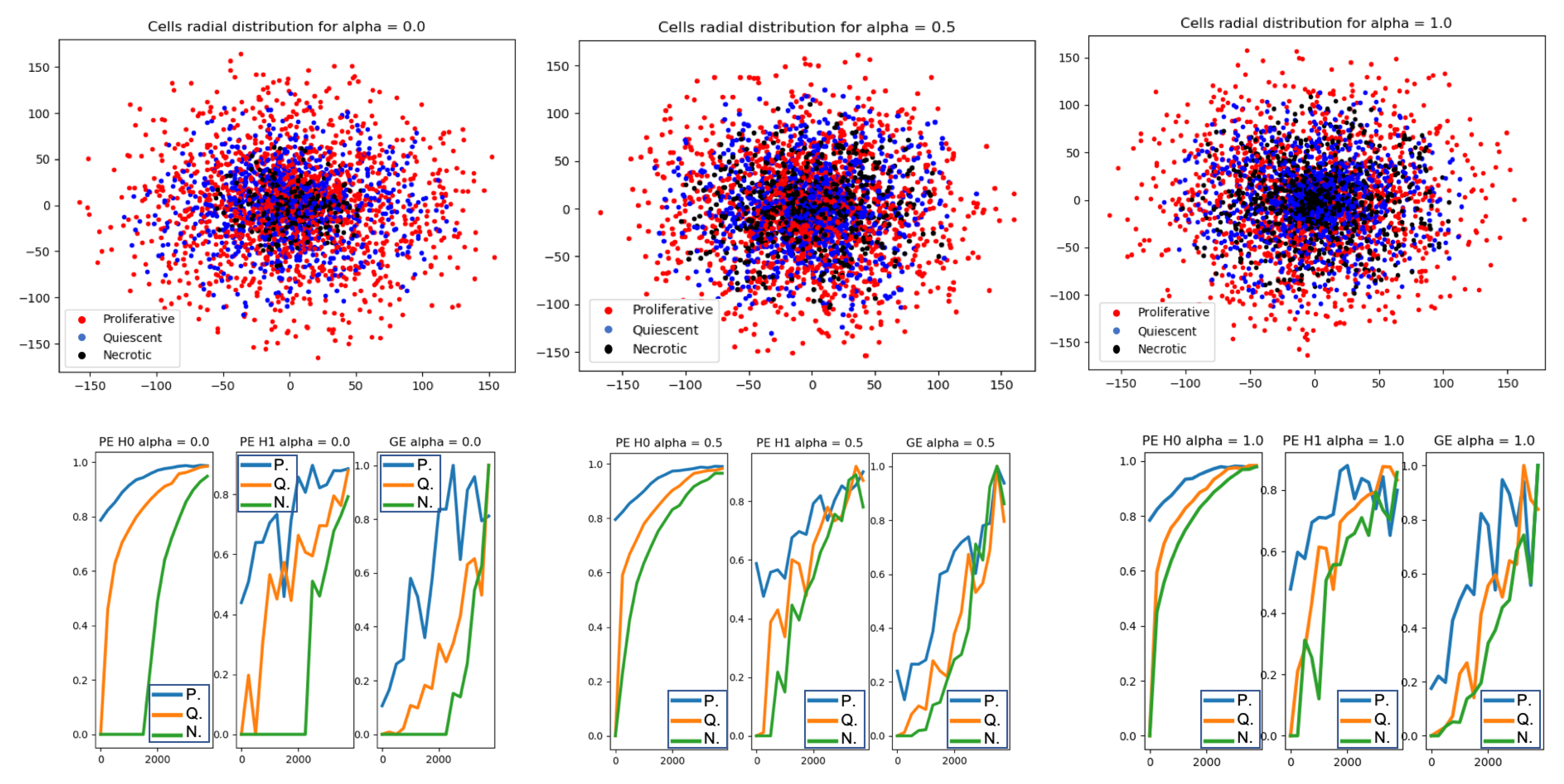
- Analysis 1—Topological Data Analysis of a simplified 2D tumor Growth Mathematical Model: identification how tumor growth over time is affected by the initial amount of available chemical nutrient
- Analysis 2—Topological analysis of Glioblastoma temporal progression on FLAIR: evaluation of GBM temporal evolution after treatment
- Analysis 3—Automatic GBM classification on FLAIR—the aims of this experiment is to evaluate the accuracy for classification GBM by characterization of 2D patches extracted from FLAIR by combining textural and topological data analysis with machine learning.
2. Materials
2.1. Analysis 1: Topological Data Analysis of a Simplified 2D Tumour Growth Mathematical Model
2.2. Analysis 2 & 3: Dataset
2.3. FLAIR Preprocessing
- DICOMs were transformed into NII files for enabling preprocessing steps (https://pypi.org/project/dicom2nifti/).
- FLAIRs were optimized by removing fat tissues and by performing skull stripping. The preprocessing steps, namely the removal of fat tissues and skull stripping, were performed by using the deep-learning algorithm described in Reference [52] (https://github.com/JanaLipkova/s3).
3. Background
3.1. Topological Data Analysis: Persistent Homology
3.2. Topological Features for Radiomics
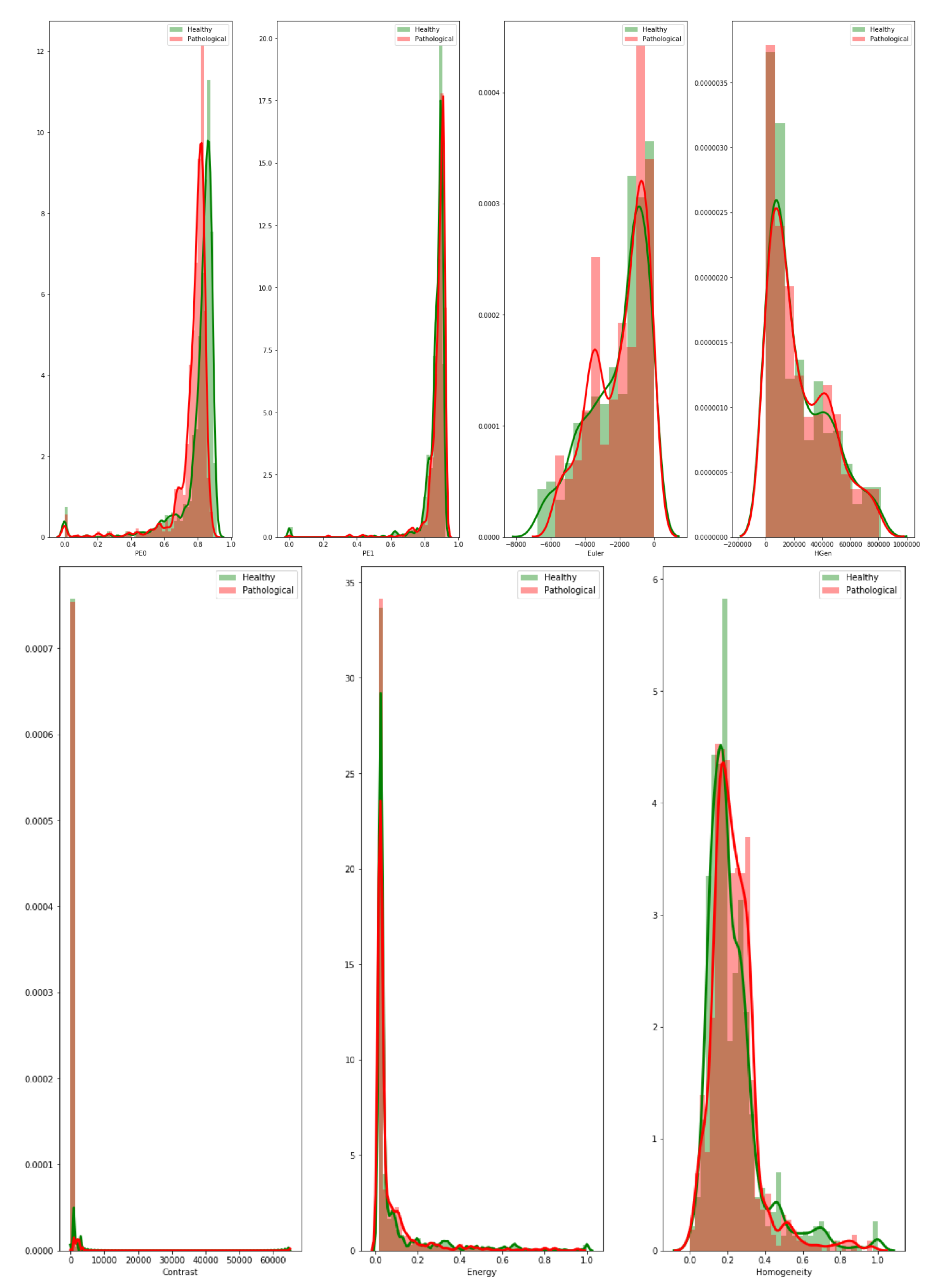
3.3. Textural Features: Grey-Level Co-Occurrence Matrix
- Contrast—it measures the local variability in the grey level.
- Correlation—it measures the joint probability that a given pair of pixels is found.
- Homogeneity—it measures the distance between the GCLM diagonal and element distribution.
- Energy
3.4. Evaluation Metrics
- AUC is the area under the receiver operating characteristics curve (ROC). The ROC is obtained by plotting of the true positive rate () against the false positive rate () at various threshold settings [65].
3.5. Computational Complexity
4. Methods
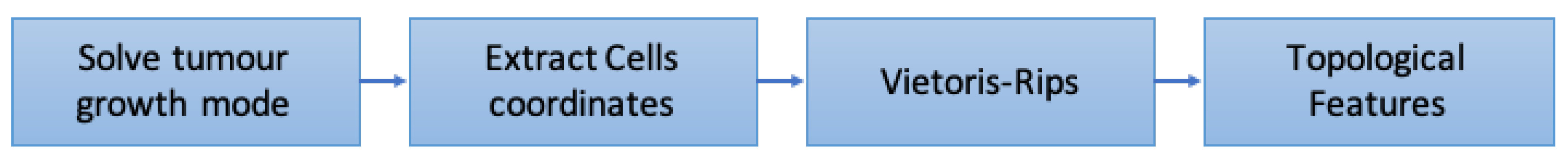
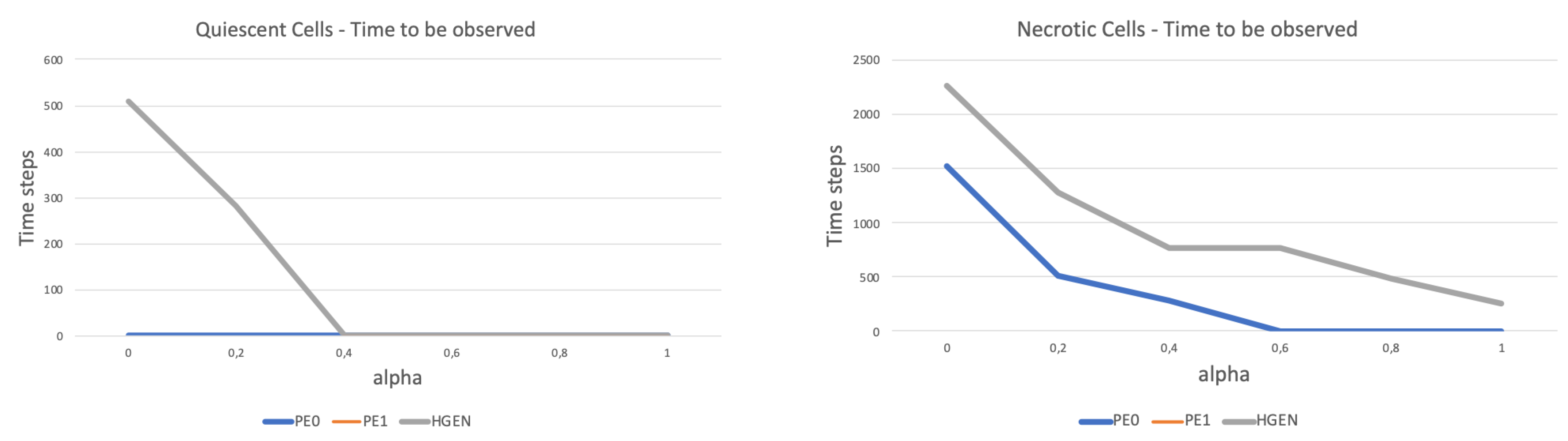
4.1. Analysis 1: Topological Data Analysis of a Simplified 2D Tumor Growth Mathematical Model
- Solve tumor growth model over different .
- Extract cells coordinates.
- Embed the coordinates in a space equipped with the Euclidean metrics and compute Vietoris-Rips simplicial complexes.
- Compute topological features: persistent entropy at H0 and H1, and Generator Entropy.
- Plot the topological features vs .
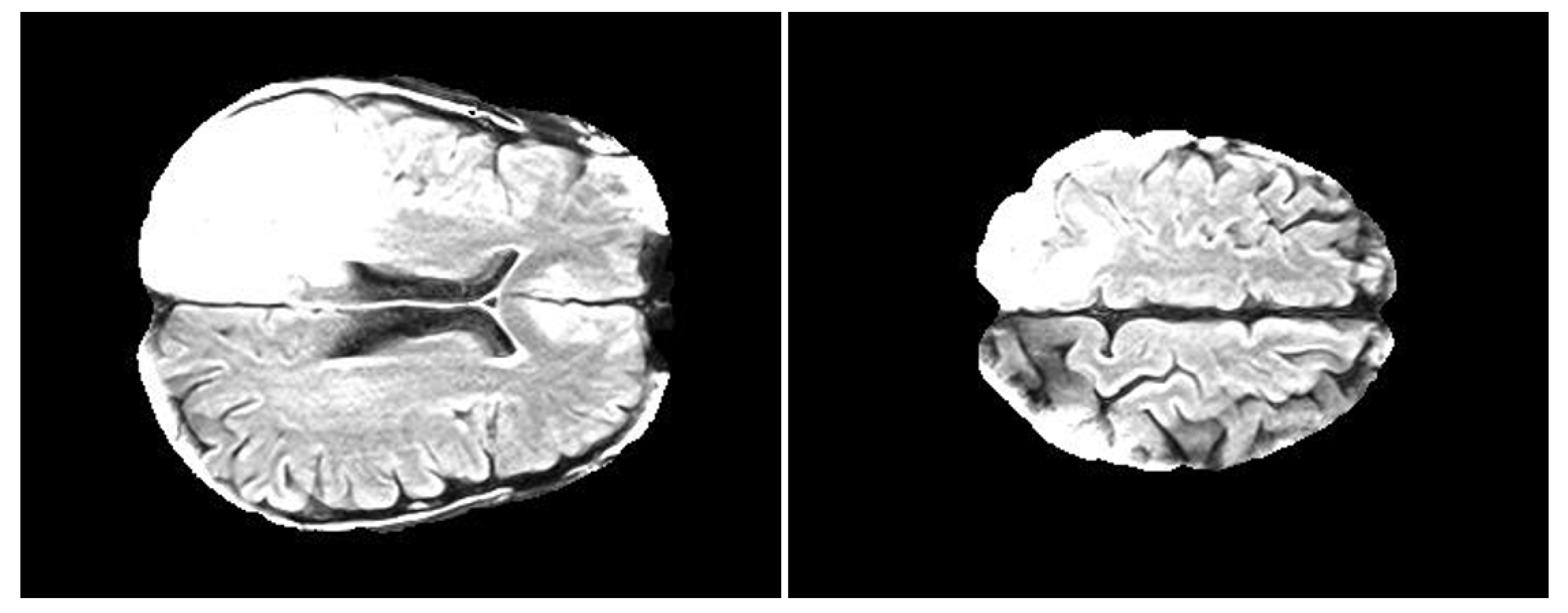
4.2. Analysis 2: Topological Data Analysis of Tumor Progression
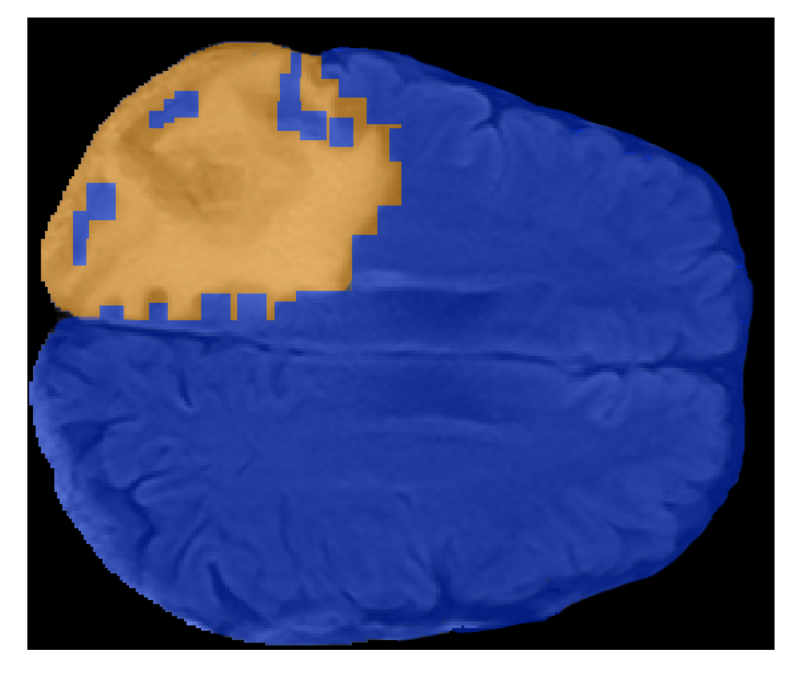
- From both preprocessed “pre” and “post” FLAIRs (i.e., after skull stripping) extract all the slices containing the tumor according to the corresponding ROIs.
- For each slice compute the 2D lower star filtration.
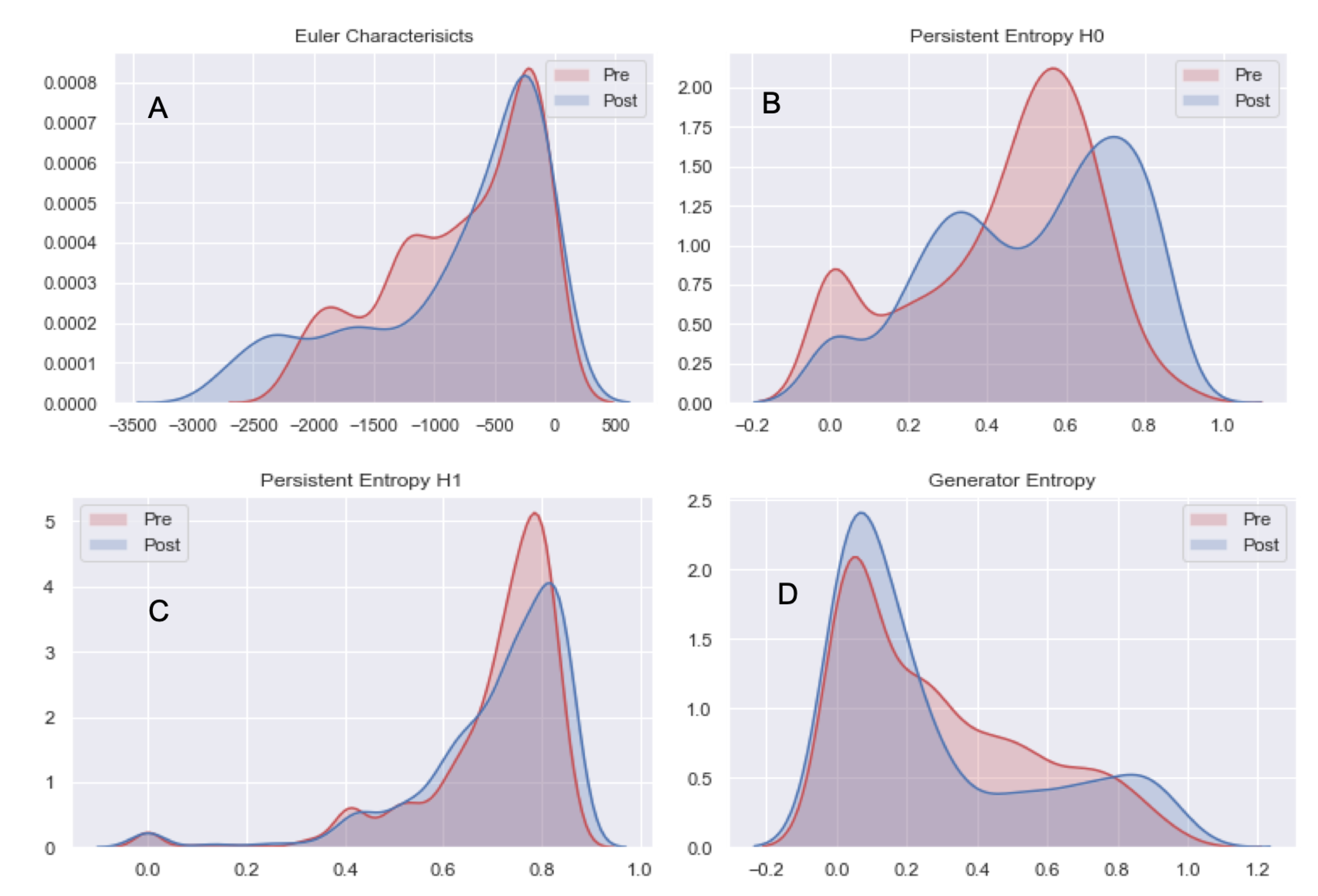
- Compute Topological features: Euler Characteristics, Persistent Entropy at H0 and H1 and Generator Entropy at H1.
- Compare the distributions by using statistical tests, that is, t-test and p-value.
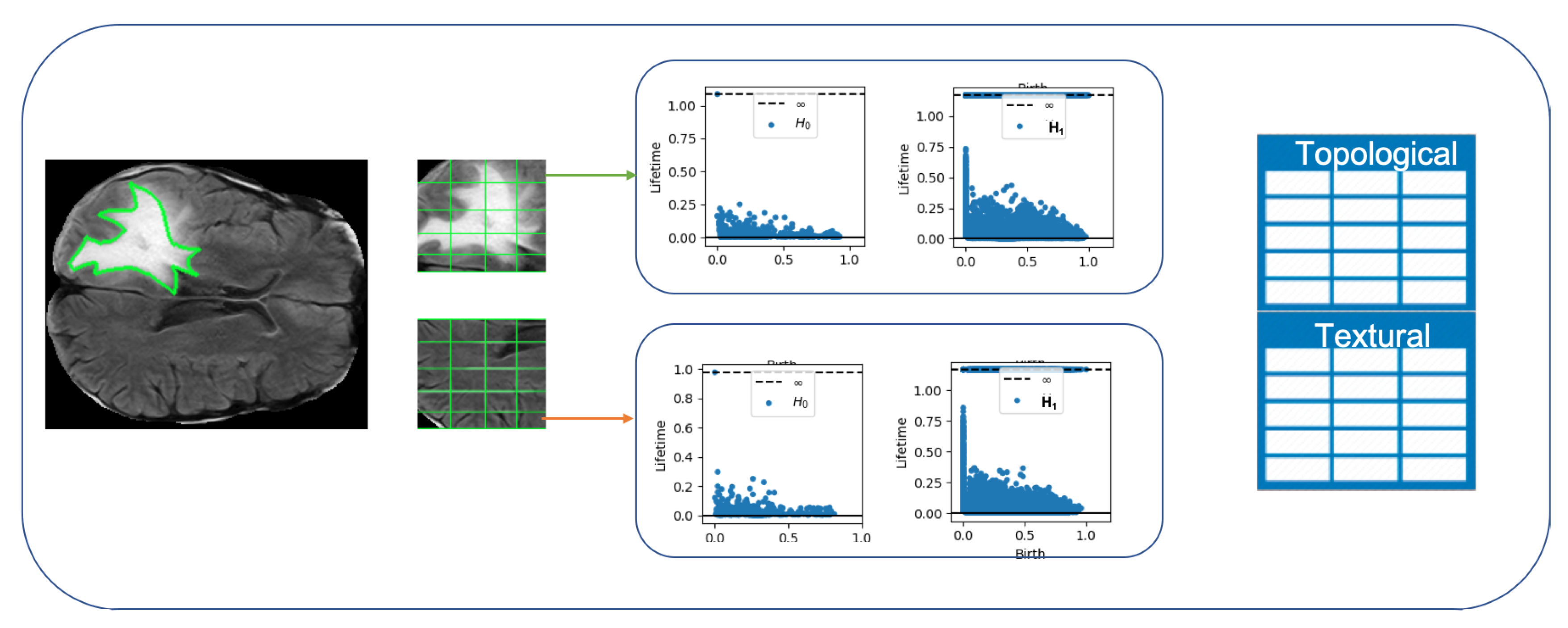
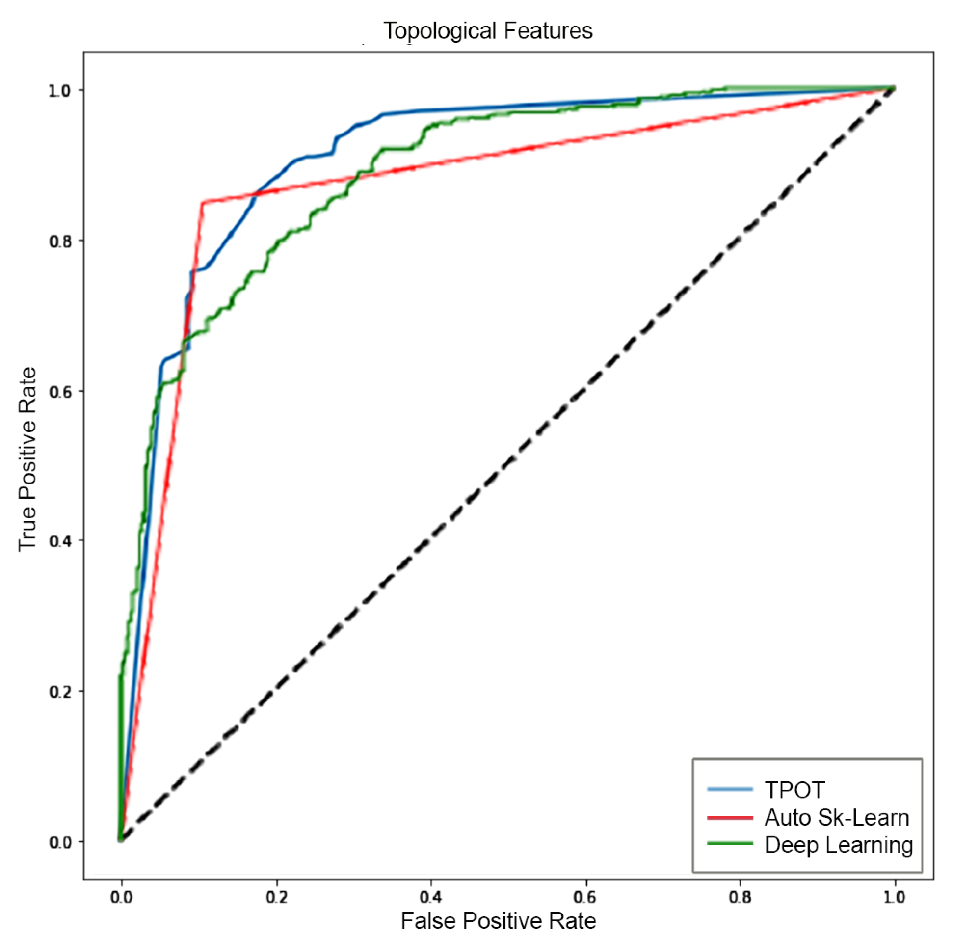
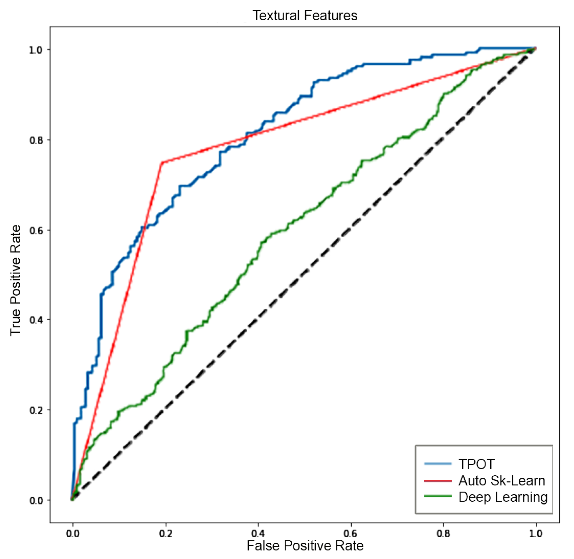
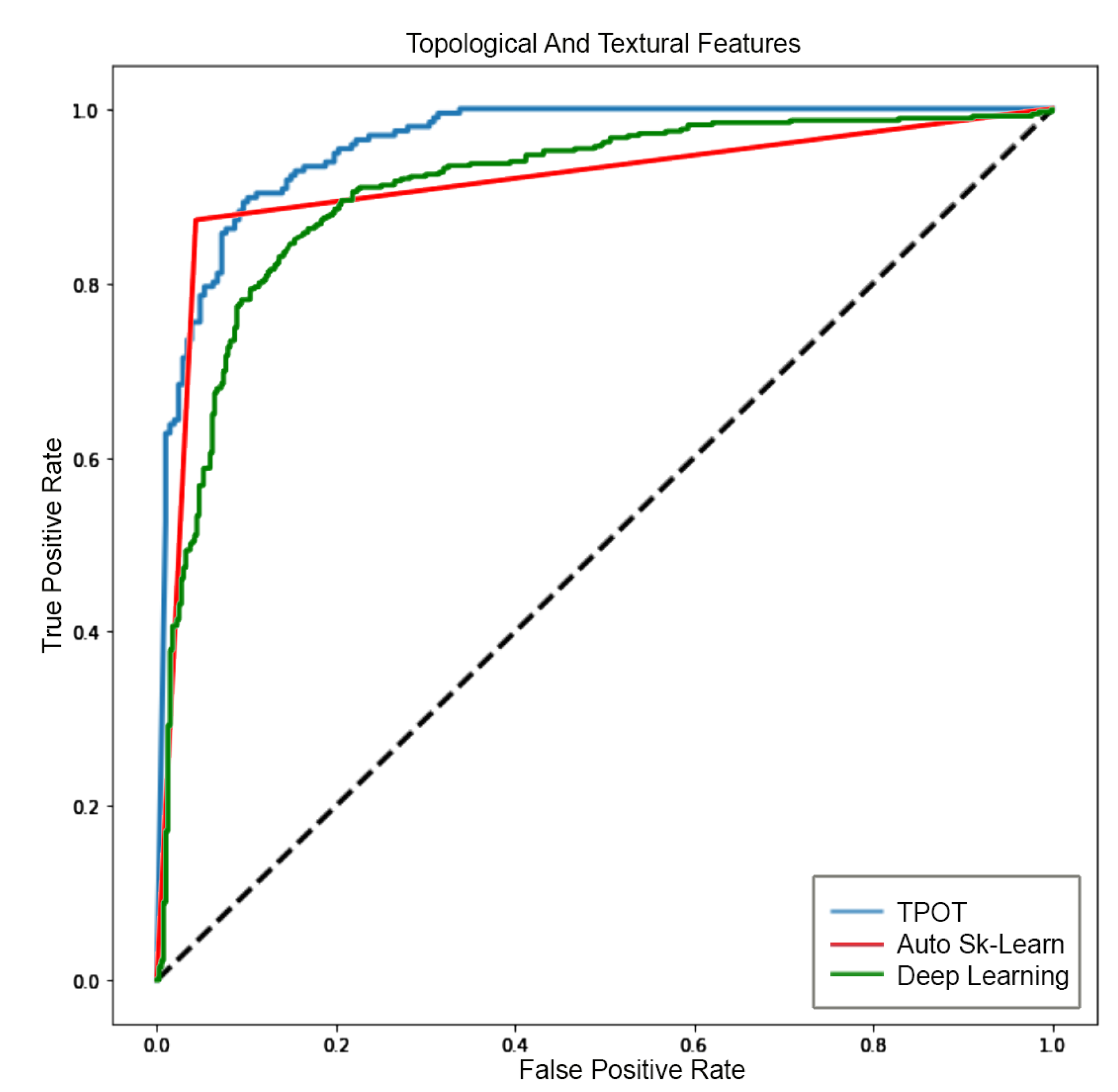
4.3. Analysis 3: GBM Classification
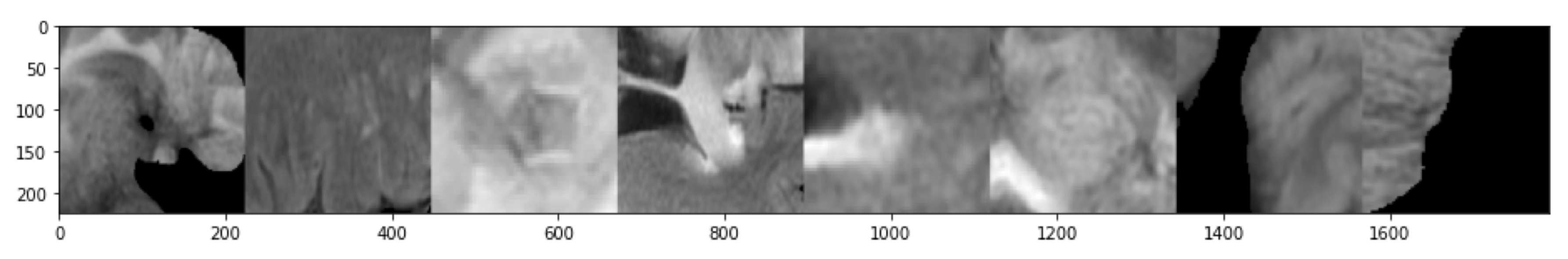
- 2D GLCM features and topological features were calculated with a sliding patch approach in the segmented ROI. The size of the patch is .
- In order to identify discriminating features, the same feature calculations were also performed in the contralateral (healthy) ROIs.
- Each sliding patch was labeled as healthy or ill according to the class of its ROI. Each patch was also stored for future analysis.
- Features selection.
- The dataset is randomly divided into training and testing subsets that contain the 70% and 30% of samples, respectively.
- The training set is used for training a machine learning classifier. For the sake of completeness, during training we adopted a k-fold cross validation standard procedure [71] (https://machinelearningmastery.com/difference-test-validation-datasets/) with .
- Splitting, training and testing procedures were executed multiple times by using different set of features—only topological features or only GLCM features or topological plus GLCM features.
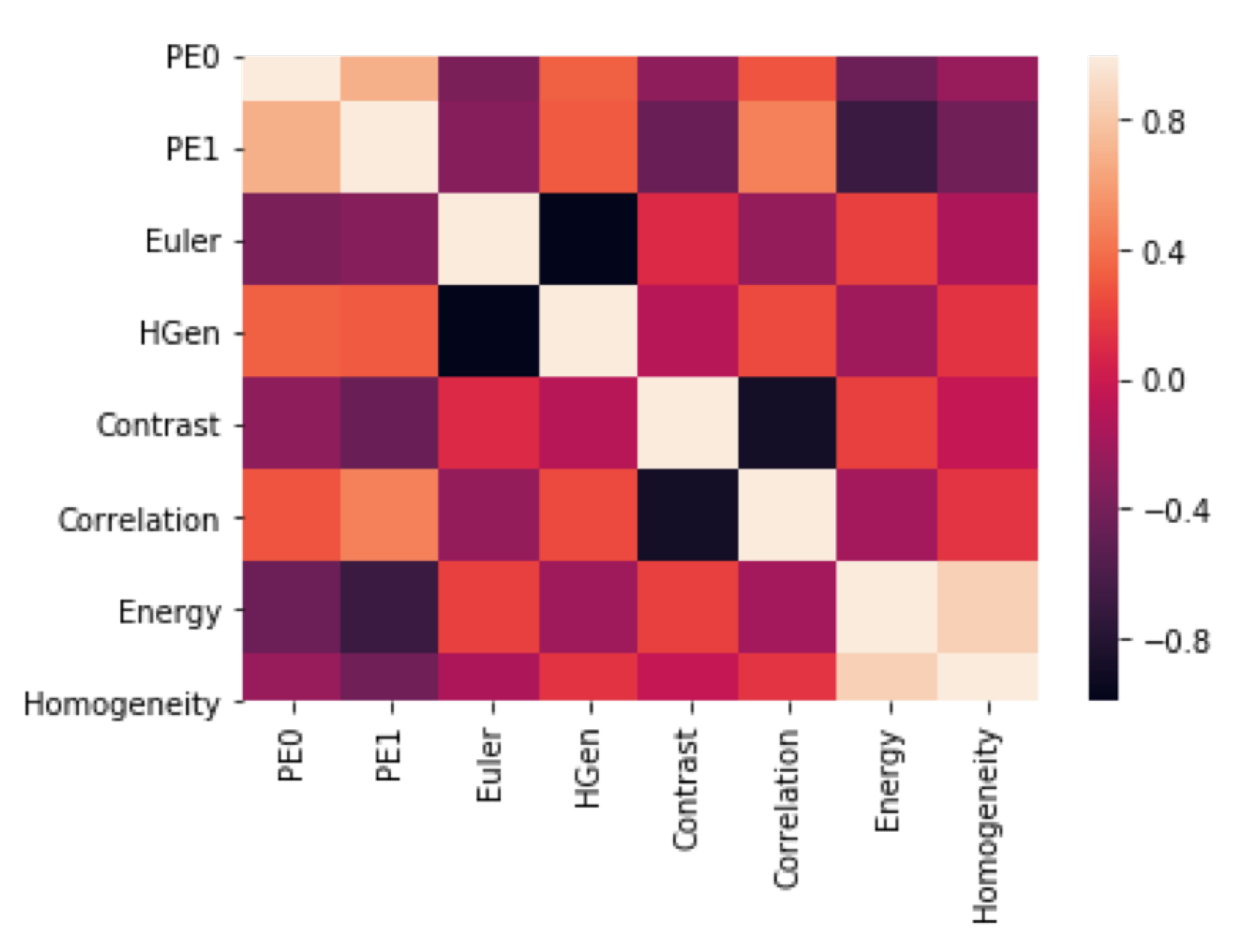
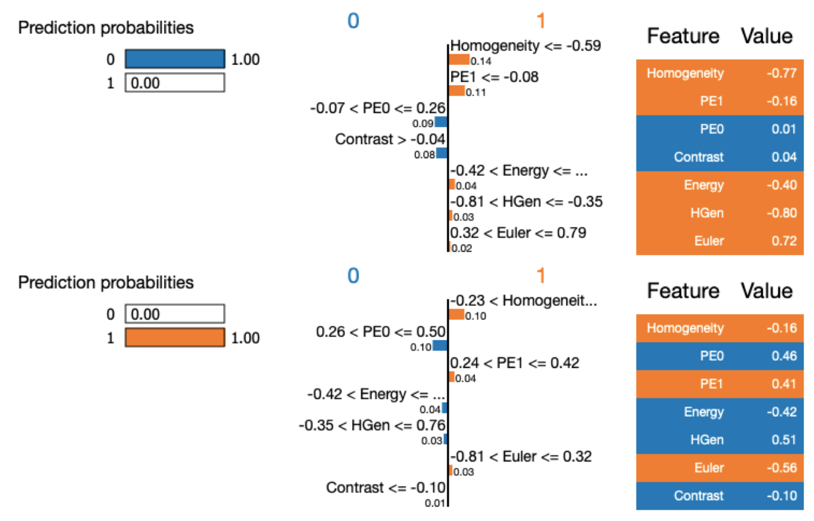
- Classifier behavior is debugged by tools from information theory. This allows to understand feature relevance and to understand what are the numerical input characteristics related to the classification verdict. Specifically, we have used Skater and Lime algorithms [72] (https://www.oreilly.com/ideas/interpreting-predictive-models-with-skater-unboxing-model-opacity).
4.3.1. Feature Selection
4.3.2. Machine Learning Algorithm Selection
4.3.3. Deep Learning Approach on Numerical Features
4.3.4. Gbm Classification—Deep Learning Approach on Patches
5. Results
5.1. Analysis 1: Topological Data Analysis of a Simplified 2D Tumor Growth Mathematical Model
5.2. Analysis 2: Topological Data Analysis of tumor Progression
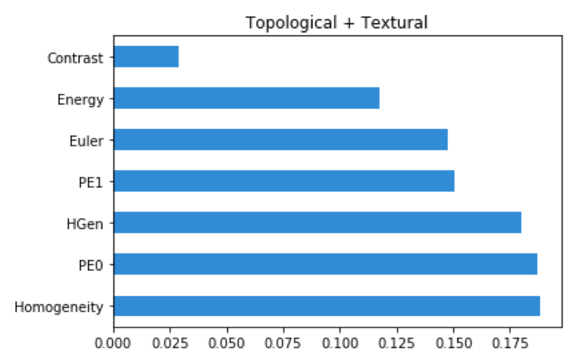
5.3. Analysis 3: GBM Classification on FLAIR
Machine Learning Classification Interpretation
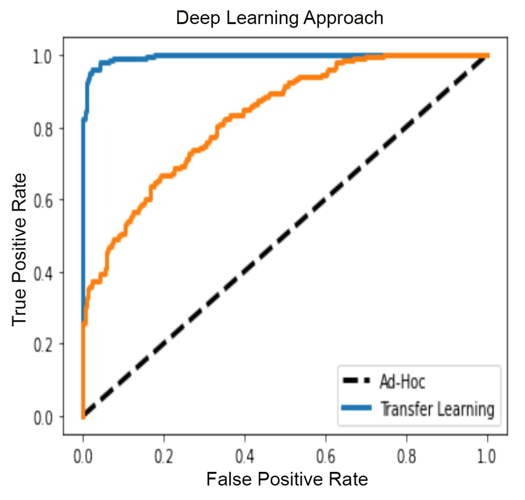
5.4. GBM Classification with Deep Learning
6. Discussion
Author Contributions
Funding
Acknowledgments
Conflicts of Interest
Abbreviations
| GBM | Glioblastomas multiforme |
| GLCM | grey Level Co-occurrence Matrix |
| TDA | Topological Data Analysis |
| MRI | Magnetic Resonance Image |
| FLAIR | Fluid-attenuated inversion recovery |
| MD | Medical Doctor |
References
- Batash, R.; Asna, N.; Schaffer, P.; Francis, N.; Schaffer, M. Glioblastoma multiforme, diagnosis and treatment; recent literature review. Curr. Med. Chem. 2017, 24, 3002–3009. [Google Scholar] [CrossRef] [PubMed]
- Weller, M.; Van den Bent, M.; Hopkins, K.; Tonn, J.; Stupp, R.; Falini, A.; Cohen-Jonathan-Moyal, E.; Frappaz, D.; Henriksson, R.; Balana, C.; et al. European Association for Neuro-Oncology (EANO) Task Force on Malignant Glioma. EANO guideline for the diagnosis and treatment of anaplastic gliomas and glioblastoma. Lancet Oncol. 2014, 15, e395–e403. [Google Scholar] [CrossRef]
- Kuhnt, D.; Becker, A.; Ganslandt, O.; Bauer, M.; Buchfelder, M.; Nimsky, C. Correlation of the extent of tumor volume resection and patient survival in surgery of glioblastoma multiforme with high-field intraoperative MRI guidance. Neuro-Oncology 2011, 13, 1339–1348. [Google Scholar] [CrossRef] [PubMed]
- Kubben, P.L.; ter Meulen, K.J.; Schijns, O.E.M.G.; ter Laak-Poort, M.P.; van Overbeeke, J.J.; van Santbrink, H. Intraoperative MRI-guided resection of glioblastoma multiforme: A systematic review. Lancet Oncol. 2011, 12, 1062–1070. [Google Scholar] [CrossRef]
- Majós, C.; Cos, M.; Castañer, S.; Gil, M.; Plans, G.; Lucas, A.; Bruna, J.; Aguilera, C. Early post-operative magnetic resonance imaging in glioblastoma: correlation among radiological findings and overall survival in 60 patients. Eur. Radiol. 2016, 26, 1048–1055. [Google Scholar] [CrossRef] [PubMed]
- Damadian, R. Tumor detection by nuclear magnetic resonance. Science 1971, 171, 1151–1153. [Google Scholar] [CrossRef]
- Castellano, A.; Donativi, M.; Rudà, R.; De Nunzio, G.; Riva, M.; Iadanza, A.; Bertero, L.; Rucco, M.; Bello, L.; Soffietti, R.; et al. Evaluation of low-grade glioma structural changes after chemotherapy using DTI-based histogram analysis and functional diffusion maps. Eur. Radiol. 2016, 26, 1263–1273. [Google Scholar] [CrossRef]
- Castellano, G.; Bonilha, L.; Li, L.; Cendes, F. Texture analysis of medical images. Clin. Radiol. 2004, 59, 1061–1069. [Google Scholar] [CrossRef]
- Remondino, F.; El-Hakim, S. Image-based 3D modelling: A review. Photogramm. Rec. 2006, 21, 269–291. [Google Scholar] [CrossRef]
- Schad, L.R.; Blüml, S.; Zuna, I. MR tissue characterization of intracranial tumors by means of texture analysis. Magn. Reson. Imaging 1993, 11, 889–896. [Google Scholar] [CrossRef]
- Zhao, Z.; Yang, G.; Lin, Y.; Pang, H.; Wang, M. Automated glioma detection and segmentation using graphical models. PLoS ONE 2018, 13, e0200745. [Google Scholar] [CrossRef] [PubMed]
- Wu, Y.; Zhao, Z.; Wu, W.; Lin, Y.; Wang, M. Automatic glioma segmentation based on adaptive superpixel. BMC Med. Imaging 2019, 19, 73. [Google Scholar] [CrossRef]
- Shivhare, S.N.; Kumar, N. Brain tumor detection using manifold ranking in flair mri. In Proceedings of ICETIT 2019; Springer: Berlin/Heidelberg, Germany, 2020; pp. 292–305. [Google Scholar]
- Soltaninejad, M.; Yang, G.; Lambrou, T.; Allinson, N.; Jones, T.L.; Barrick, T.R.; Howe, F.A.; Ye, X. Automated brain tumor detection and segmentation using superpixel-based extremely randomized trees in FLAIR MRI. Int. J. Comput. Assist. Radiol. Surg. 2017, 12, 183–203. [Google Scholar] [CrossRef] [PubMed]
- Korfiatis, P.; Kline, T.L.; Erickson, B.J. Automated segmentation of hyperintense regions in FLAIR MRI using deep learning. Tomography 2016, 2, 334. [Google Scholar] [PubMed]
- Lorenzo, P.R.; Nalepa, J.; Bobek-Billewicz, B.; Wawrzyniak, P.; Mrukwa, G.; Kawulok, M.; Ulrych, P.; Hayball, M.P. Segmenting brain tumors from FLAIR MRI using fully convolutional neural networks. Comput. Methods Programs Biomed. 2019, 176, 135–148. [Google Scholar] [CrossRef] [PubMed]
- Kleesiek, J.; Urban, G.; Hubert, A.; Schwarz, D.; Maier-Hein, K.; Bendszus, M.; Biller, A. Deep MRI brain extraction: A 3D convolutional neural network for skull stripping. NeuroImage 2016, 129, 460–469. [Google Scholar] [CrossRef]
- Galdames, F.J.; Jaillet, F.; Perez, C.A. An accurate skull stripping method based on simplex meshes and histogram analysis for magnetic resonance images. J. Neurosci. Methods 2012, 206, 103–119. [Google Scholar] [CrossRef]
- Chaddad, A.; Kucharczyk, M.J.; Daniel, P.; Sabri, S.; Jean-Claude, B.J.; Niazi, T.; Abdulkarim, B. Radiomics in glioblastoma: Current status and challenges facing clinical implementation. Front. Oncol. 2019, 9, 374. [Google Scholar] [CrossRef]
- Bellomo, N.; Preziosi, L. Modelling and mathematical problems related to tumor evolution and its interaction with the immune system. Math. Comput. Model. 2000, 32, 413–452. [Google Scholar] [CrossRef]
- Michel, T.; Fehrenbach, J.; Lobjois, V.; Laurent, J.; Gomes, A.; Colin, T.; Poignard, C. Mathematical modeling of the proliferation gradient in multicellular tumor spheroids. J. Theor. Biol. 2018, 458, 133–147. [Google Scholar] [CrossRef]
- Unsal, S.; Acar, A.; Itik, M.; Kabatas, A.; Gedikli, O.; Ozdemir, F.; Turhan, K. Personalized Tumor Growth Prediction with Multiscale Tumor Modeling. bioRxiv 2019, 510172. [Google Scholar] [CrossRef]
- Hatcher, A. Algebraic Topology; Cambridge University Press: Cambridge, UK, 2002. [Google Scholar]
- Munkres, J.R. Elements of Algebraic Topology; Addison-Wesley: Reading, MA, USA, 1984; Volume 2. [Google Scholar]
- Carlsson, G. Topology and data. Bull. Am. Math. Soc. 2009, 46, 255–308. [Google Scholar] [CrossRef]
- Zomorodian, A. Topological data analysis. In Advances in Applied and Computational Topology, Proceedings of the Symposia in Applied Mathematics, New Orleans, LA, USA, 4–5 January 2011; Zomorodian, A.J., Ed.; American Mathematical Society: Providence, RI, USA, 2012; Volume 70, pp. 1–39. [Google Scholar]
- Edelsbrunner, H.; Harer, J. Persistent Homology—A Survey. Contemp. Math. 2008, 453, 257–282. [Google Scholar]
- Rucco, M.; Mamuye, A.L.; Piangerelli, M.; Quadrini, M.; Tesei, L.; Merelli, E. Survey of TOPDRIM applications of topological data analysis. In CEUR Workshop Proceedings; RWTH Aachen University: Aachen, Germany, 2016; Volume 1748, p. 1814. [Google Scholar]
- Atienza, N.; Gonzalez-Diaz, R.; Rucco, M. Persistent entropy for separating topological features from noise in vietoris-rips complexes. J. Intell. Inf. Syst. 2019, 52, 637–655. [Google Scholar] [CrossRef]
- Jimenez, M.J.; Rucco, M.; Vicente-Munuera, P.; Gómez-Gálvez, P.; Escudero, L.M. Topological data analysis for self-organization of biological tissues. In International Workshop on Combinatorial Image Analysis; Springer: Berlin/Heidelberg, Germany, 2017; pp. 229–242. [Google Scholar]
- Piangerelli, M.; Rucco, M.; Tesei, L.; Merelli, E. Topological classifier for detecting the emergence of epileptic seizures. BMC Res. Notes 2018, 11, 392. [Google Scholar] [CrossRef]
- Oyama, A.; Hiraoka, Y.; Obayashi, I.; Saikawa, Y.; Furui, S.; Shiraishi, K.; Kumagai, S.; Hayashi, T.; Kotoku, J. Hepatic tumor classification using texture and topology analysis of non-contrast-enhanced three-dimensional T1-weighted MR images with a radiomics approach. Sci. Rep. 2019, 9, 8764. [Google Scholar] [CrossRef]
- Gholizadeh, S.; Zadrozny, W. A Short Survey of Topological Data Analysis in Time Series and Systems Analysis. arXiv 2018, arXiv:1809.10745. [Google Scholar]
- Myers, A.; Munch, E.; Khasawneh, F.A. Persistent homology of complex networks for dynamic state detection. Phys. Rev. E 2019, 100, 022314. [Google Scholar] [CrossRef]
- Cámara, P.G. Topological methods for genomics: Present and future directions. Curr. Opin. Syst. Biol. 2017, 1, 95–101. [Google Scholar] [CrossRef]
- Lambin, P.; Leijenaar, R.T.; Deist, T.M.; Peerlings, J.; De Jong, E.E.; Van Timmeren, J.; Sanduleanu, S.; Larue, R.T.; Even, A.J.; Jochems, A.; et al. Radiomics: The bridge between medical imaging and personalized medicine. Nat. Rev. Clin. Oncol. 2017, 14, 749. [Google Scholar] [CrossRef]
- Fave, X.; Zhang, L.; Yang, J.; Mackin, D.; Balter, P.; Gomez, D.; Followill, D.; Jones, A.K.; Stingo, F.; Liao, Z.; et al. Delta-radiomics features for the prediction of patient outcomes in non–small cell lung cancer. Sci. Rep. 2017, 7, 1–11. [Google Scholar] [CrossRef] [PubMed]
- Crawford, L.; Monod, A.; Chen, A.X.; Mukherjee, S.; Rabadán, R. Predicting clinical outcomes in glioblastoma: An application of topological and functional data analysis. J. Am. Stat. Assoc. 2019, 1–12. [Google Scholar] [CrossRef]
- Joshi, M.; Joshi, D. A survey of Topological Data Analysis Methods for Big Data in Healthcare Intelligence. Int. J. Appl. Eng. Res. 2019, 14, 584–588. [Google Scholar]
- Thai, M.T.; Wu, W.; Xiong, H. Big Data in Complex and Social Networks; CRC Press: Boca Raton, FL, USA, 2016. [Google Scholar]
- Petri, G.; Scolamiero, M.; Donato, I.; Vaccarino, F. Topological strata of weighted complex networks. PLoS ONE 2013, 8, e66506. [Google Scholar] [CrossRef] [PubMed]
- Zhang, Q.; Yang, L.T.; Chen, Z.; Li, P. A survey on deep learning for big data. Inf. Fusion 2018, 42, 146–157. [Google Scholar] [CrossRef]
- Qiu, J.; Wu, Q.; Ding, G.; Xu, Y.; Feng, S. A survey of machine learning for big data processing. EURASIP J. Adv. Signal Process. 2016, 2016, 67. [Google Scholar] [CrossRef]
- Sherratt, J.A.; Chaplain, M.A. A new mathematical model for avascular tumor growth. J. Math. Biol. 2001, 43, 291–312. [Google Scholar] [CrossRef]
- Böttger, K.; Hatzikirou, H.; Chauviere, A.; Deutsch, A. Investigation of the migration/proliferation dichotomy and its impact on avascular glioma invasion. Math. Model. Nat. Phenom. 2012, 7, 105–135. [Google Scholar] [CrossRef][Green Version]
- Stein, A.M.; Demuth, T.; Mobley, D.; Berens, M.; Sander, L.M. A mathematical model of glioblastoma tumor spheroid invasion in a three-dimensional in vitro experiment. Biophys. J. 2007, 92, 356–365. [Google Scholar] [CrossRef]
- Ang, K.C. Analysis of a tumor growth model with MATLAB. Available online: http://hdl.handle.net/10497/14941 (accessed on 1 May 2020).
- Clark, K.; Vendt, B.; Smith, K.; Freymann, J.; Kirby, J.; Koppel, P.; Moore, S.; Phillips, S.; Maffitt, D.; Pringle, M.; et al. The Cancer Imaging Archive (TCIA): Maintaining and operating a public information repository. J. Digit. Imaging 2013, 26, 1045–1057. [Google Scholar] [CrossRef]
- Schmainda, K.; Prah, M. Data from Brain Tumor Progression. The Cancer Imaging Archive. Available online: http://doi.org/10.7937/K9/TCIA.2018.15quzvnb (accessed on 10 May 2020).
- Ellingson, B.; Malkin, M.; Rand, S.; Bedekar, D.; Schmainda, K. Functional diffusion maps applied to FLAIR abnormal areas are valuable for the clinical monitoring of recurrent brain tumors. Proc. Intl. Soc. Mag. Reson Med. 2009, 17, 285. [Google Scholar]
- Schmainda, K.M.; Prah, M.A.; Rand, S.D.; Liu, Y.; Logan, B.; Muzi, M.; Rane, S.D.; Da, X.; Yen, Y.F.; Kalpathy-Cramer, J.; et al. Multi-site Concordance of DSC-MRI Analysis for Brain tumors: Results of a NCI Quantitative Imaging network collaborative project. AJNR. Am. J. Neuroradiol. 2018, 39, 1008. [Google Scholar] [CrossRef] [PubMed]
- Lipková, J.; Angelikopoulos, P.; Wu, S.; Alberts, E.; Wiestler, B.; Diehl, C.; Preibisch, C.; Pyka, T.; Combs, S.E.; Hadjidoukas, P.; et al. Personalized Radiotherapy Design for Glioblastoma: Integrating Mathematical Tumor Models, Multimodal Scans, and Bayesian Inference. IEEE Trans. Med Imaging 2019, 38, 1875–1884. [Google Scholar] [CrossRef] [PubMed]
- Edelsbrunner, H.; Harer, J. Computational Topology: An Introduction; American Mathematical Society: Providence, RI, USA, 2010. [Google Scholar]
- Adams, H.; Tausz, A.; Vejdemo-Johansson, M. JavaPlex: A research software package for persistent (co) homology. In International Congress on Mathematical Software; Springer: Berlin/Heidelberg, Germany, 2014; pp. 129–136. [Google Scholar]
- Otter, N.; Porter, M.A.; Tillmann, U.; Grindrod, P.; Harrington, H.A. A roadmap for the computation of persistent homology. EPJ Data Sci. 2017, 6, 17. [Google Scholar] [CrossRef]
- Chintakunta, H.; Gentimis, T.; Gonzalez-Diaz, R.; Jimenez, M.J.; Krim, H. An entropy-based persistence barcode. Pattern Recognit. 2015, 48, 391–401. [Google Scholar] [CrossRef]
- Rucco, M.; Castiglione, F.; Merelli, E.; Pettini, M. Characterisation of the idiotypic immune network through persistent entropy. In Proceedings of ECCS 2014; Springer: Berlin/Heidelberg, Germany, 2016; pp. 117–128. [Google Scholar]
- Rucco, M.; Gonzalez-Diaz, R.; Jimenez, M.J.; Atienza, N.; Cristalli, C.; Concettoni, E.; Ferrante, A.; Merelli, E. A new topological entropy-based approach for measuring similarities among piecewise linear functions. Signal Process. 2017, 134, 130–138. [Google Scholar] [CrossRef]
- Ghrist, R. Barcodes: The persistent topology of data. Bull. Am. Math. Soc. 2008, 45, 61–75. [Google Scholar] [CrossRef]
- Obayashi, I. Volume-optimal cycle: Tightest representative cycle of a generator in persistent homology. SIAM J. Appl. Algebra Geom. 2018, 2, 508–534. [Google Scholar] [CrossRef]
- Chaddad, A.; Zinn, P.O.; Colen, R.R. Radiomics texture feature extraction for characterizing GBM phenotypes using GLCM. In Proceedings of the 2015 IEEE 12th International Symposium on Biomedical Imaging (ISBI), Brooklyn Bridge, NY, USA, 16–19 April 2015; pp. 84–87. [Google Scholar]
- Haralick, R.M.; Shanmugam, K.; Dinstein, I.H. Textural features for image classification. IEEE Trans. Syst. Man Cybern. 1973, 3, 610–621. [Google Scholar] [CrossRef]
- Tralie, C.; Saul, N.; Bar-On, R. Ripser.py: A Lean Persistent Homology Library for Python. J. Open Source Softw. 2018, 3, 925. [Google Scholar] [CrossRef]
- Van der Walt, S.; Schönberger, J.L.; Nunez-Iglesias, J.; Boulogne, F.; Warner, J.D.; Yager, N.; Gouillart, E.; Yu, T. scikit-image: Image processing in Python. PeerJ 2014, 2, e453. [Google Scholar] [CrossRef] [PubMed]
- Hajian-Tilaki, K. Receiver operating characteristic (ROC) curve analysis for medical diagnostic test evaluation. Casp. J. Intern. Med. 2013, 4, 627. [Google Scholar]
- Wilkerson, A.C.; Chintakunta, H.; Krim, H. Computing persistent features in big data: A distributed dimension reduction approach. In Proceedings of the 2014 IEEE International Conference on Acoustics, Speech and Signal Processing (ICASSP), Florence, Italy, 4–9 May 2014; pp. 11–15. [Google Scholar]
- Lewis, R.; Morozov, D. Parallel computation of persistent homology using the blowup complex. In Proceedings of the 27th ACM Symposium on Parallelism in Algorithms and Architectures, Portland, OR, USA, 24–26 June 2015; pp. 323–331. [Google Scholar]
- Gunther, D.; Reininghaus, J.; Hotz, I.; Wagner, H. Memory-efficient computation of persistent homology for 3d images using discrete Morse theory. In Proceedings of the 2011 24th SIBGRAPI Conference on Graphics, Patterns and Images, Maceio, Brazil, 28–31 August 2011; pp. 25–32. [Google Scholar]
- Clausi, D.A. An analysis of co-occurrence texture statistics as a function of grey level quantization. Can. J. Remote Sens. 2002, 28, 45–62. [Google Scholar] [CrossRef]
- Kearns, M.J. The Computational Complexity of Machine Learning; MIT Press: Cambridge, MA, USA, 1990. [Google Scholar]
- Wong, T.T. Performance evaluation of classification algorithms by k-fold and leave-one-out cross validation. Pattern Recognit. 2015, 48, 2839–2846. [Google Scholar] [CrossRef]
- Wei, P.; Lu, Z.; Song, J. Variable importance analysis: A comprehensive review. Reliab. Eng. Syst. Saf. 2015, 142, 399–432. [Google Scholar] [CrossRef]
- Feurer, M.; Klein, A.; Eggensperger, K.; Springenberg, J.; Blum, M.; Hutter, F. Efficient and Robust Automated Machine Learning. In Advances in Neural Information Processing Systems 28; Cortes, C., Lawrence, N.D., Lee, D.D., Sugiyama, M., Garnett, R., Eds.; Curran Associates, Inc.: Red Hook, NY, USA, 2015; pp. 2962–2970. [Google Scholar]
- Olson, R.S.; Moore, J.H. TPOT: A tree-based pipeline optimization tool for automating machine learning. In Automated Machine Learning; Springer: Berlin/Heidelberg, Germany, 2019; pp. 151–160. [Google Scholar]
- Zhao, D.; Zhu, D.; Lu, J.; Luo, Y.; Zhang, G. Synthetic medical images using F&BGAN for improved lung nodules classification by multi-scale VGG16. Symmetry 2018, 10, 519. [Google Scholar]
- Ahlgren, F.; Thern, M. Auto Machine Learning for predicting Ship Fuel Consumption. In Proceedings of the ECOS 2018—The 31st International Conference on Efficiency, Cost, Optimization, Simulation and Environmental Impact of Energy Systems, Guimarães, Portugal, 17–21 June 2018. [Google Scholar]
- Stummer, W.; Pichlmeier, U.; Meinel, T.; Wiestler, O.D.; Zanella, F.; Reulen, H.J.; ALA-Glioma Study Group. Fluorescence-guided surgery with 5-aminolevulinic acid for resection of malignant glioma: A randomised controlled multicentre phase III trial. Lancet Oncol. 2006, 7, 392–401. [Google Scholar] [CrossRef]
- Hart, M.G.; Grant, R.; Garside, R.; Rogers, G.; Somerville, M.; Stein, K. Chemotherapeutic wafers for high grade glioma. In Cochrane Database of Systematic Reviews; John Wiley & Sons: Hoboken, NJ, USA, 2008. [Google Scholar]
- Colombo, M.C.; Giverso, C.; Faggiano, E.; Boffano, C.; Acerbi, F.; Ciarletta, P. Towards the personalized treatment of glioblastoma: Integrating patient-specific clinical data in a continuous mechanical model. PLoS ONE 2015, 10. [Google Scholar] [CrossRef]
- Ion-Mărgineanu, A.; Van Cauter, S.; Sima, D.M.; Maes, F.; Sunaert, S.; Himmelreich, U.; Van Huffel, S. Classifying glioblastoma multiforme follow-up progressive vs. responsive forms using multi-parametric MRI features. Front. Neurosci. 2017, 10, 615. [Google Scholar] [CrossRef] [PubMed][Green Version]
- Lachinov, D.; Vasiliev, E.; Turlapov, V. Glioma segmentation with cascaded UNet. In International MICCAI Brainlesion Workshop; Springer: Berlin/Heidelberg, Germany, 2018; pp. 189–198. [Google Scholar]
- Shaver, M.M.; Kohanteb, P.A.; Chiou, C.; Bardis, M.D.; Chantaduly, C.; Bota, D.; Filippi, C.G.; Weinberg, B.; Grinband, J.; Chow, D.S.; et al. Optimizing Neuro-Oncology Imaging: A Review of Deep Learning Approaches for Glioma Imaging. Cancers 2019, 11, 829. [Google Scholar] [CrossRef]
- Ronneberger, O.; Fischer, P.; Brox, T. U-net: Convolutional networks for biomedical image segmentation. In International Conference on Medical Image Computing and Computer-Assisted Intervention; Springer: Berlin/Heidelberg, Germany, 2015; pp. 234–241. [Google Scholar]


| Topological Statistics | ||||
|---|---|---|---|---|
| Pre | Post | t-Test | p-Value | |
| Euler Characteristics | −773.94 +/− 62.98 | −830.31 +/− 74.55 | 1.84 | 0.06 |
| Persistent Entropy H0 | 0.44 +/− 0.23 | 0.51 +/− 0.24 | −6.79 | 0.01 |
| Persistent Entropy H1 | 0.70 +/− 0.15 | 0.70 +/− 0.16 | −0.29 | 0.77 |
| Generator Entropy H1 | 0.30 +/− 0.26 | 0.28 +/− 0.27 | 1.68 | 0.09 |
| Topological Features | ||||||
|---|---|---|---|---|---|---|
| TPOT | Auto Sci-Kit Learn | Deep Learning | ||||
| Metric | Train | Test | Train | Test | Train | Test |
| Accuracy | 0.89 | 0.84 | 0.97 | 0.87 | 0.82 | 0.79 |
| Precision | 0.88 | 0.83 | 0.97 | 0.88 | 0.90 | 0.91 |
| Recall | 0.88 | 0.84 | 0.96 | 0.84 | 0.72 | 0.67 |
| Misclassification rate | 0.10 | 0.16 | 0.03 | 0.13 | 0.17 | 0.20 |
| F1 | 0.89 | 0.83 | 0.97 | 0.88 | 0.80 | 0.77 |
| AUC | 0.89 | 0.89 | 0.97 | 0.87 | 0.82 | 0.79 |
| Topological Features | ||||||
|---|---|---|---|---|---|---|
| TPOT | Auto Sci-Kit Learn | Deep Learning | ||||
| Metric | Train | Test | Train | Test | Train | Test |
| Accuracy | 1.00 | 0.71 | 0.93 | 0.77 | 0.60 | 0.58 |
| Precision | 1.00 | 0.70 | 0.94 | 0.78 | 0.61 | 0.60 |
| Recall | 1.00 | 0.71 | 0.92 | 0.74 | 0.51 | 0.51 |
| Misclassification rate | 0.00 | 0.28 | 0.07 | 0.23 | 0.40 | 0.42 |
| F1 | 1.00 | 0.71 | 0.93 | 0.76 | 0.56 | 0.55 |
| AUC | 1.00 | 0.81 | 0.93 | 0.77 | 0.60 | 0.57 |
| Topological Features | ||||||
|---|---|---|---|---|---|---|
| TPOT | Auto Sci-Kit Learn | Deep Learning | ||||
| Metric | Train | Test | Train | Test | Train | Test |
| Accuracy | 0.96 | 0.89 | 0.98 | 0.92 | 0.90 | 0.89 |
| Precision | 0.96 | 0.89 | 0.99 | 0.95 | 0.87 | 0.85 |
| Recall | 0.95 | 0.89 | 0.97 | 0.87 | 0.93 | 0.84 |
| Misclassification rate | 0.04 | 0.10 | 0.02 | 0.08 | 0.09 | 0.15 |
| F1 | 0.96 | 0.89 | 0.98 | 0.91 | 0.90 | 0.84 |
| AUC | 0.99 | 0.96 | 0.98 | 0.91 | 0.90 | 0.84 |
| Deep Learning on Patches | ||||
|---|---|---|---|---|
| VGG16 Transfer Learning | Ad-Hoc | |||
| Metric | Train | Test | Train | Test |
| Accuracy | 0.99 | 0.97 | 0.74 | 0.75 |
| Precision | 1.00 | 0.99 | 0.67 | 0.66 |
| Recall | 0.98 | 0.95 | 0.97 | 0.95 |
| Misclassification rate | 0.01 | 0.03 | 0.26 | 0.25 |
| F1 | 0.99 | 0.97 | 0.79 | 0.78 |
| AUC | 0.99 | 0.97 | 0.74 | 0.77 |
© 2020 by the authors. Licensee MDPI, Basel, Switzerland. This article is an open access article distributed under the terms and conditions of the Creative Commons Attribution (CC BY) license (http://creativecommons.org/licenses/by/4.0/).
Share and Cite
Rucco, M.; Viticchi, G.; Falsetti, L. Towards Personalized Diagnosis of Glioblastoma in Fluid-Attenuated Inversion Recovery (FLAIR) by Topological Interpretable Machine Learning. Mathematics 2020, 8, 770. https://doi.org/10.3390/math8050770
Rucco M, Viticchi G, Falsetti L. Towards Personalized Diagnosis of Glioblastoma in Fluid-Attenuated Inversion Recovery (FLAIR) by Topological Interpretable Machine Learning. Mathematics. 2020; 8(5):770. https://doi.org/10.3390/math8050770
Chicago/Turabian StyleRucco, Matteo, Giovanna Viticchi, and Lorenzo Falsetti. 2020. "Towards Personalized Diagnosis of Glioblastoma in Fluid-Attenuated Inversion Recovery (FLAIR) by Topological Interpretable Machine Learning" Mathematics 8, no. 5: 770. https://doi.org/10.3390/math8050770
APA StyleRucco, M., Viticchi, G., & Falsetti, L. (2020). Towards Personalized Diagnosis of Glioblastoma in Fluid-Attenuated Inversion Recovery (FLAIR) by Topological Interpretable Machine Learning. Mathematics, 8(5), 770. https://doi.org/10.3390/math8050770