Transferable Architecture for Segmenting Maxillary Sinuses on Texture-Enhanced Occipitomental View Radiographs

Abstract

Maxillary sinuses are the most prevalent locations for paranasal infections on both children and adults. Common diagnostic material for this particular disease is through the screening of occipitomental-view skull radiography (SXR). With the growing cases on paranasal infections, expediting the diagnosis has become an important innovation aspect that could be addressed through the development of a computer-aided diagnosis system. As the preliminary stage of the development, an automatic segmentation over the maxillary sinuses is required to be developed. This study presents a computer-aided detection (CAD) module that segments maxillary sinuses from a plain SXR that has been preprocessed through the novel texture-based morphological analysis (ToMA). Later, the network model from the Transferable Fully Convolutional Network (T-FCN) performs pixel-wise segmentation of the maxillary sinuses. T-FCN is designed to be trained with multiple learning stages, which enables re-utilization of network weights to be adjusted based on newer dataset. According to the experiments, the proposed system achieved segmentation accuracy at 85.70%, with 50% faster learning time.

1. Introduction

Maxillary sinusitis is the most common infection-type paranasal disease associated with both adults and children [1,2], which could be diagnosed through radiography screening. The appropriate modality for radiography imaging might either be plain radiography (X-ray) or computed tomography (CT). The coronal sinus CT (SCT) provides the gold standard for diagnosing maxillary sinusitis because of its superiority in image quality compared to the occipitomental-view X-ray (SXR) [3] that often suffers from texture ambiguities caused by the overlapping structures or because of low contrast ratio [4].

On the other hand, the effective radiation dose of SXR yields around 0.1 mSv, which is 20 times smaller than the effective radiation dose of SCT [5], thus making the SXR a safer approach for periodical diagnosis. Despite the trade-off between image quality and radiation dose, SXR images might be utilized to diagnose maxillary sinusitis if the perceived quality achieves sufficient conditions [6] that could be carried out using an enhancement technique.

Few studies [7,8,9,10,11] have developed histogram-based image enhancement for medical images that remaps the pixel distributions to have higher contrast ratio. Although final contrast ratio might improve, there are few drawbacks, which have decimated the merits of prior arts, including noise amplification [7], generation of undesired texture [8], and inferior improvement on contrast ratio over the soft tissues [7,8]. These issues are aimed to be addressed through the first part of the proposed framework, image enhancement. In Reference [9], they proposed image enhancement for medical images based on world cup optimization (WCO) algorithm utilizing gamma correction method to enhance and highlight the information in medical images. However, predicting a suitable value for gamma is still challenging task that results in unnecessary artifacts and blurry areas in the image.

Medical observation over the maxillary sinuses by medical experts for any apparent symptoms, such as cysts or mucous thickening, on an SXR image is also an essential aspect for identifying the inflammatory condition of the subject’s maxillary sinuses. However, the insufficient distributions of medical professionals in the field have raised the contingency for developing an automated detection system to semantically segments the maxillary sinuses. The segmentation result could either assist an amateur radiologist(s) to perform observation or as an input for the possible development of fully automatic diagnosis system [12].

Image segmentation remains an arduous task for high-level object understanding [13]. Currently, most prior arts focus on providing a segmentation algorithm using deep learning solution for CT images [12,14]. The work presented in Reference [15] proposed a correction learning scheme that processes the segmented lesion on a cropped mammography from superpixel-based technique to be improved using block-based boundary correction. Despite the simplicity of Reference [15], erroneous segmentation does not modify any network’s weight, while it also may not applicable for SXRs with many arduous textures.

One of the state-of-the-art options is a Fully Convolutional Network (FCN) that is comprised of convolutional (encoder) and deconvolutional (decoder) networks to extract and process the features consecutively, thus achieving pixel-wise predictions [16]. Additionally, prior studies [17,18] also used FCN as a framework to perform image segmentation for various applications and with different modifications in FCN architecture, which showed the importance of FCN as one of the prior arts in image segmentation. The inference model of FCN requires dynamic adjustment of neuron weights on each network layer during the supervised learning stage based on a set of input images and corresponding ground truth maps. Despite its merit in performing semantic segmentation, the FCN requires enough number of datasets to achieve sufficient performance of network model during the learning stage.

The major contribution of this study was to present a computer-aided detection (CAD) system that semantically segments the regions of maxillary sinuses from Water’s view radiography images (SXR) through two stages. Firstly, the texture-oriented morphological analysis (ToMA) is developed to effectively enhance the contrast ratio of SXR by locally remapping the intensity features using multi-directional kernels. Secondly, an optimized fully convolutional neural network generates a segmentation model using preprocessed SXR datasets with transferable architectural weights for continuous learning.

2. Materials and Methods

The CAD system for segmenting maxillary sinuses from the occipitomental-view SXR was designed with two stages, which are specified as the texture-oriented morphological analysis (ToMA) for radiography contrast enhancement (CE) and the Transferable FCN (T-FCN) for semantic segmentation of maxillary sinuses on the correspondingly enhanced skull X-ray (SXR). The resultant images from ToMA are fed to the T-FCN to perform training and inference tasks.

2.1. ToMA for Contrast Enhancement

The structure of the bone is brighter than the soft tissues. The soft tissues and mucus are gradients of grayscale values. Based on these features, the bone can be extracted from mucus and soft tissues utilizing feature extraction. This study proposed texture-oriented morphological analysis (ToMA) (shown in Figure 1) for feature extraction. ToMA can robustly separate bright and dark regions due to using morphological operators. ToMA (shown in Figure 1) is designed to improve the contrast ratio of SXRs through enhancement of bright and dark features, which are acquired using multi-directional texture analysis.

Firstly, the bright and dark features are acquired from the input image (I) through rotational texture analysis (RTA). The input I image is initially partitioned into M number of uniform-sized rotational blocks ($R_p$), where $0\le p<M$. Each $R_p$ is rotated incrementally within 360° based on the following orientations:

$${\theta }_p={\varphi }^r\times {\alpha }^r,$$

(1)

where ${\varphi }^r$ is resolution that was empirically set at 20, and ${\alpha }^r=\{0,\dots ,(\frac{360}{{\varphi }^r}-1)\}$ is the rotation index. On each rotation of the corresponding $R_p$, the RTA performs morphological analyses that comprises of contour opening and closing:

$$\begin{array}{cc}O{M}_p^{{\alpha }^r}=(R_p\ominus K)\oplus K,& \mathrm{and}\\ C{M}_p^{{\alpha }^r}=(R_p\oplus K)\ominus K.& \end{array}$$

(2)

where K represents the filter window that performs either pixel dilation or erosion. Furthermore, to fuse the resultant maps of $R_p$ from different rotations based on the corresponding operation in Equation (2), pooling operations are performed between iterations:

$$\begin{array}{cc}O{M}_p=\max \left(O{M}_p^{{\alpha }^r},O{M}_p^{{\alpha }^r-1}\right),& \mathrm{and}\\ C{M}_p=\min \left(C{M}_p^{{\alpha }^r},C{M}_p^{{\alpha }^r-1}\right).& \end{array}$$

(3)

Finally, the bright and the dark features of each $R_p$ are obtained using the Top-Hat transformation, which is expressed as:

$$\begin{array}{cc}T{H}_p^B=R_p-O{M}_p,& \mathrm{and}\\ T{H}_p^D=C{M}_p-R_p.& \end{array}$$

(4)

Before the feature histograms are utilized for the enhancement, the bright ($T{H}^B$) and dark feature maps ($T{H}^D$) are reconstructed by concatenating all $T{H}_p^B$ map or $T{H}_p^D$ map, respectively, as where each $R_p$ is located in the I image.

In order to properly enhance the extracted features, the intelligent block detection (IBD) segments I into N of feature segments ($F_q$), where $0\le q<N$. Each $F_q$ is generated iteratively from the top-left most coordinates available with dimensions denoted as $H_q\times V_q$. Expansions of an $F_q$ are performed based on gradient analysis over the sets of right-most pixels ($G_q^y$) and bottom-most pixels ($G_q^x$) of the corresponding $F_q$ using vertical and horizontal Sobel filters, respectively. The conditions followed when determining the expansion criterion of $F_q$ are given below:

• if $G_q^x=0$ (or $G_q^y=0$), then $F_q$ is grown row-wise (or column-wise) by one pixel;
• if $\frac{G_q^{x-1}}{G_q^x}\ge 0$ (or $\frac{G_q^{y-1}}{G_q^y}\ge 0$), then $F_q$ is grown row-wise (or column-wise) by one pixel;
• if $\frac{G_q^{x-1}}{G_q^x}<0$ (or $\frac{G_q^{y-1}}{G_q^y}<0$), then the expansion of $F_q$ is terminated horizontally (or vertically); and
• if both vertical and horizontal expansions have been terminated, a new segment (i.e., $F_{q+1}$) is created;

where, $G_q^{x-1}$ and $G_q^{y-1}$ are left and top boundary gradient sets of $G_q^x$ and $G_q^y$, respectively. The proposed IBD technique expands any $F_q$ from the top-left corner of any available set of image pixels in I with starting size of $H_q=V_q=10$ pixels, which are examined through empirical observation to reduce the trade-off between segmentation accuracy and algorithm computation.

The enhancement takes portions of bright $T{H}_q^B$ and dark $T{H}_q^D$ features from each $F_q$ for constructing feature histograms, either $H_q^B\left(j\right)$ or $H_q^D\left(j\right)$, where j denotes the pixel value. Furthermore, cumulative distribution functions are constructed as:

$$C_q^{B|D}\left(l\right)=\sum _{j=0}^l{H}_q^{B|D}\left(l\right),$$

(5)

where $l=\{0,1,\dots ,255\}$. Through utilization of linear statistical mapping, both $T{H}_q^D$ and $T{H}_q^B$ are processed as:

$${\overline{TH}}_q^{B|D}\left(j\right)=\frac{\left(C_q^{B|D}\left(j\right)\right)-\underset{l}{\min }\left(C_q^{B|D}\left(l\right)\right)}{\left(H_q\times V_q\right)-\underset{l}{\min }\left(C_q^{B|D}\left(l\right)\right)}\times 255.$$

(6)

Subsequently, based on both $T{H}_q^B$ and $T{H}_q^D$ maps, the enhancement of I is performed in a block-wise manner as follows:

$$O_q=I_q+\left(w\times {\overline{TH}}_q^B\right)-\left((1-w)\times {\overline{TH}}_q^D\right),$$

(7)

where $I_q$ denotes the q-th segment in F map of I, and w represents a weighting coefficient; in this embodiment, the weights are made equal. Lastly, output enhanced (O) image is reconstructed by concatenating all $O_q$ as where each $F_q$ is located in the I image.

2.2. Transferable Neural Network Architecture

The architecture of the T-FCN comprises of nine layers including five convolutional layers, two fully convolutional layers, an interpolation layer, and a deconvolutional layer. Each of these layers may require a set of trainable weights that could be adjusted through a series of supervised learning. The first five convolutional layers of T-FCN may comprises of at least two of the following layers: a convolutional layer ($conv1-5$), a pooling layer ($pool1-2,pool5$), an activation layer ($relu1-5$), and/or a normalization layer ($norm1-2$). The $conv1-5$ layers are mathematically expressed as:

$${\overline{h}}_k(x,y)=\sum _{\overline{y}}\sum _{\overline{x}}{f}_{k,c}(x-\overline{x},y-\overline{y})\times I_d(\overline{x},\overline{y}),$$

(8)

where $f_{k,c}\left(\right)$ is the convolutional filter with k-th convolutional layer for the output feature map and c-th data type for the input $I\left(\right)$ at d-th image index. The resulting feature map $h_k\left(\right)$ in Equation (8) will have the following dimensions:

$$\begin{array}{cc}{w}_{h_k}=\frac{w_{I_d}-w_{f_{(k,c)}}+(2\times \overline{p})}{\overline{s}}+1,& \mathrm{and}\\ h_{h_k}=\frac{h_{I_d}-h_{f_{(k,c)}}+(2\times \overline{p})}{\overline{s}}+1,& \end{array}$$

(9)

as the results from the stride $\overline{s}$ and padding $\overline{p}$ parameters. The function of $conv1-5$ layers is mainly to extract features using the designated $f_{k,c}\left(\right)$ filter. The $\overline{s}$ and $\overline{p}$ parameters in $f_{k,c}\left(\right)$ have introduced a spatial down-sampling effect on the $h_k\left(\right)$ maps as the layer gets deeper. To compensate this effect, the dimensions of $h_k\left(\right)$ map may need to be reconditioned using max pooling operation in $pool1-2,pool5$ before entering $k+1$th layer. For the outputs of $pool1-2$ are also required to be normalized using lateral inhibition in $norm1-2$ layers, respectively. Each layer in $conv1-5$ requires an activation function ($relu1-5$) that implements an element-wise non-linear function. The details of $conv1-5$ are available as a part in

Table 1. Detailed layers of Transferable Fully Convolutional Network (T-FCN) architecture.

Layer	${\mathit{w}}_{{\mathit{f}}_{(\mathit{c},\mathit{k})}}|{\mathit{h}}_{{\mathit{f}}_{(\mathit{c},\mathit{k})}}$	c	k	$\overline{\mathit{s}}$	$\overline{\mathit{p}}$
$conv1$	11	3	96	4	100
$pool1$	3	0	0	2	0
$conv2$	5	48	256	4	100
$pool2$	3	0	0	2	0
$conv3$	3	256	384	4	100
$conv4$	3	192	384	4	100
$conv5$	3	192	256	4	100
$pool5$	3	0	0	2	0
$fc6$	6	256	4096	4	100
$fc7$	1	4096	4096	4	100
$scor{e}_{fr}$	1	4096	2	4	100
$deconv$	63	1	2	4	100

.

After the $conv5$ layer, the fully convolutional layer ($fc6-7$) performs convolutions as in Equation (8) to generate the final feature maps before the class presence map. To expedite the network training on each $fc6-7$, a drop layer ($drop6-7$) is implemented to reduce complex co-adaptations of neurons by removing any neuron with insignificant contribution towards the forward- and back-propagations forcing neuron to adopt strong features with different kinds of neuron types. Analogous to $conv1-5$, the $fc6-7$ layers are also requiring non-linear activation function embedded on $relu6-7$ layers. The final feature maps from $fc7$ are further processed using bilinear interpolation technique on the $score\_fr$ layer, which generates class presence maps. To obtain the final prediction map ($P_d$), a deconvolutional layer ($deconv$) performs a convolutional counterpart, given the definition of the $f_{k,c}\left(\right)$ in Equation (8). The details of these layers are also available in Table 1.

The segmentation map ($O_d$) can be generated based on the product of inference on the $P_d$ by exploiting the pixelwise $argmax\left(\right)$ function in the $softmax$ layer from Reference [19]. In this study, the segmentation map will comprises of two classes, which represents the maxillary sinuses and the background region. The quality $O_d$ is determined based on the learning process of the T-FCN model. To achieve effective learning that comprises of forward- and backward-propagations, a loss function is required to iteratively evaluate the network learning based on the sum over the spatial dimensions of $O_d$:

$$l(i;\theta )=\sum _{x,y}^{X,Y}{l}^{\prime }\left(O_d(i_{x,y};\theta )\right),$$

(10)

where $\theta$ describes the stochastic gradient descent parameter that defines the learning rate of the network based on the appropriateness of currently adapted network weights. The Dice metric is used as the component of loss function.

To increase the effectiveness of the network learning, the T-FCN architecture enables a multi-stage learning scheme that utilizes a set of trained network weights from $lr-1$ round to initialize the set of network weights during $lr$ round. Therefore, the quality of the trained model would gain better performance and robustness as the learning round increases provided the training datasets between $lr-1$ and $lr$ are distinct content-wise.

3. Results

3.1. Dataset Specifications

All SXR images with occipitomental-view were taken at Cheng Hsin General Hospital (Taipei City, Taiwan) (Dataset link: https://github.com/qazi876/SXR-Dataset/blob/master/README.md) using Siemens Fluorospot Compact FD with resolution of $1024\times 1024$ pixels and quantization rate of 8 bits/pixel for each channel with lossless compression. Each patient with maxillary sinusitis symptoms underwent an occipitomental-view SXR and a coronal-view CT screenings, which were diagnosed later. Any SXR with similar result to CT-based observation would be classified as positive (P) or negative (N), depending on the corresponding diagnosis.The P and N folds contain SXR images with obvious diagnostic features for positive and negative cases of sinusitis, respectively. On the other hand, any SXR with contradictory result would be classified as unknown (U) with being unknown-positive ($U-P$) or unknown-negative ($U-N$) folds, which contains plain SXR images with dubious features to identify the presence of maxillary sinus, which is dependent on the corresponding CT-based diagnosis. Figure 2 shows SXRs from each diagnosis result.

Between 2015–2018, a total of 214 plain SXRs ($I_d$) has been acquired with details in

Table 2. Detailed composition of $OSXR$ and $ESXR$ dataset.

Diagnosis	${\mathbf{S}}_{\mathit{train}}|{\mathbf{S}}_{\mathit{train}}^{\mathit{o}}$	${\mathbf{S}}_{\mathit{val}}|{\mathbf{S}}_{\mathit{val}}^{\mathit{o}}$	${\mathbf{S}}_{\mathit{test}}|{\mathbf{S}}_{\mathit{test}}^{\mathit{o}}$	Subtotals
N	45	7	10	62
P	45	7	11	63
$U-N$	50	15	11	76
$U-P$	7	4	2	13
Totals	147	33	34	214

. This set of plain SXRs are then denoted as the $OSXR$ dataset, which were then processed using the proposed ToMA to fabricate the set of enhanced SXRs ($I_d$) denoted as the $ESXR$ dataset. Each of SXRs in both $OSXR$ and $ESXR$ datasets have been annotated within the ROI on $G_d$ using an annotation tool [20] as in Figure 2. The $I_d$ and $G_d$ maps in $OSXR$ were categorized into training, validation, and test folds as:

$$OSXR=\{{\mathbf{S}}_{train}^o,{\mathbf{S}}_{val}^o,{\mathbf{S}}_{test}^o\}.$$

(11)

Similarly, all $I_d$ and $G_d$ maps in $ESXR$ were split as:

$$ESXR=\{{\mathbf{S}}_{train},{\mathbf{S}}_{val},{\mathbf{S}}_{test}\}.$$

(12)

The data compositions between $OSXR$ and $ESXR$ share similar configurations that could be expressed as:

$$\begin{array}{c}{D}_{train}\iff D_{train}^o=n\left({\mathbf{S}}_{train}^o\right),\\ D_{val}\iff D_{val}^o=n\left({\mathbf{S}}_{val}^o\right),\\ D_{test}\iff D_{test}^o=n\left({\mathbf{S}}_{test}^o\right).\end{array}$$

(13)

To avoid data over-fitting, a balanced data composition should be maintained [21]. Table 2 describes the detailed compositions for $OSXR$ and $ESXR$ with the training fold is maintained at 70% of overall data, whereas validation and test folds are each set at 15% from overall. Although each fold from the dataset (i.e., training, validation, and testing) does not contain an analogous composition of folds per class (i.e., P, N, $U-P$, and $U-N$) compared to the whole dataset, the dataset still contains enough classes for each fold to avoid any potential overfitting.

3.2. Implementation Environment

The proposed ToMA algorithm along with the prior state-of-the-arts [7,8] were implemented using the hardware of an Intel Core i7-5500U @ 2.40 GHz, 4 GB of RAM, and 1TB HDD at 5400 RPM with a 64-bit Windows 10 Home Version operating system.

The proposed T-FCN along with the prior state-of-the-art [16] were implemented on a mainframe computer with (a) a 2.00 GHz Intel Xeon E5-2660V4 CPU with a 128 GB of RAM and 480 GB SSD; and (b) an NVidia GeForce GTX 1080 Ti with 12.00 GB of VRAM. The operating system was Ubuntu 16.04.3 LTS with NVidia driver 387.34 and CUDA compiler 8.0.61 using the Caffe framework [19].

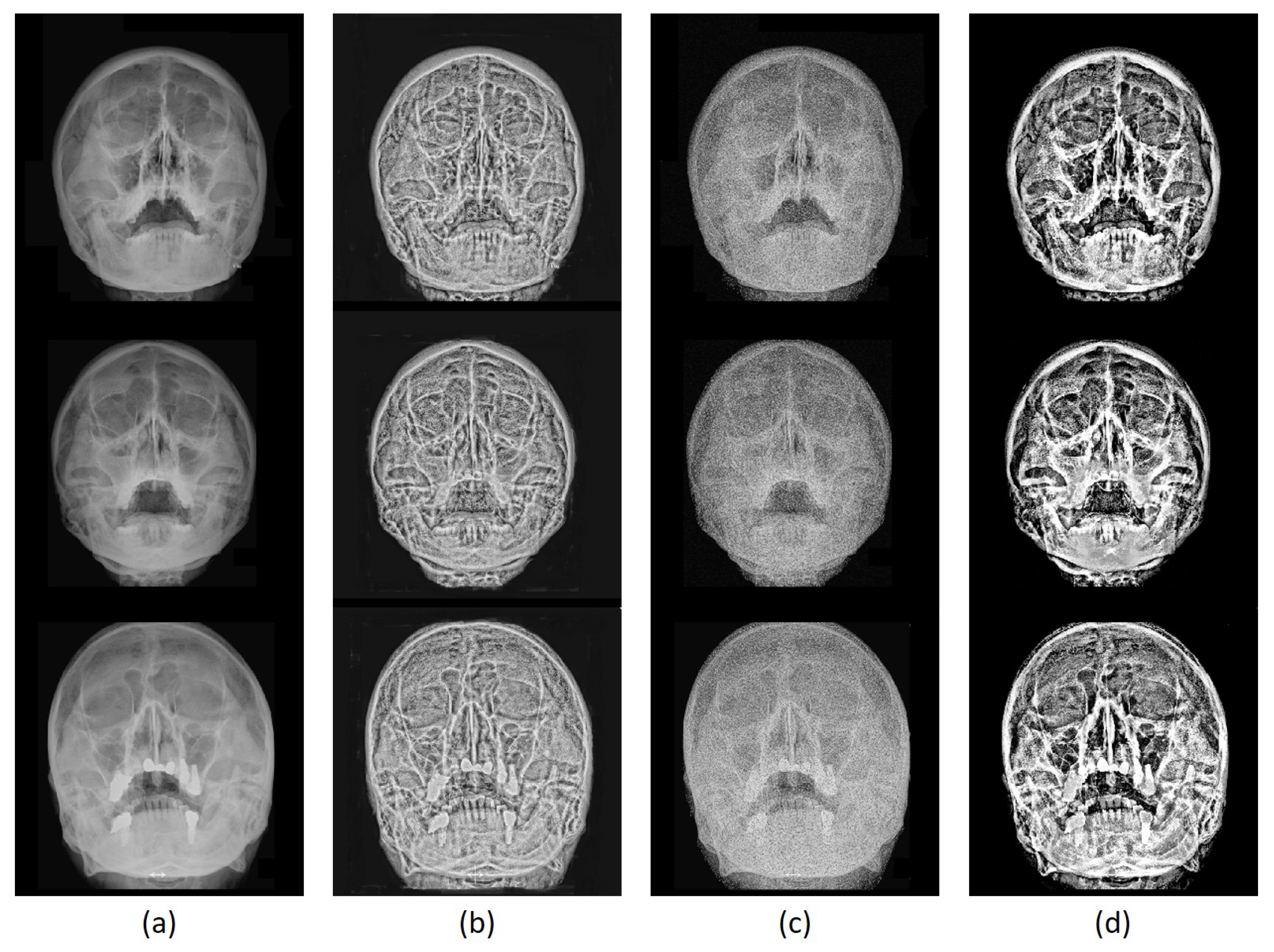
3.3. Image Enhancement Evaluation

3.3.1. Quantitative Evaluation

For assessments, various contrast evaluation metrics are implemented. Firstly, the Contrast Difference ($CD$) defines the contrast differences between input I and enhanced O images, where bright and dark features are similar in Reference [22] to:

$$CD=|C_I-C_O|,$$

(14)

where $C_I$ and $C_O$ denote Michelson contrast comparison of input and output, respectively. Therefore, the image contrast is measured as:

$$C_I=\frac{\underset{t\in T}{\max }I\left(t\right)-\underset{t\in T}{\min }I\left(t\right)}{\underset{t\in T}{\max }I\left(t\right)+\underset{t\in T}{\min }I\left(t\right)},$$

(15)

where t is any pixel located in the region of interest, namely T. $C_O$ is also calculated like Equation (15). High $CD$ represent improvement of contrast on images.

3.3.2. Qualitative Evaluation

Secondly, the Combined Enhancement Measure ($CE$) calculates the ratio of contrast between I and O over T against Z [23]. This metric is constructed based on three aspects:

$$CE=\sqrt{{(1-DS)}^2+{(1-TB{C}_{\sigma })}^2+{(1-TB{C}_{ϵ})}^2}.$$

(16)

The $DS$ in Equation (16) represents the overlapping pixel distribution area T and Z, while $TB{C}_{\sigma }$ and $TB{C}_{ϵ}$ measures the improvement of intensity and homogeneity ratios, respectively, between T and Z before and after enhancement. Smaller $CE$ corresponds to better enhancement method. Finally, the Contrast Improvement Index (CII) is used to calculate the contrast ratio before and after enhancement [24] as:

$$CII=\frac{({\mu }_T^I-{\mu }_Z^I)\times ({\mu }_T^I+{\mu }_Z^I)}{({\mu }_T^O+{\mu }_Z^O)\times ({\mu }_T^O-{\mu }_Z^O)}.$$

(17)

High $CII$ indicates a quality improvement of I on O.

To benchmark the performance of the proposed method, two prior state-of-the-arts in the contrast enhancement methods [7,8] were tested on the $OSXR$ dataset. Based on $CD$ scores in

Table 3. Comparisons of the prior and proposed contrast enhancements. ToMA = texture-based morphological analysis; CD = Contrast Difference; CE = Contrast Enhancement; CII = Contrast Improvement Index.

Metric	HM-CLAHE [7]			LCE-BSESCS [8]			Proposed ToMA
	N	P	U	N	P	U	N	P	U
$CD$	0.39	0.40	0.39	0.48	0.49	0.47	0.65	0.66	0.63
$CE$	1.73	1.73	1.73	0.83	0.77	0.80	0.17	0.12	0.12
$CII$	2.78	1.64	1.07	0.85	0.84	0.85	54.32	36.18	28.31

, both prior methods are lower in $CD$ scores compared with the proposed technique. These findings may confer that both prior methods [7,8] are still able to improve the image contrast but with lower improvement index than the ToMA offers.

In addition, Table 3 shows the average index of $CE$ for both prior methods with around 14.5 and 7 folds higher than the $CE$ index of ToMA, respectively. Based on this finding, the proposed method suggests better image enhancement. Furthermore, the inferior $CE$ indexes suggest that ToMA was able to remove overlapping pixel distribution between T and Z with high $DS$ index by preserving details in $TB{C}_{\sigma }$ and $TB{C}_{ϵ}$.

Furthermore, based on the $CII$ scores in Table 3, the proposed method outperforms the prior arts at an average of 39.60. Even though the $CII$ value of ToMA for all folds are wider than the prior methods, compared to prior methods, ToMA is still better in improving contrasts.

The qualitative observation shows the usability of enhanced SXRs in the actual medical diagnostic. A group of otolaryngologists were hired independently to perform diagnoses of sinusitis over enhanced SXRs. The results were than compared with the reference diagnosis data. Based on

Table 4. Performance of the proposed method from medical perspective.

Fold Type	Diagnosis	Data Amount	True Negative/True Positive
U	True Negative	64	0.84
	False Positive	12
	True Positive	11
	False Negative	2

, the enhanced SXRs from the unknown fold were able to increase the diagnosis accuracy of medical experts from 0% to 84%. This condition may suggest the effectiveness of the proposed ToMA in improving the diagnosis quality to possibly exclude CT screening from the procedure.

Figure 3 illustrates a montage of SXR resultants from the implemented techniques. The enhanced SZRS from HM-CLAHE in Figure 3b suggested a noticeable improvement, where the bone to soft-tissues are displayed clearly. Yet, there is much information on the enhanced SXR that were not enhanced properly, making it ambiguous to perform diagnosis. On the other hand, the LCE-BSESCS technique was able to keep details with distinct boundaries between bones and other soft-tissues; yet the contrast was not improved (Figure 3c). This condition may be the reason for the low $CII$ scores in LCE-BSESCS in Table 3.

Contrary to the previous methods, ToMA achieved substantial enhancement on SXRs particularly on boundaries of bone and soft-tissues as shown in Figure 3d. The air spaces on the dark features are conditioned to be highly dark while the pixel values of mucous fluids are made higher. This condition helps the diagnosis to be more straightforward yet accurate, such as in Figure 3d. Ambiguous textures within the region of interest as shown in Figure 3d are also reduced by increasing the dark features (i.e., the air-filled regions). Compared to the prior arts, the proposed ToMA is able to modify the distinctive features between the air- to fluid-containing regions of the maxillary sinuses.

3.3.3. Complexity Evaluation

According to

Table 5. Time cost of prior and proposed contrast enhancements.

Method	Time Cost (seconds)
	Negative Fold	Positive Fold	Unknown Fold
HM-CLAHE [7]	154.14	152.06	151.55
LCE-BSESCS [8]	107.74	93.63	102.46
Proposed Method	26.46	26.19	26.35

, the proposed ToMA has a lofty complexity due to rotational texture analysis that uses serial programming technique instead of the parallel programming. Yet, ToMA achieved 4 times and 6 times quicker than LCE-BSESCS and HM-CLAHE, respectively. Consequently, the complexity of the proposed ToMA can be reduced through code optimization or implementation of parallel programming.

3.4. Image Segmentation Evaluation

Quantitative Evaluation

The prior and proposed image segmentation were trained and tested using SXRs in $OSXR$ or $ESXR$ dataset. Each result ($O_d$) was assessed based on the corresponding ground truth ($G_d$) using various metrics. Firstly, the Jaccard similarity index (${\mathsf{\Omega }}_{JS}$) measures the similarity of finite sets (positive and negative pixels) in $O_d$ against the sets in $G_d$ map as:

$${\mathsf{\Omega }}_{JS}=\frac{|O_d\wedge G_d|}{|O_d\vee G_d|}=\frac{\left|TP\right|}{\left|FP\right|+\left|TP\right|+\left|FN\right|},$$

(18)

where $TP$ shows the number of correct pixels from output. $FP$ and $FN$ represent the falsely classified pixels as either ROI or background class, respectively. Secondly, the Dice similarity index (${\mathsf{\Omega }}_{QS}$) is a semimetric version of ${\mathsf{\Omega }}_{JS}$ that is more sensitive to observing overlapping pixels between $O_d$ and $G_d$ maps, expressed as:

$${\mathsf{\Omega }}_{QS}=\frac{|O_d\wedge G_d|}{|O_d|+|G_d|}=\frac{2\left|TP\right|}{\left|FP\right|+2\left|TP\right|+\left|FN\right|}.$$

(19)

Finally, the average contour distance ($\overline{X_c}$) computes the contour distance by taking the statistical average of the nearest contour distances between $O_d$ and $G_d$ maps. Suppose that $B_{O_d}\left(p\right)$ and $B_{G_d}\left(q\right)$ denote the boundary points within the maxillary sinuses on the $O_d$ and $G_d$ maps, respectively; The nearest distances from $O_d$ to $G_d$ and from $G_d$ to $O_d$ can be calculated as:

$$X_C^{O_d\to G_d}=\underset{q}{\min }\left|\right|B_{G_d}\left(q\right)-B_{O_d}\left(p\right)\left|\right|,$$

(20)

and

$$X_C^{G_d\to O_d}=\underset{p}{\min }\left|\right|B_{O_d}\left(p\right)-B_{G_d}\left(q\right)\left|\right|.$$

(21)

Subsequently, these average distances from Equations (20) and (21) are composed altogether to find the average contour distance as:

$${\overline{X}}_c=\frac{1}{2}(\frac{{\sum }_p\left[X_C^{O_d\to G_d}\right]}{n\left(B_{O_d}\right)}+\frac{{\sum }_q\left[X_C^{G_d\to O_d}\right]}{n\left(B_{G_d}\right)}).$$

(22)

By computing the ${\overline{X}}_c$ metric, the semantic data within the resulting segmentation results can be evaluated quantitatively.

The subjects of experiments for the evaluations of D-CNN image segmentation are limited between the proposed T-FCN and the prior FCN [16]. All possible combinations of method and dataset were evaluated and compared in order to understand a particular combination with the most optimum performance in both segmentation accuracy and architecture complexity. Since the network architecture in T-FCN requires multiple learning processes while the number of data in either ${\mathbf{S}}_{train}$ or ${\mathbf{S}}_{train}^o$ is limited, the T-FCN was only trained with two rounds of learning rounds. At $lr=0$, the T-FCN network had been trained using the Sunnybrook Left Ventricle Segmentation Challenge Dataset [25] to generate the 0-th pretrained model. Although Reference [25] yields an MRI of human left ventricle, it holds an uncanny relationship with both $OSXR$ and $EXSR$ because of the similarity in its functionality. Later, the weights from 0-th pretrained model were reconfigured on the $lr=1$, where the T-FCN network was being trained using either $OSXR$ or $ESXR$ dataset.

In

Table 6. Performance comparisons between the prior and proposed D-CNN-based methods on different test datasets.

Metric	FCN [16]		T-FCN
	$\mathit{OSXR}$	$\mathit{ESXR}$	$\mathit{OSXR}$	$\mathit{ESXR}$
${\mathsf{\Omega }}_{JS}$	0.628	0.699	0.717	0.756
${\mathsf{\Omega }}_{QS}$	0.755	0.819	0.829	0.857
${\overline{X}}_c$	306.8	95.03	132.5	33.69

, comprehensive comparisons on the performance of the T-FCN and FCN are presented using the aforementioned metrics. According to Table 6, the T-FCN model that had been trained on either $OSXR$ or $ESXR$ dataset achieved better average scores on all metrics compared to FCN model that had been trained on either $OSXR$ or $ESXR$ dataset. The segmentation accuracy of T-FCN using $ESXR$ dataset reached 85.7%, as verified with ${\mathsf{\Omega }}_{QS}$ metric that is over than the prior state-of-the-art, which achieved an accuracy of 81.9%. Comparatively, the T-FCN (in more details) achieved an average increase of ${\mathsf{\Omega }}_{JS}$ at 9.912% and ${\mathsf{\Omega }}_{QS}$ at 6.643%, where the average $\overline{X_c}$ is 1.5 times smaller than the FCN on both datasets. Consequently, the T-FCN for segmentation of maxillary sinuses on SXRs (either original or enhanced) provides higher accuracy compared to FCN.

From the information in Table 6, the effectiveness of the proposed ToMA algorithm for contrast enhancement is also inferred. According to the averages of ${\mathsf{\Omega }}_{JS}$ and ${\mathsf{\Omega }}_{QS}$ in Table 6, both FCN and T-FCN achieved significantly higher scores when trained on the $ESXR$ dataset compared to the $OSXR$ dataset. Significant effect on the utilization of $ESXR$ datasets can be seen on the $\overline{X_c}$ values of either FCN or T-FCN using $ESXR$ that are roughly 3.2 or 3.9 times smaller, respectively, than the $\overline{X_c}$ values of either FCN or T-FCN using $OSXR$. Based on this condition, the T-FCN model using $ESXR$ datasets provides the most optimum quality of image segmentation for maxillary sinuses.

4. Discussion

In both FCN [16] and T-FCN, with either $OSXR$ or $ESXR$ dataset, steep ${\mathsf{\Omega }}_{QS}$ scores for negative SXRs were achieved. As shown in Figure 4a–d, all combinations successfully segmented both left and right maxillary sinuses due to the features within the cavity walls can be easily identified as there is no discrepancy that attenuates those features.

Contrary to the prior example of negative cases, the positive cases of maxillary sinusitis induce complex textures within the inflamed sinus(es). In Figure 4e–h, the subject suffered acute sinus infection that causes substantial mucous accumulation within the left maxillary sinus, while the right maxillary sinus remained normal. This specific condition has made the cavity walls within the left maxillary sinus are vaguely depicted. Trained on $OSXR$ dataset, both methods adversely failed to segment the left maxillary sinus on the original SXR image shown in Figure 4e,g, respectively; yet, the right maxillary sinus was correctly segmented with better contour resemblance by T-FCN.

On the other hand, both FCN and T-FCN that were trained on $ESXR$ dataset generated better segmentation results, where both left and right maxillary sinuses were correctly segmented as shown in Figure 4f,h, respectively. Therefore, based on the comparison between methods trained with $OSXR$ and methods trained with $ESXR$, the observation suggested that the ToMA algorithm applied on SXRs from the $OSXR$ dataset to generate the $ESXR$ dataset is indeed effective in enhancing the performance of segmentation methods as the features are visually bolstered. Compared to FCN, the proposed T-FCN still showed its merit as FCN yields higher amount of false positive pixels on the left maxillary sinus because of strong boundary features from the lower zygomatic bone, which made false contours. Essentially, the FCN [16] is less robust against false contour(s) that may directly affect the actual contour of the maxillary sinuses compared to the proposed T-FCN.

For cases with dubious diagnosis in the unknown folds (including unknown-negative $U-N$ and unknown-positive $U-P$ cases), the proposed T-FCN with $ESXR$ dataset is consistent to be the most optimum combination to segment maxillary sinuses from the SXR images. In particular, the example in Figure 4i–l, shows that the proposed T-FCN trained with either $OSXR$ or $ESXR$ outperformed the prior FCN [16] trained with the corresponding dataset. The prior FCN with $OSXR$ dataset generated a significant amount of false predictions (shown in Figure 4i) because of low contrast condition after the image acquisition. On the other hand, the proposed T-FCN with $ESXR$ dataset generated segmentation result with most resemblance to the contour reference on both left and right sinuses (Figure 4l). The proposed ToMA that enhances the contrast ratio of the SXR images helped the T-FCN to extract and process the regions’ features correctly for accurate prediction outcomes.

Contrary to the prior example, instances in Figure 4m–p illustrate the unknown-positive with (a) dubious regions’ contours (because of infection) and (b) particularly unusual pose of the subject patient that obstructed the visibility of the left maxillary sinus. Subjectively, the prior FCN with $OSXR$ dataset failed to segment the left maxillary sinus (Figure 4m), while the other combinations of methods and datasets generated segmentation with better predictions (Figure 4n–p). For either right or left maxillary sinus, the proposed T-FCN with $ESXR$ provides the best segmentation among the others.

4.1. Complexity Evaluation

According to

Table 7. Time cost of prior and proposed image segmentation.

Consumption	FCN [16]		T-FCN
	$\mathit{OSXR}$	$\mathit{ESXR}$	$\mathit{OSXR}$	$\mathit{ESXR}$
Learning	541	283	7 ($lr=0$)	7 ($lr=0$)
(mins)			522 ($lr=1$)	284 ($lr=1$)
Inference	1.67	1.58	1.56	1.53
(secs/image)

, the FCN [16] with $ESXR$ dataset achieved the lowest time consumed for learning process with 283 min. Comparatively, the proposed T-FCN with $ESXR$ dataset achieved marginally higher time consumed for the learning process, with a total of 291 min (i.e., 284 + 7 min). This condition was advised as the T-FCN comprises of two learning processes. Nevertheless, the time difference between the prior and the proposed method with $ESXR$ dataset is as low as 8 min, which is negligible. Interestingly, the time consumed for the learning process by either method using $ESXR$ dataset is roughly 50% faster than the time consumed for the learning process by either method using the $OSXR$ dataset. This finding shows that the $ESXR$ dataset helps the learning process of both the T-FCN or the FCN [16] by shortening the effort to achieve convergence.

Based on the trained model from the corresponding combination of methods and datasets, the average times to process each SXR image in ${\mathbf{S}}_{test}^o$ of the $OSXR$ dataset or ${\mathbf{S}}_{test}$ of the $ESXR$ dataset are also listed in Table 7. According to Table 7, the average time to segment maxillary sinuses of an SXR image of all models is similar; yet the proposed T-FCN with $ESXR$ dataset achieved the lowest time cost to segment the SXR image at 1.53 s/image.

4.2. Study Limitation

The proposed methodology is implemented only on the visual enhancement of air-fluid contents in the maxillary sinus and occipitomental-view SXR images; thus, it shall only be able to segment maxillary sinuses. Although the proposed framework may be implemented on other image modalities, such as segmenting nodules on chest radiographs or masses on mammographs, this study only focused on the segmentation of maxillary sinuses for SXR images.

5. Conclusions

This study presented a CAD system that hand-in-hand improves the contrast of SXRs and performs segmentation over maxillary sinus regions. The proposed contrast enhancement is able to improve the contrast of SXR images with lowest complexity among the prior arts, while also increasing the diagnosis quality of SXR images with accuracy at 83.5%, true negative rate at 86.2%, and true positive rate of 78.9%. The proposed T-FCN enables periodic and continuous learning of the network that increases the model’s accuracy as more learning rounds were performed. When paired with the enhanced SXR images, the proposed T-FCN achieves segmentation accuracy of 85.70% with reduced learning time of up to 50% compared to the prior arts.

References

1. Hamilos, D.L. Chronic sinusitis. J. Allergy Clin. Immunol. 2000, 106, 213–227. [Google Scholar] [CrossRef] [Green Version]
2. Drumond, J.P.N.; Allegro, B.B.; Novo, N.F.; de Miranda, S.L.; Sendyk, W.R. Evaluation of the prevalence of maxillary sinuses abnormalities through spiral computed tomography (CT). Int. Arch. Otorhinol. 2017, 21, 126–133. [Google Scholar] [CrossRef] [PubMed] [Green Version]
3. Lazar, R.H.; Younis, R.T.; Parvey, L.S. Comparison of plain radiographic coronal CT and intraoperative findings in children with chronic sinusitis. Otolarnygol.-Head Neck Surg. 1992, 107, 29–34. [Google Scholar] [CrossRef] [PubMed]
4. Konen, E.; Faibel, M.; Kleinbaum, Y.; Wolf, M.; Lusky, A.; Hoffman, C.; Eyal, A.; Tadmor, R. The value of the occipitomental (Waters’) view in diagnosis of sinusitis: A comparative study with computed tomography. Clin. Radiol. 2000, 55, 856–860. [Google Scholar] [CrossRef] [PubMed]
5. Mettler, F.A.; Huda, W.; Yoshizumi, T.T.; Mahesh, M. Effective doses in radiology and diagnostic nuclear medicine: A catalog. Radiology 2008, 248, 254–259. [Google Scholar] [CrossRef]
6. Hussein, A.O.; Ahmed, B.H.; Omer, M.A.A.; Manafal, M.F.M.; Elhaj, A.B. Assessment of clinical x-ray and CT in diagnosis of paranasal sinus diseases. Int. J. Sci. Res. 2014, 3, 7–11. [Google Scholar]
7. Sundaram, M.; Ramar, K.; Arumugam, N.; Prabin, G. Histogram based contrast enhancement for mammogram images. In Proceedings of the International Conference of Signal Processing, Communication and Computer Network Technology, Thuckafay, India, 21–22 July 2011; pp. 842–846. [Google Scholar]
8. Ibrahim, H.; Hoo, S.C. Local contrast enhancement utilizing bidirectional switching equalization of separated and clipped subhistograms. Math. Probl. Eng. 2014. [Google Scholar] [CrossRef] [Green Version]
9. Zhou, Y.; Shi, C.; Lai, B.; Jimenez, G. Contrast enhancement of medical images using a new version of the World Cup Optimization algorithm. Quant. Imag. Med. Surgery 2019, 9, 1528–1547. [Google Scholar] [CrossRef]
10. Rundo, L.; Tangherloni, A.; Nobile, M.S.; Militello, C.; Besozzi, D.; Mauri, G.; Cazzaniga, P. MedGA: A novel evolutionary method for image enhancement in medical imaging systems. Expert Syst. Appl. 2019, 119, 387–399. [Google Scholar] [CrossRef]
11. Muslim, H.S.; Khan, S.A.; Hussain, S.; Jamal, A.A.; Qasim, H.S. A knowledge-based image enhancement and denoising approach. Comput. Math. Organ. Theory 2019, 25, 108–121. [Google Scholar] [CrossRef]
12. Nguyen, N.Q.; Lee, S.Q. Robust boundary segmentation in medical images using a consecutive deep encoder-decoder network. IEEE Access 2019, 7, 33795–33808. [Google Scholar] [CrossRef]
13. Garcia-Garcia, A.; Orts-Escolano, S.; Oprea, S.O.; Villena-Martinez, V.; Garcia-Rodriguez, J. A review on deep learning techniques applied to semantic segmentation. arXiv 2017, arXiv:1704.06857. [Google Scholar]
14. Weng, Y.; Zhou, T.; Li, Y.; Qiu, X. NAS-Unet: Neural architecture search for medical image segmentation. IEEE Access 2019, 7, 44247–44257. [Google Scholar] [CrossRef]
15. Zhang, G.; Dong, S.; Xu, H.; Zhang, H.; Wu, Y.; Zhang, Y.; Xi, X.; Yin, Y. Correction learning for medical image segmentation. IEEE Access 2019, 7, 143597–143607. [Google Scholar] [CrossRef]
16. Long, J.; Shelhamer, E.; Darrell, T. Fully convolutional networks for semantic segmentation. CoRR 2014, 2014, 1–10. [Google Scholar]
17. Zhao, W.; Zhang, h.; Yan, Y.; Fu, Y.; Wang, H. A Semantic Segmentation Algorithm Using FCN with Combination of BSLIC. Appl. Sci. 2018, 8, 500. [Google Scholar] [CrossRef] [Green Version]
18. Yasrab, R. ECRU: An Encoder-Decoder Based Convolution Neural Network (CNN) for Road-Scene Understanding. J. Imaging 2018, 4, 116. [Google Scholar] [CrossRef] [Green Version]
19. Jia, Y.; Shelhamer, E.; Donahue, J.; Karayev, S.; Long, J.; Girshick, R.; Guadarrama, S.; Darrell, T. Caffe: Convolution architecture for fast feature embedding. CoRR 2014, 2014, 675–678. [Google Scholar]
20. Alp’s Image Segmentation Tool. 2017. Available online: shorturl.at/fjopM (accessed on 30 September 2017).
21. Wei, Q.; Dunbrack, R.L. The role of balanced training and testing datasets for binary classifiers in bioinformatics. PLoS ONE 2013, 8, e67863. [Google Scholar]
22. Lado, M.J.; Tahoces, P.G.; Mendez, A.J.; Souto, M.; Vidal, J.J. A wavelet-based algorithm for detection clustered microcalcifications in digital mammograms. Med. Phys. 1999, 26, 1294–1305. [Google Scholar] [CrossRef]
23. Singh, S.; Bovis, K. An evaluation of contrast enhancement techniques for mammographic breast masses. IEEE Trans. Inf. Technol. Biomed. 2005, 9, 109–119. [Google Scholar] [CrossRef] [PubMed]
24. Morrow, W.M.; Paranjape, R.B.; Rangayyan, R.M.; Desautels, J.E.L. Region-based contrast enhancement of mammograms. IEEE Trans. Med. Imaging 1992, 11, 392–406. [Google Scholar] [CrossRef] [PubMed]
25. Radau, P.; Lu, Y.; Connelly, K.; Paul, G.; Dick, A.J.; Wright, G.A. Evaluation framework for algorithms segmenting short axis cardiac MRI. MIDAS J. 2009, 49. Available online: http://hdlhandlenet/10380/3070 (accessed on 9 May 2020).
Figure 1. A step-by-step diagram of the image contrast enhancement for skull X-rays (SXRs) using proposed texture-oriented morphological analysis.
Mathematics 08 00768 g001
Figure 2. Illustration of occipitomental-view skull radiography (SXR) dataset. The negative (N) and the positive (P) folds are containing plain SXR images. The unknown-negative (U-N) and the unknown-positive (U-P) folds are containing plain SXR images with dubious features.
Mathematics 08 00768 g002
Figure 3. Experimental result montages of various enhancement schemes. (a) Original SXR images from the negative N, the positive P, and the unknown folds ( U N , U P ) of the dataset (top–bottom). (b) Enhanced images from the HM-CLAHE [7]. (c) Enhanced images from the LCE-BSECSC [8]. (d) Enhanced images from the proposed ToMA method.
Mathematics 08 00768 g003
Figure 4. A montage of segmentation results using the FCN [16] against the T-FCN with all combinations of training and test datasets as shown above from (ap).
Mathematics 08 00768 g004