Computational Bifurcations Occurring on Red Fixed Components in the λ-Parameter Plane for a Family of Optimal Fourth-Order Multiple-Root Finders under the Möbius Conjugacy Map

Abstract

Optimal fourth-order multiple-root finders with parameter $\lambda$ were conjugated via the Möbius map applied to a simple polynomial function. The long-term dynamics of these conjugated maps in the $\lambda$-parameter plane was analyzed to discover some properties of periodic, bounded and chaotic orbits. The $\lambda$-parameters for periodic orbits in the parameter plane are painted in different colors depending on their periods, and the bounded or chaotic ones are colored black to illustrate $\lambda$-dependent connected components. When a red fixed component in the parameter plane branches into a q-periodic component, we encounter geometric bifurcation phenomena whose characteristics determine the desired boundary equation and bifurcation point. Computational results along with illustrated components support the bifurcation phenomena underlying this paper.

1. Introduction

The governing equations of natural phenomena are usually represented as nonlinear equations in the form of $f\left(x\right)=0$, when solving the relevant algebraic or differential equations obtained through the scientific observations, experiments, experiences as well as mathematical modeling. Since the exact solutions of such nonlinear governing equations are rarely feasible, it is considered best to rely on numerical solution techniques such as multi-point iterative methods [1,2,3,4], splitting methods [5,6], semi-explicit methods [7,8] as well as analytical-numerical methods [9]. Among such techniques, the most widely used multi-point iterative method under general circumstances is Newton’s method which converges quadratically to a simple root and linearly to a multiple root. In order to more accurately solve the nonlinear governing equations, many researchers have been developing new iteration methods with high convergence orders, including Newton’s method as a particular case. Motivation for writing this paper is to analyze the convergence behavior of these iterative numerical methods from the viewpoint of the limit behavior under the iteration dynamics with illustrative computational results.

Although the limit behavior of the aforementioned numerical solution techniques draws great attention to the readers, our study will focus on the limit behavior of a family of Newton-like iterative methods with a simple structure of a weight function possessing a $\lambda$-control parameter. The convergence behavior of these iterative numerical methods equipped with $\lambda$-control parameters can be analyzed from a viewpoint of iteration dynamics. Let us begin with a family of nonlinear governing equations with parameter $\lambda$ as represented by the following nonlinear recurrence relation:

$$x_{n+1}=W_f(\lambda ;x_n),n=0,1,2,\cdots ,$$

(1)

where $W_f$ is called the iteration function or fixed point operator [10]. If iteration index n is regarded as an indicator of time, then the nonlinear recurrence relation (1) would represent itself the relevant discrete dynamical system. Consequently, pursuing the convergence of the root of the nonlinear recurrence relation (1) is initiated by dealing with its limit behavior under the action of the nonlinear discrete dynamical system (1). The governing equation to be dealt with in this paper is a family of optimal [11] two-point Newton-like fourth-order multiple–root finders with parameter $\lambda$ studied in Reference [3]:

$$\left\{\begin{array}{c}{y}_n=x_n-m·\frac{f\left(x_n\right)}{f^{\prime }\left(x_n\right)},\hfill \\ x_{n+1}=x_n-m·Q_f(\lambda ;t)·\frac{f\left(x_n\right)}{f^{\prime }\left(x_n\right)}=W_f(\lambda ;x_n),t={\left[\frac{f\left(y_n\right)}{f\left(x_n\right)}\right]}^{1/m},\hfill \end{array}\right.$$

(2)

where $Q_f:{\mathbb{C}}^2\to \mathbb{C}$ is analytic [12] in a neighborhood of $(\lambda ,0)$ with $\lambda \in \mathbb{C}$ fixed and t is taken on the principal analytic branch of the m-th root. In the current study, we will employ a specific form of $Q_f$ with a controllable parameter $\lambda \in \mathbb{C}$ as follows:

$$\begin{array}{c}{Q}_f(\lambda ;t)=\frac{1+(\lambda +1)t+(\lambda +2)t^2}{1+\lambda t}.\hfill \end{array}$$

(3)

The advantage of choosing such a rational function $Q_f$ is to allow the conjugated $W_f$ to contain the low-order polynomial factor $T(\lambda ;z)$ with exact $\lambda$-dependent roots, that is, the exact fixed points of $\mathcal{F}$ from fixed-point relation (6) under the Möbius conjugacy to be introduced in Section 4. If a different type of $Q_f$, say, a polynomial were chosen, then the higher order of $T(\lambda ;z)$ would hinder us from locating the exact fixed points.

In Reference [13], as a part of long-term dynamics for the conjugated map of (2), a study was conducted on bifurcation [14,15] phenomena occurring on the boundary curve of the yellow fixed component related to $\lambda$-free strange fixed point $z=1$. The number of the component was turned out to be only one. Moreover, the equation of the boundary curve turned out to be a circle as one of the known geometric shapes. This simple circle allowed us to analyze the global bifurcations occurring on it without difficulties.

The aim of this paper is to study of the fixed points under the Möbius conjugacy map and to investigate in depth the boundary curves and other geometric properties of the hyperbolic components [16] in the $\lambda$-parameter plane (to be defined in Section 4). The current study will cover a challenging task not handled in the previous study in Reference [13]. We will extensively investigate the bifurcation phenomena of the red fixed component ${\mathcal{R}}^f$ (whose notation and analysis will be described in Section 3 and Section 4) related to the strange fixed point $z=z\left(\lambda \right)$, which is $\lambda$-dependent, that is, not $\lambda$-free as in the case of the previous study for the yellow fixed component. In particular, it is our curiosity and concern to find out whether the number of ${\mathcal{R}}^f$ is more than one, and whether the equation of the boundary curve represents a known geometric figure. From the perspective of plane geometric curves, our main interest lies in the computational, theoretical and visual exploration of bifurcation phenomena occurring on the boundary curve of ${\mathcal{R}}^f$.

A theoretical formulation of the boundary equation of ${\mathcal{R}}^f$ developed here will serve as a basis for describing bifurcation phenomena occurring in another discrete dynamical system. For example, it is helpful to establish the boundary equations of hyperbolic components with small periods in the Mandelbrot set [17] for a better analysis of bifurcation phenomena occurring there.

The remainder of this paper further describes the important points for the analysis of bifurcation phenomena. Described in Section 2 are preliminary results on the long-term behavior of a dynamical system and local bifurcations. In Section 3, we describe various properties of the fixed and critical points under the Möbius conjugacy map. Section 4 investigates a long-term dynamical behavior and the symmetry of the parameter plane. The location of the bifurcation points is extensively explored based upon the existence of a common osculating point between the fixed component (maximal connected set) [12] and q-periodic component. Section 5 describes the boundary curves of the fixed components along with their geometric properties. Finally in Section 6, we summarize overall studies and state the possible future work on the long-term dynamics of period-2 components.

2. Preliminary Results

Although iteration function $W_f$ in (1) is in general meromorphic, it suffices to treat the dynamics of rational functions only, in view of Lemma of 2.1 of Reference [13]. Indeed, we apply $f\left(z\right)={\left((z-a)(z-b)\right)}^m$ to obtain the conjugation of rational $W_f$, namely, $\mathcal{F}=h\circ W_f\circ h^{-1}$ in the form of a rational function to be shown in (4) via the first-order rational Möbius conjugacy map $h\left(z\right)=\frac{z-b}{z-a}$, with $a\ne b$ [18].

The following definition of conjugacy and other assertions are useful for continuing discussion of the relevant dynamics.

Definition 1.

Let$\mathcal{F}:D\subset \overline{\mathbb{C}}\to D$and$\mathcal{K}:E\subset \overline{\mathbb{C}}\to E$represent two dynamical systems. The dynamical system$\mathcal{F}$is said to be conjugate to$\mathcal{K}$via h if there exists an isomorphism$h:E\to D$such that$\mathcal{F}\circ h=h\circ \mathcal{K}$. Such h is called a conjugacy [19].

According to Theorem of 2.1 in Reference [13], we find:

Theorem 1.

Let$\mathcal{F},\mathcal{K}\in {\mathit{C}}^1$and be conjugate to each other via the diffeomorphic conjugacy h. In addition, let ξ be a fixed point of$\mathcal{K}$. Then the following hold:

(a) 

The fixed point property remains invariant under a topological conjugacy h, that is,

$$\xi =\mathcal{K}\left(\xi \right)ifandonlyifh\left(\xi \right)=\mathcal{F}\left(h\right(\xi \left)\right).$$

(b) 

The Poincaré characteristic multiplier [15] of ξ by$\mathcal{K}$, denoted by$m(\mathcal{K},\xi )$, is invariant under a diffeomorphic conjugacy h, that is,

$$m(h\circ \mathcal{K}\circ h^{-1},h\left(\xi \right))={\mathcal{F}}^{\prime }\left(h\left(\xi \right)\right)={\mathcal{K}}^{\prime }\left(\xi \right)=m(\mathcal{K},\xi ).$$

Remark 1.

If$\mathcal{F}$and$\mathcal{K}$are conjugate to each other via the topological conjugacy h, then we find$\mathcal{F}=h\circ \mathcal{K}\circ h^{-1}$and${\mathcal{F}}^n=(h\circ \mathcal{K}\circ h^{-1})\circ (h\circ \mathcal{K}\circ h^{-1})\cdots \circ (h\circ \mathcal{K}\circ h^{-1})$ = $h\circ {\mathcal{K}}^n\circ h^{-1}$. If $\mathcal{F}$ and $\mathcal{K}$ are further invertible, then we also find ${\mathcal{F}}^{-1}=h\circ {\mathcal{K}}^{-1}\circ h^{-1}$ and ${\mathcal{F}}^{-n}=h\circ {\mathcal{K}}^{-n}\circ h^{-1}$. Hence, the topological conjugacy h gives an isomorphism between two orbits of $\mathcal{F}$ and $\mathcal{K}$.

Letting $\mathcal{K}=W_f(\lambda ;z_n)$ in (2) yields ${\mathcal{F}}^n=h\circ W_f^n\circ h^{-1}$ for all $n\in \mathbb{Z}$. Then the orbit behavior of $\mathcal{F}$ exhibits a behavior similar to that of the iterative function $W_f$. According to Theorem 1, the invariant properties of the fixed point and the Poincaré characteristic multiplier after the conjugacy transformation address that $\mathcal{F}$ and $W_f$ have the advantage that their orbit dynamics is invariant. Such an advantage may give the favorable geometric characteristics induced by the orbit behavior of $\mathcal{F}$.

Lemma 1.

Suppose that$\psi :\Omega \subset \overline{\mathbb{C}}\to \Omega$is meromorphic and has a fixed point$\xi \in \Omega$with$|{\psi }^{\prime }(\xi )|<1$. Then ψ has a unique fixed point ξ such that sequence${\{z_{n+1}=\psi \left(z_n\right)\}}_0^{\infty }$converges to ξ for any given$z_0\in \Omega$.

Proof. 

(i) For $\xi \in \Omega \subset \mathbb{C}$, the proof is done by Lemma 1 of Reference [20]. (ii) For $\psi (\infty )=\infty$, it is possible to make $|{\psi }^{\prime }(\infty )|<1$ under some restrictions on the form of $\psi$, which can be justified based on the following description. By definition from Section 3.1 of Reference [21], $\psi$ is said to be analytic at ∞ if $H\circ \psi \circ H^{-1}$ is analytic at 0 with $H\left(z\right)=1/z$. Due to Lemma 2.1 of Reference [13], we can express $\psi \left(z\right)=\frac{a_0+a_{1}z+\cdots +a_n{z}^n}{b_0+b_{1}z+\cdots +b_m{z}^m}$ as a rational function with $a_n{b}_m\ne 0,n>m$ for $n,m\in \mathbb{N}\cup \left\{0\right\}$. We further define a function $S\left(z\right)\equiv H\circ \psi \circ H^{-1}\left(z\right)=\frac{1}{\psi (1/z)}$ and find ${\psi }^{\prime }(\infty )=S^{\prime }\left(0\right)=\left\{\begin{array}{cc}{b}_m/a_n,\hfill & ifn=m+1\hfill \\ 0,\hfill & ifn>m+1\hfill \end{array}\right.$ by direct computation or from Section 2.6 of Reference [19]. Hence if restriction $|{\psi }^{\prime }(\infty )|=|\frac{b_m}{a_n}|<1$ is made, then ∞ becomes an attracting fixed point of $\psi$. □

If we select $z_0$ as a critical point $z^{*}$ of $\psi$ satisfying ${\psi }^{\prime }\left(z^{*}\right)=0$, then Lemma 1 with $z_0=z^{*}$ yields the following corollary.

Corollary 1.

Let$q\in \mathbb{N}$and ξ be an attracting q-periodic point of ψ in Lemma 1. Then every critical orbit of ψ tends to ξ.

Corollary 1 will theoretically support the formation of hyperbolic components serving as important parts of the structure of the parameter space to be introduced later in Section 4.

We now define a function $G(\lambda ;z)={\psi }_{\lambda }\left(z\right)$ for a given parameter $\lambda \in \mathbb{C}$. Let $\xi$ and $\omega$ respectively denote a fixed point and a critical point of $G(\lambda ;z)$. Then, in view of Lemma 1, $\left|\frac{d}{dz}G(\lambda ;\xi )\right|=\left|G^{\prime }(\lambda ;\xi )\right|=\left|{{\psi }_{\lambda }}^{\prime }\left(\xi \right)\right|=1$ would influence the long-term orbit behavior of $G(\lambda ;\omega )$ as the parameter $\lambda$ varies across the boundary of region $\Omega \subset \mathbb{C}$. The unit circle characterizes the stability $G^{\prime }(\lambda ;\xi )$ and is better designated as the stability unit circle S for further analysis.

An abrupt change of such a long-term orbit behavior of $G(\lambda ;\omega )$ often arises at $\lambda ={\lambda }^{*}$, where the value of $G^{\prime }(\lambda ;\xi )$ crosses the boundary of S. This kind of abrupt change in its dynamical behavior is said to be a bifurcation. Consulting the notions of such bifurcations in Reference [22], the following three types of bifurcation may occur:

(1)

If $G^{\prime }({\lambda }^{*};\xi )=1$, then the bifurcation is of (cyclic) fold(saddle-node).

(2)

If $G^{\prime }({\lambda }^{*};\xi )=-1$, then the bifurcation is of flip(period-doubling).

(3)

If $G^{\prime }({\lambda }^{*};\xi )=e^{i\theta }$, then the bifurcation is of Neimark-Sacker(secondary Hopf),

with $\theta \ne \pi ,0<\theta <2\pi$.

Such a control parameter ${\lambda }^{*}$ in the parameter plane is called a bifurcation point whose location will be treated in Section 4.2.

3. Fixed and Critical Points under a Linear Fractional Möbius Conjugacy Map

The conjugated map of (2) under a linear fractional Möbius conjugacy map applied to a polynomial $f\left(z\right)={\left((z-a)(z-b)\right)}^m$ will be investigated regarding the relevant properties underlying its fixed and critical points for $\lambda \in \mathbb{C}$. We will explore its long-term dynamical behavior [10,18,23,24,25,26,27] behind the parameter plane via a linear fractional conjugacy map which is given by the Möbius conjugacy map $h\left(z\right)=\frac{z-b}{z-a}$, with $a\ne b$. Let $\mathcal{F}=h\circ W_f\circ h^{-1}$. Then the resulting $\mathcal{F}$ represents:

$$\mathcal{F}(\lambda ;z)=\frac{z^4(5+4z+z^2+\lambda (z+2))}{q(\lambda ;z)}=\frac{z^6(q(\lambda ;\frac{1}{z})}{q(\lambda ;z)},$$

(4)

where $q(\lambda ;z)=1+z(4+\lambda )+z^2(5+2\lambda )$. Be aware that conjugacy $h\left(z\right)$ makes $\mathcal{F}(\lambda ;z)$ free from parameters $m,a,b$. In addition, we directly compute the derivative of $\mathcal{F}$ from (4):

$${\mathcal{F}}^{\prime }(\lambda ;z)=\frac{2z^3{(z+1)}^{2}Q(\lambda ;z)}{q{(\lambda ;z)}^2},$$

(5)

where $Q(\lambda ;z)=10+4\lambda +z(20+14\lambda +3{\lambda }^2)+2z^2(5+2\lambda )$.

The $\lambda$-dependent fixed points of $\mathcal{F}(\lambda ;z)$ are given by the roots of

$$\mathcal{F}(\lambda ;z)-z=\frac{z(z-1)·T(\lambda ;z)}{q(\lambda ;z)},$$

(6)

where $T(\lambda ;z)=1+z(5+\lambda )+z^2(10+3\lambda )+z^3(5+\lambda )+z^4$.

Consulting Sections 3.1 and 3.2 of Reference [20], we state following proposition for properties of $\mathcal{F}$ and ${\mathcal{F}}^{\prime }$:

Proposition 1.

(a) 

If$\xi \in \overline{\mathbb{C}}$is a fixed point of$\mathcal{F}$, then so is$1/\xi$.

(b) 

If$\omega \in \overline{\mathbb{C}}$is a critical point of$\mathcal{F}$, then so is$1/\omega$.

(c) 

Relation$\mathcal{F}(\lambda ;\frac{1}{z})=\frac{1}{\mathcal{F}(\lambda ;z)}$holds for any$\lambda \in \mathbb{C}$and any$z\in \overline{\mathbb{C}}$.

(d) 

Relation${\mathcal{F}}^{\prime }(\lambda ;\frac{1}{\xi })={\mathcal{F}}^{\prime }(\lambda ;\xi )$holds for any$\lambda \in \mathbb{C}$and any fixed point$\xi \in \overline{\mathbb{C}}$of$\mathcal{F}$.

According to Theorem 1-(a), the fixed points 0 and ∞ of $\mathcal{F}=h\circ \mathcal{K}\circ h^{-1}$ with $h\left(z\right)=\frac{z-b}{z-a},(a\ne b)$ and $\mathcal{K}=W_f$ respectively correspond to the fixed points a and b of $W_f$, that is, the roots of polynomial $f\left(z\right)={(z-a)}^m{(z-b)}^m$. They are super-attractive, free of $\lambda$ and also imply the critical points of $\mathcal{F}(\lambda ;z)$ in view of (5).

Nevertheless, because their orbits approach themselves, the dynamical impact is expected to be small. Fixed points excluding such fixed points $\{0,\infty \}$ are termed as strange fixed points [28] which are not the roots of $f\left(z\right)={(z-a)}^m{(z-b)}^m$. Notice that $z=1$ is a $\lambda$-free strange fixed point whose dynamics was explored in Reference [13]. The roots of $T(\lambda ;z)=0$ in (6) are indeed $\lambda$-dependent strange fixed points. Simple computations directly prove the following lemma.

Lemma 2.

$T(\lambda ;\frac{1}{z})=\frac{T(\lambda ;z)}{z^4}$and$Q(\lambda ;\frac{1}{z})=\frac{Q(\lambda ;z)}{z^2}$hold for any$\lambda \in \mathbb{C}$and any$z\in \overline{\mathbb{C}}$.

We seek $\lambda$-dependent strange fixed points ${\xi }_{\lambda }$ by solving $T(\lambda ;{\xi }_{\lambda })=0$ for a fixed $\lambda \in \mathbb{C}$. According to Proposition 1-(a), $T(\lambda ;z)$ can be written in the form: $T(\lambda ;z)={\prod }_{k=1}^2(z^2+c_{k}z+1)=0$, that is, $z=-\frac{1}{2}\left(c_k+\sqrt{c_k^2-4}\right)$ where $c_k,(1\le k\le 2)$ are the roots satisfying

$$c^2-c(\lambda +5)+3\lambda +8=0.$$

(7)

Hence, we are able to express all the desired $\lambda$-dependent strange fixed points of $\mathcal{F}$ as ${\xi }_{\lambda }^{\left(k\right)}$ and $1/{\xi }_{\lambda }^{\left(k\right)}$ with the notation ${\xi }_{\lambda }^{\left(k\right)}=-\frac{1}{2}\left(c_k+\sqrt{c_k^2-4}\right)$ for $1\le k\le 2$. Figure 4 of Reference [13] illustrates the stability surfaces of $\lambda$-dependent strange fixed points ${{\xi }_{\lambda }}^{\left(j\right)}(1\le j\le 2)$.

The super-attractors of $\mathcal{F}(\lambda ;z)$ can be found by solving $T(\lambda ;z)=Q(\lambda ;z)=0$ for z and $\lambda$. Eliminating z in $T(\lambda ;z)=Q(\lambda ;z)=0$ yields a 4-degree polynomial

$$(2+\lambda )(-100-50\lambda +8{\lambda }^2+3{\lambda }^3)=0,$$

(8)

from which we find $\lambda \in \{-4.7034,3.86866,-2,-1.83192\}$ for the desired super-attractors. Note that the cubic factor in (8) with positive discriminant value of $1,594,800$ has three distinct real roots.

On the other hand, eliminating $\lambda$ in $T(\lambda ;z)=Q(\lambda ;z)=0$ yields an 8-degree polynomial

$${(1+z)}^2(1+4z-4z^2-10z^3-4z^4+4z^5+z^6)=0,$$

(9)

which induces 8 supper-attractors denoted by 4 pairs of $(z_j,1/z_j)$ for $1\le j\le 4$ with $z_1=0.568254,z_2=-0.224773,z_3=-1$ and $z_4=-0.827167-0.561957i$. Lemma 2 leads us to only 4 pairs of super-attractors $(\lambda ;z)$ as follows:

$$(\lambda ;z)\in \left\{\right(-4.7034;0.568254),(3.86866;-0.224773),(-2;-1),(-1.83192;-0.827167-0.561957i\left)\right\}.$$

(10)

The critical points of $\mathcal{F}$ are given by the roots of ${\mathcal{F}}^{\prime }(\lambda ;z)=0$. A quick glance of (5) reveals that $z=-1$ is a $\lambda$-free critical point. Evidently $z=0$ and $z=\infty$ are critical points that respectively correspond to the roots a and b of the polynomial ${(z-a)}^m{(z-b)}^m$. The critical points excluding the both roots a and b are termed as free critical points [28]. Since the orbit behavior of $\lambda$-dependent critical point of $\mathcal{F}(\lambda ;z)$ draws our attention, we will treat free critical points that are $\lambda$-dependent.

4. Long-Term Orbit Behavior with Bifurcation Phenomena in the Parameter Plane

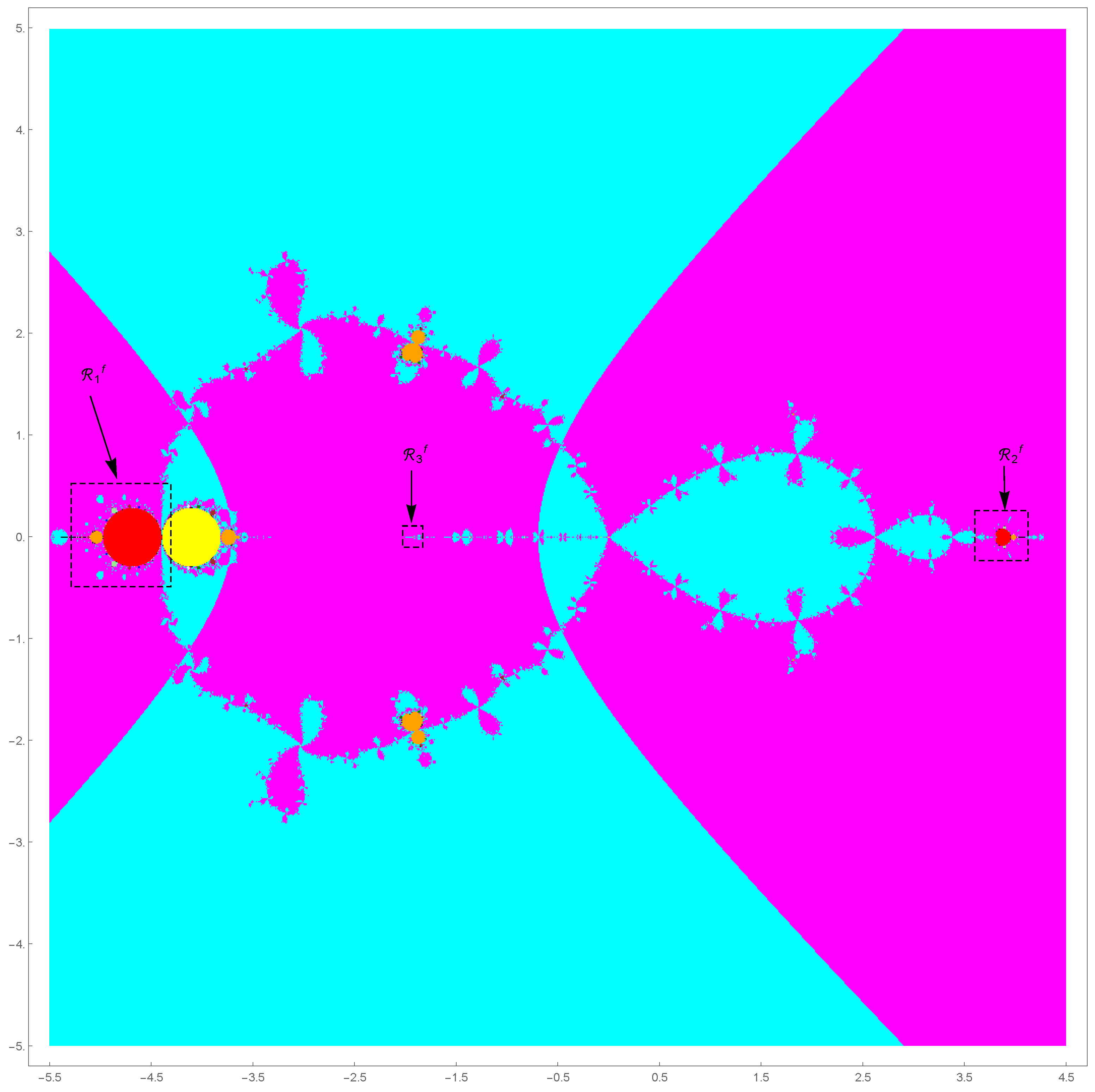
4.1. Parameter Plane and Long-Term Orbit Behavior

One way to efficiently handle the long-term orbit dynamics of the iterative map $\mathcal{F}(\lambda ;z)$ in (4) is to visually illustrate its dynamical orbit behavior in the $\lambda$-parameter plane whose definition will be made in this section. The long-term critical orbit under the action of $\mathcal{F}(\lambda ;z)$ will induce attracting periodic, finitely bounded or chaotic orbits for each given $\lambda$ selected in the $\lambda$-parameter plane. It is certainly interesting to paint the point $\lambda$ for which the long-term orbit approaches an attracting periodic orbit, with different color depending on its period.

Corollary 2 and Remark 2 well state the orbit behavior between two critical points z and $1/z$ of $\mathcal{F}$.

Corollary 2.

Let$q\in \mathbb{N}$be given. If$z\in \overline{\mathbb{C}}$is a q-periodic point of$\mathcal{F}(\lambda ;z)$, then so is$\frac{1}{z}$.

Proof. 

Lemma 2 directly shows that $\mathcal{F}(\lambda ;z)=z$ and $\mathcal{F}(\lambda ;1/z)=1/z$ for a fixed point z of $\mathcal{F}$ with a fixed $\lambda \in \mathbb{C}$. Hence there exists a topological conjugacy $h\left(z\right)=1/z$ such that $\mathcal{F}(\lambda ;z)=h\circ \mathcal{F}(\lambda ;z)\circ h^{-1}$ for a fixed point z. Hence, Remark 1 yields a relation ${\mathcal{F}}^q(\lambda ;z)=h\circ {\mathcal{F}}^q(\lambda ;z)\circ h^{-1}$. Clearly, ${\mathcal{F}}^q(\lambda ;z)=z$ gives ${\mathcal{F}}^q(\lambda ;\frac{1}{z})=\frac{1}{{\mathcal{F}}^q(\lambda ;z)}=\frac{1}{z}$, completing the proof. □

Remark 2.

Let${\omega }_1$and${\omega }_2$be the two λ-dependent critical points of$\mathcal{F}(\lambda ;z)$found from the roots of$Q(\lambda ;z)=0$in (5) shown below:

$${\omega }_1=\left\{\begin{array}{c}-\frac{20+14\lambda +3{\lambda }^2+\sqrt{3\lambda (2+\lambda )(4+\lambda )(10+3\lambda )}}{4(5+2\lambda )},if\lambda \ne \frac{5}{2}\hfill \\ \infty ,if\lambda =-\frac{5}{2}.\hfill \end{array}\right.and{\omega }_2=\frac{1}{{\omega }_1}.$$

(11)

If the orbit of${\omega }_1$approaches a q-periodic point${\xi }_1$of$\mathcal{F}$, then the orbit of${\omega }_2=\frac{1}{{\omega }_1}$also approaches a q-periodic point${\xi }_2=\frac{1}{{\xi }_1}$, by virtue of Corollary 2.

In light of Remark 2, it suffices to consider only one branch of the critical points ${\omega }_1$ for its typical orbit behavior. We define the parameter plane(space) $\mathcal{P}$ for iterative map $\mathcal{F}(\lambda ;z)$ as follows:

$$\begin{array}{c}\mathcal{P}=\{\lambda \in \mathbb{C}:\mathrm{an}\mathrm{orbit}\mathrm{of}\mathrm{a}\mathrm{critical}\mathrm{point}\omega \mathrm{tends}\mathrm{to}\mathrm{a}\mathrm{number}\gamma \in \overline{\mathbb{C}}\mathrm{under}\mathrm{the}\mathrm{action}\mathrm{of}\mathcal{F}(\lambda ;\omega )\}.\hfill \end{array}$$

From now on, let $\omega$ denote the critical point ${\omega }_1$ for convenience. Consider the limit behavior of an orbit of $\mathcal{F}(\lambda ;\omega )$ approaching a number $\gamma \in \overline{\mathbb{C}}$ in the long run. If $\gamma =\infty$, then it draws very little attention to the limit behavior since $\mathcal{F}(\lambda ;\infty )=\infty$. On the contrary, if $\gamma$ is finite, then it will create a diversity of the limit behavior as $\lambda \in \mathbb{C}$ varies. More importantly, if $\gamma$ is finite as well as bounded, then Bolzano-Weierstass Theorem guarantees the existence of a subsequence of the orbit of $\mathcal{F}(\lambda ;\omega )$ converging to the fixed point $\xi \left(\lambda \right)$. In other words, we can find a q-periodic point $\xi \left(\lambda \right)=\gamma$ for some $q\in \mathbb{N}$ in such a way that

$$\xi \left(\lambda \right)=\gamma =\underset{\ell \to \infty }{\lim }{\mathcal{F}}^{\ell }(\lambda ;\omega )=\underset{j\to \infty }{\lim }{\mathcal{F}}^{pj+q}(\lambda ;\omega )={\mathcal{F}}^q\circ (\underset{j\to \infty }{\lim }{\mathcal{F}}^{pj}(\lambda ;\omega ))={\mathcal{F}}^q(\lambda ;\xi \left(\lambda \right)),$$

(12)

by expressing $\ell =pj+q$ for any $\ell ,p,j\in \mathbb{N}$ with $p<\ell$ and $q\in \{0,1,2,\cdots ,p-1\}$; if $q=0$, then it suggests that a non-periodic bounded orbit could exist. As a result, the q-periodic orbit of $\xi \left(\lambda \right)=\gamma$ forms a q-cycle:

$$\left\{\xi \left(\lambda \right),\mathcal{F}(\lambda ;\xi \left(\lambda \right)),{\mathcal{F}}^2(\lambda ;\xi \left(\lambda \right)),\cdots ,{\mathcal{F}}^{q-1}(\lambda ;\xi \left(\lambda \right))\right\}.$$

(13)

Taking the discussion in Section 3 into consideration, we find the possible fixed points $\xi \left(\lambda \right)\in \{0,1,\infty ,{\xi }_{\lambda }^{\left(k\right)},1/{\xi }_{\lambda }^{\left(k\right)},(1\le k\le 2)\}$. We now define a function $G(\lambda ;z)={\mathcal{F}}^q(\lambda ;z)-z$ for any given $q\in \mathbb{N}$. As a consequence, $G(\lambda ;z)$ establishes a bivariate rational function of z and $\lambda$ on $\overline{\mathbb{C}}$. Since the rational function $G(\lambda ;z)$ has a finite number of zeros $z=\xi \left(\lambda \right)$, that is, the fixed points of ${\mathcal{F}}^q(\lambda ;z)$ for any given $q\in \mathbb{N}$, we can find a $\lambda$ for any periodic-point $z=\xi \left(\lambda \right)$ being approached by the long-term critical orbit of $\mathcal{F}(\lambda ;\omega )$.

To debate the stability of the q-periodic point $\xi \left(\lambda \right)$, we first consider the case for $q=1$. Due to the fact that $\mathcal{F}(\lambda ;0)=0$ and $\mathcal{F}(\lambda ;\infty )=\infty$, we find that 0 and ∞ are the fixed points as well as super-attractors in view of Proposition 1-(d). In this case, regions of corresponding $\lambda$-values are respectively colored in cyan and magenta in the parameter space $\mathcal{P}$ in Figure 1. For the fixed point $\xi \left(\lambda \right)=1$, we have $\mathcal{F}(\lambda ;1)=1$ and $\left|{\mathcal{F}}^{\prime }(\lambda ;1)\right|<1$ for $\lambda$ in the yellow region of $\mathcal{P}$ in Figure 1. For the $\lambda$-dependent fixed points $\xi \left(\lambda \right)\in \{{\xi }_{\lambda }^{\left(k\right)},1/{\xi }_{\lambda }^{\left(k\right)},(1\le k\le 2)\}$, we find $\mathcal{F}(\lambda ;{\xi }_{\lambda }^{\left(k\right)})={\xi }_{\lambda }^{\left(k\right)}$ and $\mathcal{F}(\lambda ;1/{\xi }_{\lambda }^{\left(k\right)})=1/{\xi }_{\lambda }^{\left(k\right)}$ for $1\le k\le 2$.

Let us zoom in on the three regions indicated by the dotted rectangles in Figure 1 so that the red fixed components denoted by ${\mathcal{R}}_1^f$, ${\mathcal{R}}_2^f$, and ${\mathcal{R}}_3^f$ arranged in order of their area size are clearly visible as magnified in Figure 2.

The three attracting regions (hyperbolic components) ${\mathcal{R}}_i^f,(1\le i\le 3)$ related to the fixed points $\xi \left(\lambda \right)$ are extensively investigated in Section 5.1. The boundaries of ${\mathcal{R}}_i^f$ will be comprised of six piecewise analytic branches associated with ${\xi }_{\lambda }^{\left(k\right)}$ and $1/{\xi }_{\lambda }^{\left(k\right)}$ for $1\le k\le 2$. We next consider the case for $q\ge 2$. Observe that the attracting fixed point $\xi \left(\lambda \right)$ maintains its stability for $\lambda$ in the red region ${\mathcal{R}}_i^f$. As $\lambda$ crosses the finite boundary of ${\mathcal{R}}_i^f$, that is, the fixed point $\xi \left(\lambda \right)$ loses its stability, but other attracting q-periodic points with

$${\mathcal{F}}^q(\lambda ;\xi \left(\lambda \right))=\xi \left(\lambda \right),{\left|\frac{d}{dz}{\mathcal{F}}^q(\lambda ;z)\right|}_{z=\xi \left(\lambda \right)}<1,forq\ge 2$$

begin to emerge along the boundaries of ${\mathcal{R}}_i^f$. Hyperbolic components of $\lambda$-values for these q-periodic points are painted according to the color chart in Figure 5 of Reference [13]. Some of q-periodic components in $\mathcal{P}$ are indicated by arrow numbers. If $\lambda$ is chosen in such a q-periodic component, then the orbit of critical point $\omega$ attracts to a q-periodic point of $\mathcal{F}$. To generate the $\lambda$-parameter plane $\mathcal{P}$, Mathematica software has been used with 16-digits of precision for real and complex numbers. The desired convergence criterion for a q-periodic orbit was ${10}^{-6}$ after maximum 3000 iterations.

It is evident that proper components of $\mathcal{P}$ can be found to select best members of a family (2) locating the desired roots $z=0$ or $z=\infty$ with acceptable numerical stability, provided $\lambda$-parameters belong to such components.

According to Lemma 3.5 in Reference [29] and Theorem 5.2 in Reference [13], the parameter space $\mathcal{P}$ is symmetric about its horizontal axis.

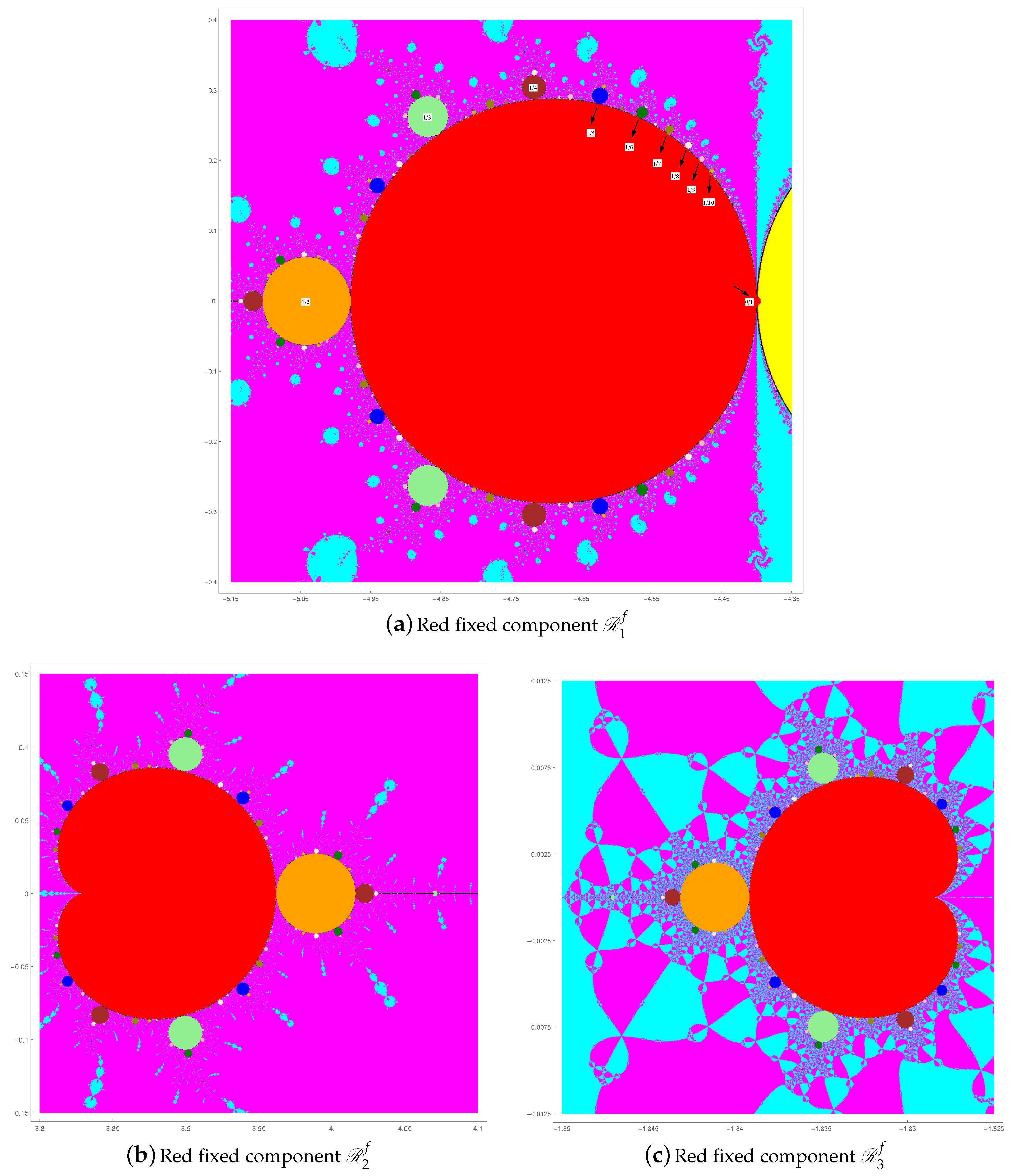
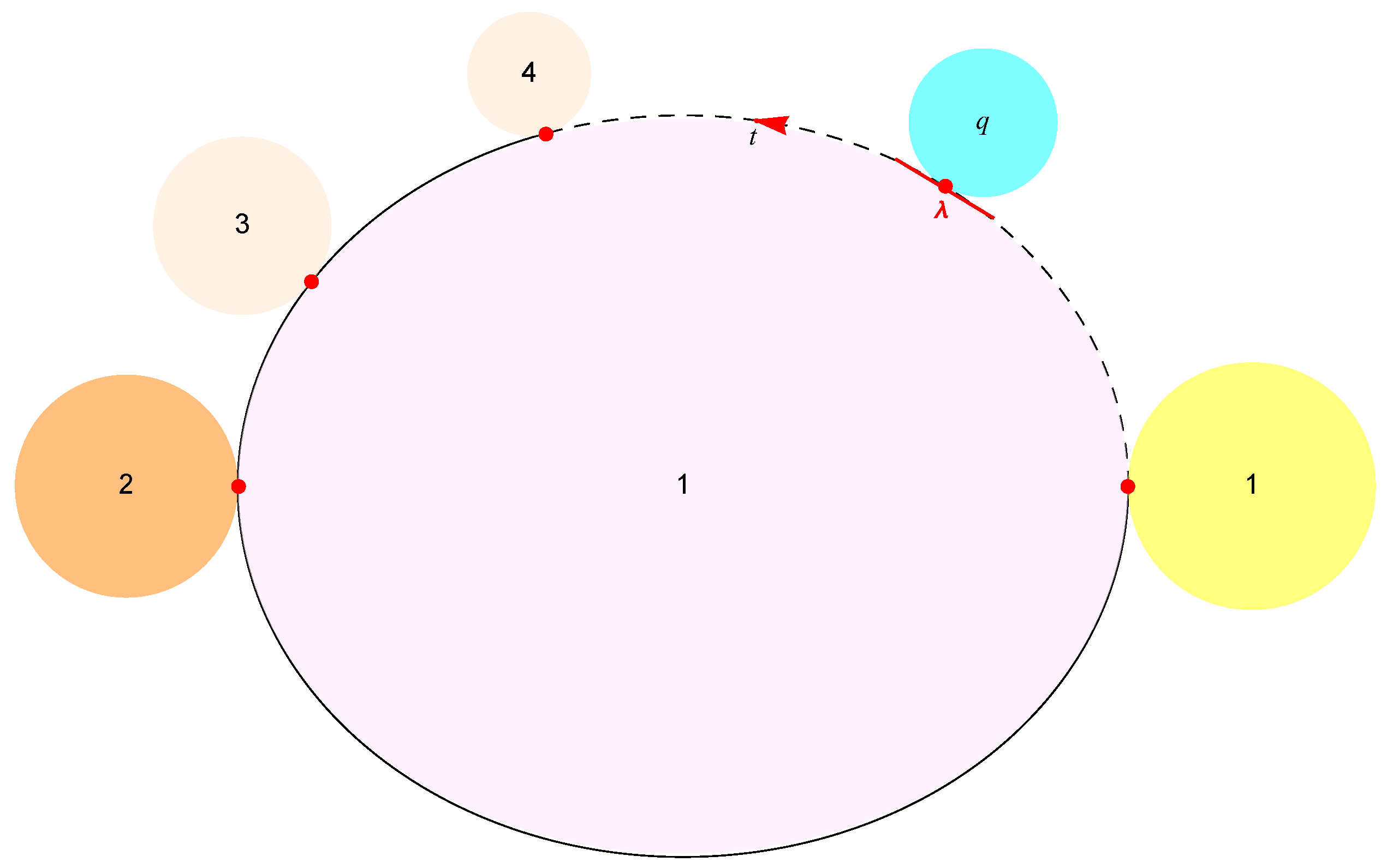
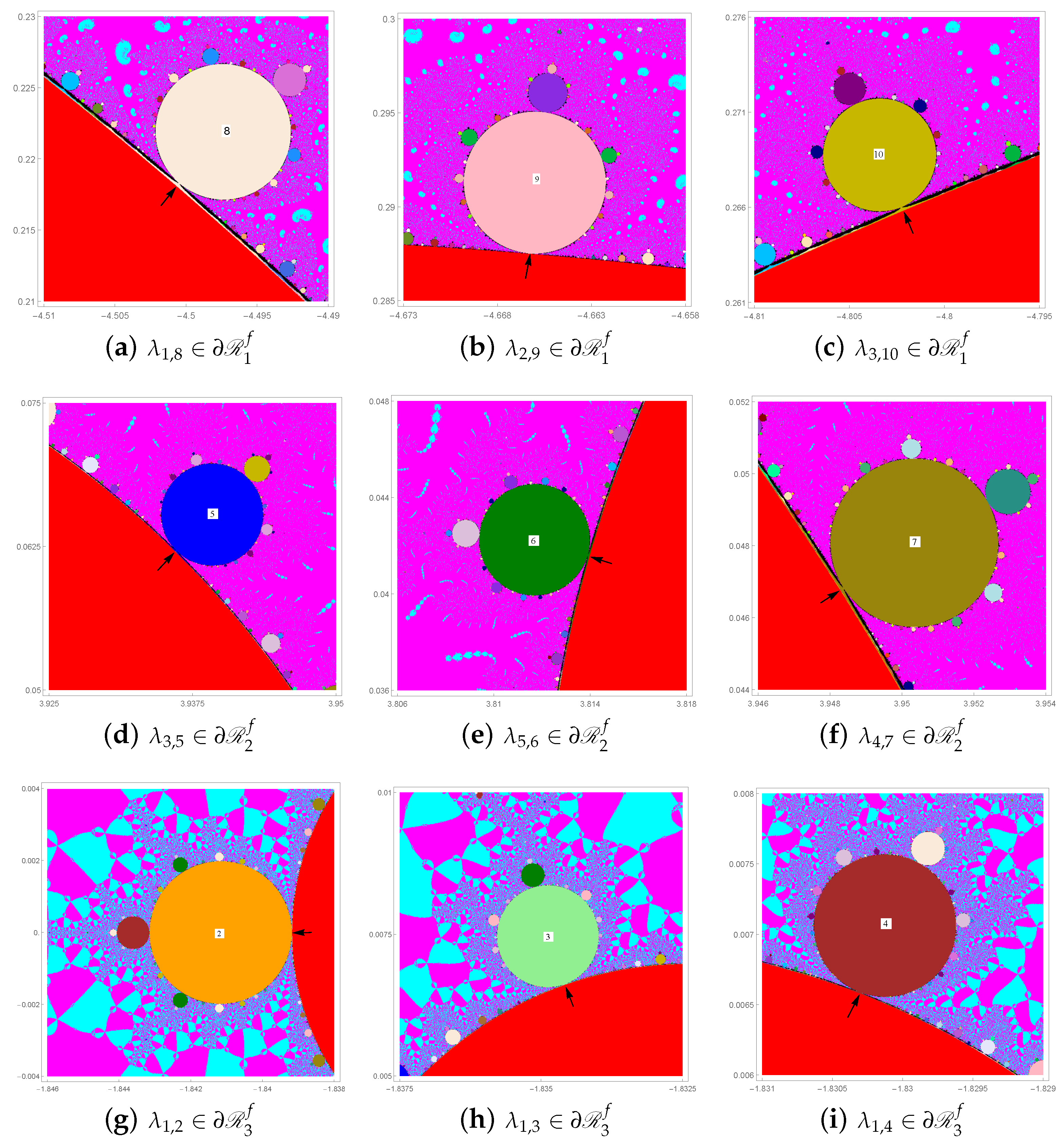
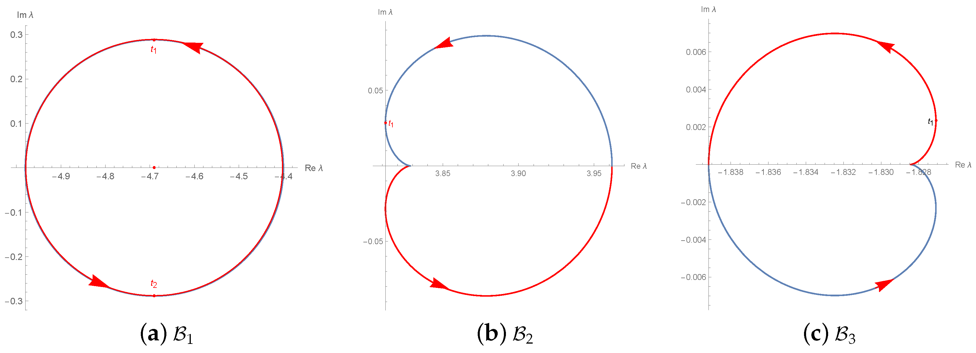
4.2. Bifurcation Points along a Red Fixed Component ${\mathcal{R}}^f$

Suppose that a point $\lambda \left(t\right)$ on a piecewise analytic curve in the complex plane satisfies relation:

$$\lambda \left(t\right)=x\left(t\right)+iy\left(t\right),x,y\in \mathbb{R}\mathrm{for}t\in [t_i,t_f]\subset \mathbb{R}.$$

An exemplary curve consisting of such points $\lambda$ is sketched in Figure 3 along with attracting q-periodic satellite [17] components denoted by $C_q$ and identified by numbers $q\in \mathbb{N}$. Observe that ${\lambda }^{\prime }\left(t\right)=\frac{d\lambda }{dt}$ represents a tangential vector at a parametric location $t\in [t_i,t_f]$. We extensively pursue the case when $\lambda \left(t\right)$ traces a boundary curve of a typical red fixed component ${\mathcal{R}}^f$ as $t\in [t_i,t_f]$ varies. For convenience of notation, we let $\partial {\mathcal{R}}^f$ denote the finite boundary of ${\mathcal{R}}^f$, and write ${\mathcal{F}}_{\lambda }\left(z\right)\equiv \mathcal{F}(\lambda ;z)$ for simple treatment of derivatives.

Let $\lambda$ be an osculating point $\in \partial {\mathcal{R}}^f$ where the $\lambda$-dependent critical orbit of $\mathcal{F}$ approaches an attracting (hyperbolic) q-periodic point $\xi$. We find that the q-periodic point $\xi$ is dependent upon parameter t, since the boundary $\partial {\mathcal{R}}^f$ depends on $t\in [t_i,t_f]$. Hence, we express $\xi =\left|\xi \right|e^{it}$ with $t\in [0,2\pi )$.

Given $q\in \mathbb{N}$, the q-periodic point $\xi$ satisfies the following set of two equations at the common boundary point $\lambda \in \partial {\mathcal{R}}^f\bigcap \partial C_q$ as shown in Figure 3.

$$\left\{\begin{array}{c}{\mathcal{F}}_{\lambda }^q\left(\xi \right)={\mathcal{F}}_{\lambda }\left(\xi \right)=\xi ,\hfill \\ \frac{d}{dz}{\mathcal{F}}_{\lambda }^q{\left(z\right)|}_{z=\xi }={\alpha }^q,\mathrm{with}\alpha ={\mathcal{F}}_{\lambda }^{\prime }\left(\xi \right).\hfill \end{array}\right.$$

(14)

Solving for $\lambda$ from the fixed point relation ${\mathcal{F}}_{\lambda }\left(\xi \left(t\right)\right)=\xi \left(t\right)$ via (4), we are able to obtain:

$$\lambda \left(t\right)=H\left(\xi \left(t\right)\right)=H\left({\mathcal{F}}_{\lambda }^q\left(\xi \left(t\right)\right)\right),$$

(15)

where $H\left(z\right)$ is a rational function in z in view of (4) and differentiable at points except at a finite number of poles. This $\lambda$ will trace a curve in the complex plane as parameter t varies. Hence, by the chain rules, we find the desired derivative at the fixed point $\xi$:

$$\begin{array}{c}\hfill \frac{d\lambda }{dt}=\frac{dH\left(z\right(t\left)\right)}{dz}·\frac{dz}{dt}{|}_{z=\xi }=\frac{dH({\mathcal{F}}_{\lambda }^q\left(z\left(t\right)\right)}{dz}·\frac{dz}{dt}{|}_{z=\xi }=\frac{dH\left(z\right(t\left)\right)}{dz}·{\alpha }^q·\frac{dz}{dt}{|}_{z=\xi },\end{array}$$

(16)

from which we have ${\alpha }^q=1$ in view of the fact that ${\mathcal{F}}_{\lambda }^q\left(\xi \right)=\xi$. Accordingly, Equation (14) reduces to:

$$\left\{\begin{array}{c}{\mathcal{F}}_{\lambda }\left(\xi \right)=\xi ,\hfill \\ \frac{d}{dz}{\mathcal{F}}_{\lambda }^q{\left(z\right)|}_{z=\xi }=1.\hfill \end{array}\right.$$

(17)

Since $\frac{d\lambda }{dt}$ represents a tangent line at a location t, Equation (16) states the common tangent line of $\partial {\mathcal{R}}^f$ and $\partial C_q$. The discussion thus far leads us to the notion of $\ell /q$–bifurcation point below.

Definition 2.

Let$q\in \mathbb{N}$be given. If$\lambda \in \partial {\mathcal{R}}^f\bigcap \partial C_q$and$\alpha \left(\lambda \right)=e^{i2\pi \ell /q}$, with$\ell \in \left\{0,1,2,\cdots ,q-1\right\}$and$(\ell ,q)=1$for$\ell \ne 0$, then λ is called the$\ell /q$–bifurcation point of${\mathcal{R}}^f$or$\ell /q$–root point of$C_q$.

By solving $\alpha \left(\lambda \right)=e^{i2\pi \ell /q}$ for $\lambda$, we are able to find the $\ell /q$-bifurcation point $\lambda ={\lambda }_{\ell ,q}$ in terms of ℓ and q, provided that a set of coprime values of $(\ell ,q)$ are given. If $q=1$ then $\ell =0$ must occur and gives ${\lambda }_{\ell ,q}=1$, which is the fold(saddle-node) bifurcation point in the sense of local bifurcations discussed in Section 2. At this kind of fold bifurcation point, another fixed component different from ${\mathcal{R}}^f$ might arise or the same fixed component as ${\mathcal{R}}^f$ itself merge together due to the connectedness of the component. In the latter case, such a fold bifurcation point ${\lambda }_{\ell ,q}=1$ might be a cusp-like point where ${\mathcal{R}}^f$ itself becomes a primitive component. If $(\ell ,q)=(1,2)$, then ${\lambda }_{\ell ,q}=-1$ becomes the flip (period-doubling) bifurcation point. If $q>2$ and $\ell \ne 0$, then ${\lambda }_{\ell ,q}$ becomes the Neimark-Sacker (secondary Hopf) bifurcation point.

We now conveniently denote the closed boundary curves of ${\mathcal{R}}_i^f$ by ${\mathcal{B}}_i$ for $1\le i\le 3$.

Table 1. Typical ${\lambda }_{\ell ,q}$ along ${\mathcal{B}}_1$ at $t=\frac{2\pi \ell }{q}$, with ${\lambda }_1\left(t\right)$ for $t\in [0,2\pi ]$.

	ℓ
q	0	1	2	3	4	5	6	7	8	9
1	−4.4
2		−4.97983
3		${\left(\begin{array}{c}-4.85312\\ 0.238499\end{array}\right)}^{*}$	$\left(\begin{array}{c}-4.85312\\ -0.238499\end{array}\right)$
4		$\left(\begin{array}{c}-4.71655\\ 0.287269\end{array}\right)$		$\left(\begin{array}{c}-4.71655\\ -0.287269\end{array}\right)$
5		$\left(\begin{array}{c}-4.626\\ 0.281336\end{array}\right)$	$\left(\begin{array}{c}-4.93245\\ 0.158109\end{array}\right)$	$\left(\begin{array}{c}-4.93245\\ -0.158109\end{array}\right)$	$\left(\begin{array}{c}-4.626\\ -0.281336\end{array}\right)$
6		$\left(\begin{array}{c}-4.56717\\ 0.26127\end{array}\right)$				$\left(\begin{array}{c}-4.56717\\ -0.26127\end{array}\right)$
7		$\left(\begin{array}{c}-4.5278\\ 0.239065\end{array}\right)$	$\left(\begin{array}{c}-4.77871\\ 0.27466\end{array}\right)$	$\left(\begin{array}{c}-4.95541\\ 0.115933\end{array}\right)$	$\left(\begin{array}{c}-4.95541\\ -0.115933\end{array}\right)$	$\left(\begin{array}{c}-4.77871\\ -0.27466\end{array}\right)$	$\left(\begin{array}{c}-4.5278\\ -0.239065\end{array}\right)$
8		$\left(\begin{array}{c}-4.50048\\ 0.218276\end{array}\right)$		$\left(\begin{array}{c}-4.90667\\ 0.191651\end{array}\right)$		$\left(\begin{array}{c}-4.90667\\ -0.191651\end{array}\right)$		$\left(\begin{array}{c}-4.50048\\ -0.218276\end{array}\right)$
9		$\left(\begin{array}{c}-4.48088\\ 0.199791\end{array}\right)$	$\left(\begin{array}{c}-4.66632\\ 0.287502\end{array}\right)$		$\left(\begin{array}{c}-4.965\\ 0.0911344\end{array}\right)$	$\left(\begin{array}{c}-4.965\\ -0.0911344\end{array}\right)$		$\left(\begin{array}{c}-4.66632\\ -0.287502\end{array}\right)$	$\left(\begin{array}{c}-4.48088\\ -0.199791\end{array}\right)$
10		$\left(\begin{array}{c}-4.46641\\ 0.183634\end{array}\right)$		$\left(\begin{array}{c}-4.80225\\ 0.265997\end{array}\right)$				$\left(\begin{array}{c}-4.80225\\ -0.265997\end{array}\right)$		$\left(\begin{array}{c}-4.46641\\ -0.183634\end{array}\right)$

${\left(\begin{array}{c}-4.85312\\ 0.238499\end{array}\right)}^{*}\equiv -4.85312+i0.238499,i=\sqrt{-1}$.

,

Table 2. Typical ${\lambda }_{\ell ,q}$ along ${\mathcal{B}}_2$ at $t=\frac{2\pi \ell }{q}$, with ${\lambda }_2\left(t\right)$ for $t\in [0,\pi ]$ and ${\lambda }_3\left(t\right)$ for $t\in (\pi ,2\pi )$.

	ℓ
q	0	1	2	3	4	5	6	7	8	9
1	3.82843
2		3.96186
3		$\left(\begin{array}{c}3.8970\\ -0.0839938\end{array}\right)$	$\left(\begin{array}{c}3.8970\\ 0.0839938\end{array}\right)$
4		$\left(\begin{array}{c}3.84416\\ -0.0776421\end{array}\right)$		$\left(\begin{array}{c}3.84416\\ 0.0776421\end{array}\right)$
5		$\left(\begin{array}{c}3.82177\\ -0.0579666\end{array}\right)$	$\left(\begin{array}{c}3.93609\\ -0.0621221\end{array}\right)$	$\left(\begin{array}{c}3.93609\\ 0.0621221\end{array}\right)$	$\left(\begin{array}{c}3.82177\\ 0.0579666\end{array}\right)$
6		$\left(\begin{array}{c}3.81391\\ -0.041611\end{array}\right)$				$\left(\begin{array}{c}3.81391\\ 0.041611\end{array}\right)$
7		$\left(\begin{array}{c}3.81205\\ -0.0299945\end{array}\right)$	$\left(\begin{array}{c}3.86568\\ -0.0850286\end{array}\right)$	$\left(\begin{array}{c}3.94837\\ -0.0468236\end{array}\right)$	$\left(\begin{array}{c}3.94837\\ 0.0468236\end{array}\right)$	$\left(\begin{array}{c}3.86568\\ 0.0850286\end{array}\right)$	$\left(\begin{array}{c}3.81205\\ 0.0299945\end{array}\right)$
8		$\left(\begin{array}{c}3.81253\\ -0.0219917\end{array}\right)$		$\left(\begin{array}{c}3.9228\\ -0.0728581\end{array}\right)$		$\left(\begin{array}{c}3.9228\\ 0.0728581\end{array}\right)$		$\left(\begin{array}{c}3.81253\\ 0.0219917\end{array}\right)$
9		$\left(\begin{array}{c}3.81382\\ -0.016453\end{array}\right)$	$\left(\begin{array}{c}3.83031\\ -0.0677754\end{array}\right)$		$\left(\begin{array}{c}3.95361\\ -0.0372162\end{array}\right)$	$\left(\begin{array}{c}3.95361\\ 0.0372162\end{array}\right)$		$\left(\begin{array}{c}3.83031\\ 0.0677754\end{array}\right)$	$\left(\begin{array}{c}3.81382\\ 0.016453\end{array}\right)$
10		$\left(\begin{array}{c}3.8153\\ -0.0125579\end{array}\right)$		$\left(\begin{array}{c}3.87498\\ -0.0860643\end{array}\right)$				$\left(\begin{array}{c}3.87498\\ 0.0860643\end{array}\right)$		$\left(\begin{array}{c}3.81530\\ 0.0125579\end{array}\right)$

Red-highlighted values are evaluated at $t\in [0,\pi ]$.

and

Table 3. Typical ${\lambda }_{\ell ,q}$ along ${\mathcal{B}}_3$ at $t=\frac{2\pi \ell }{q}$, with ${\lambda }_3\left(t\right)$ for $t\in [0,\pi ]$ and ${\lambda }_2\left(t\right)$ for $t\in (\pi ,2\pi )$.

	ℓ
q	0	1	2	3	4	5	6	7	8	9
1	−1.82843
2		−1.83917
3		$\left(\begin{array}{c}-1.83458\\ 0.00661529\end{array}\right)$	$\left(\begin{array}{c}-1.83458\\ -0.00661529\end{array}\right)$
4		$\left(\begin{array}{c}-1.83031\\ 0.00658919\end{array}\right)$		$\left(\begin{array}{c}-1.83031\\ -0.00658919\end{array}\right)$
5		$\left(\begin{array}{c}-1.82823\\ 0.0051694\end{array}\right)$	$\left(\begin{array}{c}-1.83742\\ 0.00468664\end{array}\right)$	$\left(\begin{array}{c}-1.83742\\ -0.00468664\end{array}\right)$	$\left(\begin{array}{c}-1.82823\\ -0.0051694\end{array}\right)$
6		$\left(\begin{array}{c}-1.82739\\ 0.00383164\end{array}\right)$				$\left(\begin{array}{c}-1.82739\\ -0.00383164\end{array}\right)$
7		$\left(\begin{array}{c}-1.82712\\ 0.00282147\end{array}\right)$	$\left(\begin{array}{c}-1.83213\\ 0.00697452\end{array}\right)$	$\left(\begin{array}{c}-1.83826\\ 0.00348905\end{array}\right)$	$\left(\begin{array}{c}-1.83826\\ -0.00348905\end{array}\right)$	$\left(\begin{array}{c}-1.83213\\ -0.00697452\end{array}\right)$	$\left(\begin{array}{c}-1.82712\\ -0.00282147\end{array}\right)$
8		$\left(\begin{array}{c}-1.82709\\ 0.00209933\end{array}\right)$		$\left(\begin{array}{c}-1.83648\\ 0.00557375\end{array}\right)$		$\left(\begin{array}{c}-1.83648\\ -0.00557375\end{array}\right)$		$\left(\begin{array}{c}-1.82709\\ -0.00209933\end{array}\right)$
9		$\left(\begin{array}{c}-1.82716\\ 0.0015872\end{array}\right)$	$\left(\begin{array}{c}-1.82906\\ 0.00591232\end{array}\right)$		$\left(\begin{array}{c}-1.83862\\ 0.0027589\end{array}\right)$	$\left(\begin{array}{c}-1.83862\\ -0.0027589\end{array}\right)$		$\left(\begin{array}{c}-1.82906\\ -0.00591232\end{array}\right)$	$\left(\begin{array}{c}-1.82716\\ -0.0015872\end{array}\right)$
10		$\left(\begin{array}{c}-1.82727\\ 0.00122085\end{array}\right)$		$\left(\begin{array}{c}-1.83288\\ 0.00696914\end{array}\right)$				$\left(\begin{array}{c}-1.83288\\ -0.00696914\end{array}\right)$		$\left(\begin{array}{c}-1.82727\\ -0.00122085\end{array}\right)$

Red-highlighted values are evaluated at $t\in [0,\pi ]$.

list typical values of ${\lambda }_{\ell ,q}$ for $1\le q\le 10$ on ${\mathcal{B}}_1$, ${\mathcal{B}}_2$ and ${\mathcal{B}}_3$, respectively and some of them on ${\mathcal{B}}_1$ as well as three of them on each ${\mathcal{B}}_i$ are indicated by arrow lines in Figure 2 and Figure 4. The $0/1$-bifurcation point is the one where the red fixed component is budded from itself or from other fixed component; its location is found to be ${\lambda }_{0,1}=-4.4$ for ${\mathcal{B}}_1$, ${\lambda }_{0,1}=3.82843$ for ${\mathcal{B}}_2$ and ${\lambda }_{0,1}=-1.82843$ for ${\mathcal{B}}_3$. It turns out that ${\mathcal{R}}_2^f$ and ${\mathcal{R}}_3^f$ are respectively regarded as primitive components, while ${\mathcal{R}}_1^f$ is a satellite component budded from a yellow fixed component.

Moreover, coprime pairs of $(\ell ,q)$ give us the number of bifurcation points ${\lambda }_{\ell ,q}$ as the length $\left|{\mathcal{F}}_n\right|$ of the Farey [30] sequence ${\mathcal{F}}_n$ of order n. Theorem 4 in Reference [31] directly gives $\left|{\mathcal{F}}_n\right|$:

$$|{\mathcal{F}}_n|=1+{\displaystyle \sum _{j=1}^n}\varphi \left(j\right),$$

(18)

with $\varphi \left(j\right)$ as Euler’s totient function.

5. Constructing Boundary Equations of Red Fixed Components ${\mathcal{R}}^{\mathit{f}}$

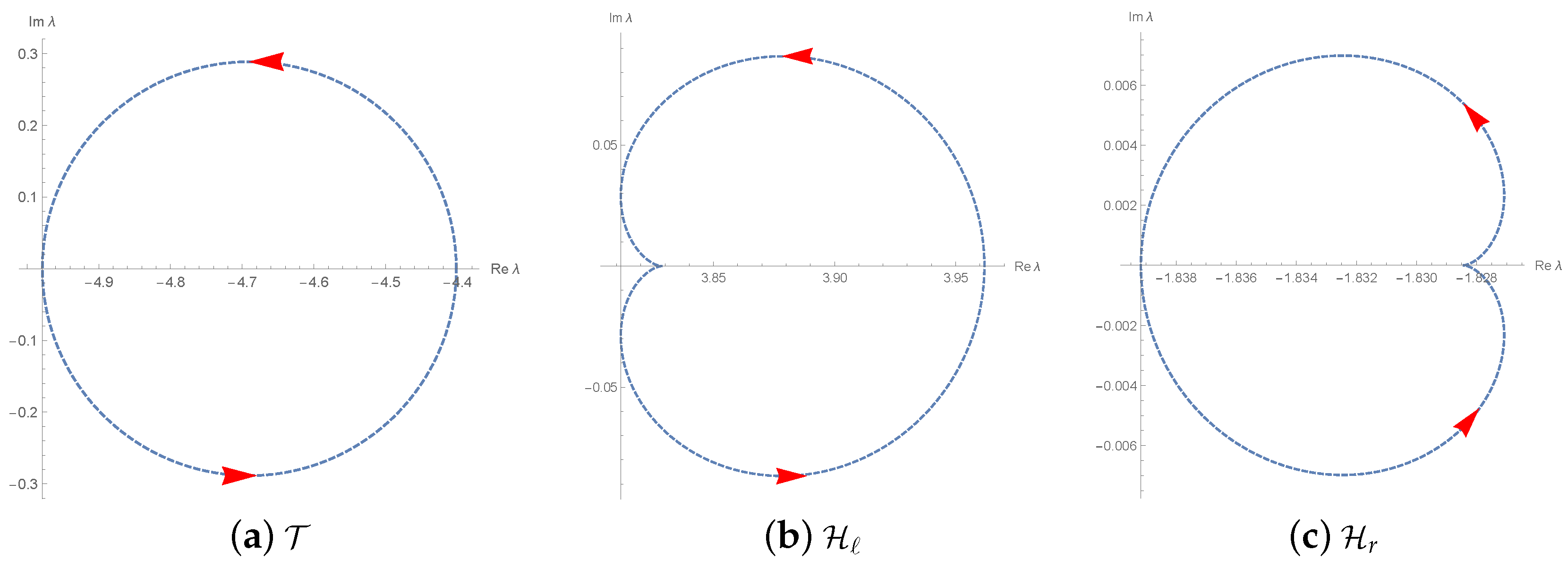
5.1. Establishing Parametric Equations of $\partial {\mathcal{R}}^f$

We establish a boundary equation for such an attracting red fixed component $R_i^f$ associated with a typical $\lambda$-dependent fixed point $\xi$ given by a root of $T(\lambda ;\xi )=0$. During the course of development, we will show the existence of three red fixed components ${\mathcal{R}}^f$, each boundary of which consists of two analytic branches forming a piecewise smooth closed curve. Details of such a boundary curve along with the location of bifurcation points will be discussed in the next section.

Consulting (5) and (6), we find that the fixed point $\xi$ satisfies a set of equations with $\lambda \in \partial {\mathcal{R}}^f$ as follows:

$$\left\{\begin{array}{cc}T(\lambda ;z){|}_{z=\xi }\hfill & ={\displaystyle \prod _{k=1}^2}(z^2+c_{k}z+1){|}_{z=\xi }=0,\hfill \\ \left|\frac{2z^3{(z+1)}^2{Q}_{\lambda }\left(z\right)}{q_{\lambda }{\left(z\right)}^2}\right|\hfill & =|{\mathcal{F}}_{\lambda }^{\prime }\left(z\right){|}_{z=\xi }=1,\hfill \end{array}\right.$$

(19)

where $c_k$ are the two roots being dependent on $\lambda$ from (7); moreover, for preferable algebraic treatments, expressions $Q(\lambda ;z),q(\lambda ;z)$ and $\mathcal{F}(\lambda ;z)$ are written as $Q_{\lambda }\left(z\right),q_{\lambda }\left(z\right)$ and ${\mathcal{F}}_{\lambda }\left(z\right)$ in order. We reconstruct the second equation of (19) with a real parameter $t\in [0,2\pi )$:

$${\mathcal{F}}_{\lambda }^{\prime }\left(z\right){|}_{z=\xi }=\frac{2z^3{(z+1)}^2{Q}_{\lambda }\left(z\right)}{q_{\lambda }{\left(z\right)}^2}{|}_{z=\xi }=e^{it}.$$

(20)

To make notations short, let us write $\xi =z,c_k=c$, and compute $\lambda$ from (7) in terms of c:

$$\lambda =\lambda \left(c\right)=\frac{c^2-5c+8}{c-3}\mathrm{for}c\ne 3,$$

(21)

which defines a branch curve of $\partial {\mathcal{R}}^f$. It is our interest to express $\lambda$ in terms of the parameter t. By use of the symbolic Mathematica commands PolynomialQuotient and PolynomialRemainder described in Section 3.3.4 of Reference [32], we find:

$$\left\{\begin{array}{c}2z^3{(z+1)}^2{Q}_{\lambda }\left(z\right)=(z^2+cz+1)·{\Omega }_q\left(z\right)+{\Omega }_r\left(z\right),\hfill \\ q_{\lambda }{\left(z\right)}^2=(z^2+cz+1)·{\Theta }_q\left(z\right)+{\Theta }_r\left(z\right),\hfill \end{array}\right.$$

(22)

where ${\Omega }_q\left(z\right)$ and ${\Theta }_q\left(z\right)$ are 9- and 6-degree polynomials in order; ${\Omega }_r\left(z\right)=2(18-7c-4c^2+c^3)\delta \left(z\right)$ and ${\Theta }_r\left(z\right)=-4(c-2)\delta \left(z\right)$ with $\delta \left(z\right)={\left(\frac{c-2}{c-3}\right)}^2\left[c^3-2c+(1-3c^2+c^4)z\right]$.

Due to the fact that $(z^2+cz+1)=0$, relation (20) directly yields:

$${\mathcal{F}}_{\lambda }^{\prime }\left(\xi \right)=\frac{{\Omega }_r\left(z\right)}{{\Theta }_r\left(z\right)}=-\frac{c^3-4c^2-7c+18}{2(c-2)}=e^{it},0\le t<2\pi ,c\ne 2,$$

(23)

where $c=c_k$ for $k\in \{1,2\}$ can be expressed in terms of $\lambda$ from (7). Since ${\mathcal{F}}_{\lambda }^{\prime }\left(\xi \right)$ is not explicitly dependent on fixed points $\xi$ themselves but only on coefficient c, the stabilities of all four fixed points $\xi$ found from $T(\lambda ;\xi )=0$ remain equal to one another. This kind of favorable dependence on c clearly reduces the possible lengthy algebraic work required for each fixed point.

Evidently, three roots $C_1\left(t\right),C_2\left(t\right),C_3\left(t\right)$ of $c=c_k\left(t\right)$ can be found for each $k\in \{1,2\}$ in terms of $t\in [0,2\pi )$ from the cubic equation of (23):

$$\left\{\begin{array}{c}{C}_1\left(t\right)=\frac{1}{3}\left(4-\sigma -\frac{37-6e^{it}}{\sigma }\right),\hfill \\ C_2\left(t\right)=\frac{1}{6}\left(8+\sigma (1-i\sqrt{3})+\frac{(1+i\sqrt{3})(37-6e^{it})}{\sigma }\right),\hfill \\ C_3\left(t\right)=\frac{1}{6}\left(8+\sigma (1+i\sqrt{3})+\frac{(1-i\sqrt{3})(37-6e^{it})}{\sigma }\right),\hfill \end{array}\right.$$

(24)

with $\sigma ={\left(53-18e^{it}+3\sqrt{6}\sqrt{-886+421e^{it}-68e^{2it}+4e^{3it}}\right)}^{1/3}$.

Further refined computations readily offer:

$$\left\{\begin{array}{ccc}\overline{C_1\left(t\right)}\hfill & =C_1(2\pi -t),\hfill & \mathrm{for}t\in [0,\pi ],\hfill \\ \overline{C_2(\pi +t)}\hfill & =C_3(2\pi -t),\hfill & \mathrm{for}t\in (0,\pi ),\hfill \\ \overline{C_3(\pi -t)}\hfill & =C_2(2\pi -t),\hfill & \mathrm{for}t\in (0,\pi ),\hfill \end{array}\right.$$

(25)

where $\overline{\eta }$ reveals the complex conjugate of $\eta$. We say the points t at which a complex function $f\left(z\right)$ is not analytic on $\mathbb{C}$ are called singular points or singularities of $f\left(z\right)$. Preferably, the continuity relations hold at the singular points $t=0$ and $t=\pi$:

$$C_2\left(0\right)=C_3\left(2{\pi }_{-}\right),C_2\left(\pi \right)=C_3\left({\pi }_{+}\right),C_3\left(0\right)=C_2\left(2{\pi }_{-}\right),C_3\left(\pi \right)=C_2\left({\pi }_{+}\right),$$

(26)

where $a_{+}$ and $b_{-}$ imply the respective limits from the above of a and the below of b.

In view of (21) and (24), we can express three $\lambda$-values at $C_1\left(t\right),C_2\left(t\right)$ and $C_3\left(t\right)$. Denoting ${\lambda }_j\left(t\right)=\lambda \left(C_j\left(t\right)\right)$ for $t\in [0,2\pi )$ leads us to the parametric expression for each $j\in \{1,2,3\}$ as follows:

$$\left\{\begin{array}{c}{\lambda }_1\left(t\right)=-\frac{{\mu }^2+5\mu +8}{\mu +3},\mu =\frac{37-e^{it}-4\sigma +{\sigma }^2}{3\sigma },\hfill \\ {\lambda }_2\left(t\right)=\frac{1}{12}\left[-8+(1-i\sqrt{3})(2\sigma -\tau )-\frac{72(1+i\sqrt{3})}{5(1+i\sqrt{3})-2\sigma +\tau }\right],\tau =\frac{(1-i\sqrt{3})(37-6e^{it})}{\sigma },\hfill \\ {\lambda }_3\left(t\right)=\frac{288-30\rho +{\rho }^2}{6(\rho -18)},\rho =\sigma (1+i\sqrt{3})+\tau +8.\hfill \end{array}\right.$$

(27)

The result of Equation (27) suggests that the number of the red fixed components is three and enables us to construct the three boundaries of ${\mathcal{R}}^f$ parametrically as $t\in [0,2\pi )$ varies. Indeed, $C_j\left(t\right)$ and $\lambda \left(C_j\left(t\right)\right)$ have also singular points at $t=0$ and $t=\pi$.

Since ${\lambda }_k\left(t\right)$ in (21) is a function of c which is piecewise analytic with such singularities, we shall have same properties given by (25) and (26) with letter $C_j$ replaced by ${\lambda }_j$. In light of this observation along with the symmetry of $\mathcal{P}$, we characterize the three closed boundary curves ${\mathcal{B}}_j$ of ${\mathcal{R}}^f$ as ${\mathcal{B}}_j=\{{\beta }_j\left(t\right),t\in [0,2\pi )\}$ for $(1\le j\le 3)$, with

$${\beta }_1\left(t\right)={\lambda }_1\left(t\right)\mathrm{for}t\in [0,2\pi ),{\beta }_2\left(t\right)=\left\{\begin{array}{c}{\lambda }_2\left(t\right),t\in [0,\pi ],\hfill \\ {\lambda }_3\left(t\right),t\in (\pi ,2\pi ),\hfill \end{array}\right.{\beta }_3\left(t\right)=\left\{\begin{array}{c}{\lambda }_3\left(t\right),t\in [0,\pi ],\hfill \\ {\lambda }_2\left(t\right),t\in (\pi ,2\pi ).\hfill \end{array}\right.$$

(28)

Any of ${\beta }_j\left(t\right)$ is generally comprised of piecewise analytic arcs with singularities at $t=0$ and $t=\pi$. The functions ${\beta }_j\left(t\right),(1\le j\le 3)$ are plotted for $t\in [0,2\pi )$ in Figure 5. Let ${\mathcal{B}}_j$ be a closed plane curve traced by ${\beta }_j\left(t\right)$ for $t\in [0,2\pi )$, which represents the boundary of j-th red fixed component ${\mathcal{R}}_j^f$. The symmetry of $\mathcal{P}$ clearly reflects the symmetry of ${\mathcal{B}}_j$ with respect to the horizontal axis. The blue arcs correspond to ones with $t\in [0,\pi ]$.

5.2. Geometric Features of Boundaries ${\mathcal{B}}_j$

In this section, various typical geometric features, including curvatures, perimeters and bounding areas of the closed boundary curves ${\mathcal{B}}_j$, will be treated from a perspective of Euclidean planar curves. Let $x_j\left(t\right)=\Re \left({\lambda }_j\left(t\right)\right)$ and $y_j\left(t\right)=\Im \left({\lambda }_j\left(t\right)\right)$ respectively denote the real and imaginary part of ${\lambda }_j\left(t\right)$. By elaborate computing with approximately 10 digits of accuracy, we obtain the arc lengths of ${\mathcal{B}}_j$:

$$\begin{array}{c}|\stackrel{◠}{{\mathcal{B}}_1}|={\int }_0^{2\pi }\sqrt{x_1^{\prime }{\left(t\right)}^2+y_1^{\prime }{\left(t\right)}^2}dt\approx 1.8170393896,\hfill \\ |\stackrel{◠}{{\mathcal{B}}_2}|={\int }_0^{\pi }\sqrt{x_2^{\prime }{\left(t\right)}^2+y_2^{\prime }{\left(t\right)}^2}dt+\underset{ϵ\to 0}{\lim }{\int }_{\pi +ϵ}^{2\pi -ϵ}\sqrt{x_3^{\prime }{\left(t\right)}^2+y_3^{\prime }{\left(t\right)}^2}dt\approx 0.5312573924,\hfill \\ |\stackrel{◠}{{\mathcal{B}}_3}|={\int }_0^{\pi }\sqrt{x_3^{\prime }{\left(t\right)}^2+y_3^{\prime }{\left(t\right)}^2}dt+\underset{ϵ\to 0}{\lim }{\int }_{\pi +ϵ}^{2\pi -ϵ}\sqrt{x_2^{\prime }{\left(t\right)}^2+y_2^{\prime }{\left(t\right)}^2}dt\approx 0.04299949400,\hfill \end{array}$$

(29)

as well as the bounding area $A_j$ enclosed by ${\mathcal{B}}_j$:

$A_1=2{\int }_0^{\pi }{y}_2\left(t\right)x_2^{\prime }\left(t\right)dt\approx 0.262733068875$.

$A_2=2\left(\left|{\int }_{t_1}^{\pi }{y}_2\left(t\right)x_2^{\prime }\left(t\right)dt\right|-|{\int }_0^{t_1}{y}_2\left(t\right)x_2^{\prime }\left(t\right)dt|\right)\approx 0.020812361489$, with $t_1=0.87751899915$.

$A_3=2|{\int }_{t_1}^{\pi }{y}_3\left(t\right)x_3^{\prime }\left(t\right)dt-{\int }_0^{t_1}{y}_3\left(t\right)x_3^{\prime }\left(t\right)dt|\approx 0.00013612636360$, with $t_1=0.822062652525$.

The curvatures of ${\mathcal{B}}_j$ calculated when $t=\frac{\pi }{4},\frac{\pi }{3},\frac{\pi }{2},\frac{2\pi }{3},\frac{3\pi }{4}$, and the average curvatures are shown in

Table 4. Some Geometric characteristics of Plane Curves ${\mathcal{B}}_i$ and $\mathcal{T}$, ${\mathcal{H}}_{\ell }$ and ${\mathcal{H}}_r$.

	GP	${\mathit{A}}_{\mathit{b}}$:	${\mathit{L}}_{\mathit{p}}$:	$\mathit{\kappa }\left(\mathit{t}\right)$: Curvature
PC		Bounding Area	Perimeter	$\frac{\mathit{\pi }}{\mathbf{4}}$	$\frac{\mathit{\pi }}{\mathbf{3}}$	$\frac{\mathit{\pi }}{\mathbf{2}}$	$\frac{\mathbf{2}\mathit{\pi }}{\mathbf{3}}$	$\frac{\mathbf{3}\mathit{\pi }}{\mathbf{4}}$	$\overline{\mathit{\kappa }}$
${\mathcal{B}}_1$		0.2627330688	1.8170393896	3.44989	3.43720	3.43430	3.4522	3.46289	3.44730
$\mathcal{T}$		0.2614338703	1.8125327322	3.46652	3.46652	3.46652	3.46652	3.46652	3.46652
${\mathcal{B}}_2$		0.02081236148	0.5312573924	24.98557	19.53529	14.53345	12.47003	11.92695	16.69026
${\mathcal{H}}_{\ell }$		0.02097440675	0.5337209668	12.16806	12.98094	15.89834	22.48365	29.37631	18.58150
${\mathcal{B}}_3$		0.0001361263636	0.04299949400	289.93697	229.64877	174.87643	152.23274	146.18980	198.57694
${\mathcal{H}}_r$		0.0001360364744	0.04298303774	364.76611	279.17989	197.40999	161.18458	151.09107	230.72633

GP: Geometric properties, PC: Plane curves, $\overline{\kappa }$: Mean value of $\kappa$.

. In addition, the bounding areas and perimeters are listed together with them in Table 4. The following lemma immediately follows from the geometric properties listed in Table 4.

Lemma 3.

The shapes of boundary curves${\mathcal{B}}_i$have the following characterizations.

(i) ${\mathcal{B}}_1$ is not a circle. (ii) Neither ${\mathcal{B}}_2$ nor ${\mathcal{B}}_3$ is a cardioid.

Remark 3.

Consider a circle$\mathcal{T}=\{(a_c+r_c\cos t,r_c\sin t),t\in [0,2\pi )\}$osculating at the topmost point$(a_c,r_c)$of${\mathcal{B}}_1$, with$a_c=-4.6900936467$, and$r_c=0.28847354384$. Let${\rho }_1\left(t\right)=|{\beta }_1\left(t\right)-a_c|$be the distance from the center$(a_c,0)$of$\mathcal{T}$to a point${\beta }_1\left(t\right)$at a location t. Then by elaborate computations, we have${\rho }_1\left(t\right)\ge r_c$for all$t\in [0,2\pi )$and find$\mathcal{T}$is completely inscribed in${\mathcal{B}}_1$.

Let us define two cardioids${\mathcal{H}}_{\ell }=\{(a_{\ell }+{\rho }_{\ell }(1+\cos t)\cos t,{\rho }_{\ell }(1+\cos t)\sin t),t\in [0,2\pi )\}$and${\mathcal{H}}_r=\{(a_r+{\rho }_r(1-\cos t)\cos t,{\rho }_r(1-\cos t)\sin t),t\in [0,2\pi )\}$, where$a_{\ell }=3.82842712474,{\rho }_{\ell }=0.066715120853,a_r=-1.82842712474,{\rho }_r=0.0053728797175$. In view of geometric properties in Table 4,${\mathcal{H}}_{\ell }$and${\mathcal{H}}_r$respectively resemble${\mathcal{B}}_2$and${\mathcal{B}}_3$with exactly the same diametral chords. The curves of$\mathcal{T}$,${\mathcal{H}}_{\ell }$and${\mathcal{H}}_r$are evidently shown in Figure 6.

6. Conclusions

In the previous study in Reference [13], the only yellow fixed component related to $\lambda$-free strange fixed point $z=1$ had a circle as its boundary curve, which described branching phenomena without difficulties. On the other hand, in the present study, the formation of the red fixed component ${\mathcal{R}}^f$ is more complicated because the strange fixed point $z=z\left(\lambda \right)$ (given by the roots of degree-4 polynomial $T(\lambda ;z)$ in (6)) depends on $\lambda$, and thus the analysis of the desired bifurcation phenomena requires a higher level of tools. One such tool is to introduce a suitable parameter, say, t, to represent a curve on the complex plane. The expression $\lambda \left(t\right)=x\left(t\right)+iy\left(t\right)$, given at the beginning of Section 4.2, will be very helpful in describing the branching phenomena occurring in the $\lambda$-parameter plane $\mathcal{P}$. In particular, it has enabled us to draw some geometric properties of ${\mathcal{R}}^f$ observed in $\mathcal{P}$.

Through the Möbius-conjugacy map applied to $f\left(z\right)={(z-a)}^m{(z-b)}^m$, we have studied the long-term orbit behavior of a $\lambda$-family of fourth-order multiple-root finders in $\mathcal{P}$. We have theoretically formulated the boundary equation of the red fixed hyperbolic component ${\mathcal{R}}^f$, by representing a point $\lambda \left(t\right)$ with parameter $t\in [0,2\pi )$. The boundaries of ${\mathcal{R}}^f$ have not turned out to be known geometric figures. In fact, they have proven to be neither circles nor cardioids. The number of ${\mathcal{R}}^f$ is 3 higher than that of the yellow fixed component studied in Reference [13]. Equating the derivative of a q-periodic point to that of a $\lambda$-dependent fixed point at the common osculating point $\lambda$ between ${\mathcal{R}}^f$ and q-periodic components have induced the relation ${{{\mathcal{F}}_{\lambda }}^{\prime }\left(\xi \right)}^q=1$, which has enabled us to successfully locate the bifurcation points ${\lambda }_{\ell ,q}$ directly from ${{\mathcal{F}}_{\lambda }}^{\prime }\left(\xi \right)=e^{i2\pi \ell /q}$ with ℓ and q defined in Definition 2. With $\lambda$ selected in the magenta or cyan region of $\mathcal{P}$, iterative scheme $W_f$ in (2) stably converges to the desired root. However, members of the family with $\lambda$ selected in other regions would exhibit unfavorable numerical behavior.

According to Proposition 1-a, $T(\lambda ;z)$ is composed of factors of the form $(z^2+c_{k}z+1)$ for $k=1,2,\cdots$. Therefore, if the order of the governing equation (for instance, (7)) for the coefficients $c_k$ is not greater than 4, that is, the order of $T(\lambda ;z)$ is not greater than 8, then it is possible to find the exact $\lambda$-dependent strange fixed point $z=z\left(\lambda \right)$. Otherwise, the bifurcation phenomena will be resolved neither theoretically nor computationally. As our future study, we will challenge to investigate the bifurcation phenomena of the period-2 orange components shown in Figure 2 and locate the desired global bifurcation points by a theoretical formulation of the desired boundary equation, provided the order of $T(\lambda ;z)$ is hopefully not greater than 8.

References

1. Behl, R.; Cordero, A.; Motsa, S.; Torregrosa, J. On developing fourth-order optimal families of methods for multiple roots and their dynamics. Appl. Math. Comput. 2015, 265, 520–532. [Google Scholar] [CrossRef] [Green Version]
2. Behl, R.; Cordero, A.; Motsa, S.; Torregrosa, J.; Kanwar, V. An optimal fourth-order family of methods for multiple roots and its dynamics. Numer. Algorithms 2016, 11, 775–796. [Google Scholar] [CrossRef]
3. Geum, Y.H.; Kim, Y.I. A two-parameter family of fourth-order iterative methods with optimal convergence for multiple zeros. J. Appl. Math. 2013, 369067, 1–7. [Google Scholar]
4. Neta, B.; Scott, M.; Chun, C. Basin attractors for various methods for multiple roots. Appl. Math. Comput. 2012, 218, 5043–5066. [Google Scholar] [CrossRef]
5. Geiser, J. A multiple iterative splitting method for higher order differential equations. J. Math. Anal. Appl. 2015, 424, 1447–1470. [Google Scholar] [CrossRef]
6. Hosseini, R.; Tatari, M. Some splitting methods for hyperbolic PDEs. Appl. Numer. Math. 2019, 146, 361–378. [Google Scholar] [CrossRef]
7. Gao, J.; Liang, H.; Ma, S. Strong convergence of the semi-implicit Euler method for nonlinear stochastic Volterra integral equations with constant delay. Appl. Math. Comput. 2019, 348, 385–398. [Google Scholar] [CrossRef]
8. González-Pinto, S.; Hernández-Abreu, D. Semi-implicit methods for differential systems with semi-stable equilibria. Appl. Numer. Math. 2006, 56, 210–221. [Google Scholar] [CrossRef]
9. L-Jawary, M.A.A.; Azeez, M.M.; Radhi, G.H. Analytical and Numerical Solutions for the Nonlinear Burgers and Advection–Diffusion Equations by Using a Semi-Analytical Iterative Method. Comput. Math. Appl. 2018, 76, 155–171. [Google Scholar] [CrossRef]
10. Campos, B.; Cordero, A.; Torregrosa, J.R.; Vindel, P. Orbits of period two in the family of a multipoint variant of Chebyshev-Halley family. Numer. Algorithms 2016, 73, 141–156. [Google Scholar] [CrossRef] [Green Version]
11. Kung, H.T.; Traub, J.F. Optimal order of one-point and multipoint iteration. J. Assoc. Comput. Mach. 1974, 21, 643–651. [Google Scholar] [CrossRef]
12. Ahlfors, L.V. Complex Analysis; McGraw-Hill Book, Inc.: New York, NY, USA, 1979. [Google Scholar]
13. Geum, Y.H.; Kim, Y.I. Long-term orbit dynamics viewed through the yellow main component in the parameter space of a family of optimal fourth-order multiple-root finders. Discret. Contin. Dyn. Syst. Ser. B 2020, 22. [Google Scholar] [CrossRef] [Green Version]
14. Hale, J.; Koçak, H. Dynamics and Bifurcations; Springer: New York, NY, USA, 1991. [Google Scholar]
15. Thompson, J.M.T.; Stewart, H.B. Nonlinear Dynamics and Chaos; John Wieley & Sons Ltd.: New York, NY, USA, 1986. [Google Scholar]
16. Carleson, L.; Gamelin, T.W. Complex Dynamics; Springer: New York, NY, USA, 1993. [Google Scholar]
17. Peitgen, H.; Richter, P. The Beauty of Fractals; Springer: New York, NY, USA, 1986. [Google Scholar]
18. Blanchard, P. The dynamics of Newton’s method. In Proceedings of Symposia in Applied Mathematics; American Mathematical Society: Providence, RI, USA, 1994; Volume 49, pp. 139–154. [Google Scholar]
19. Beardon, A.F. Iteration of Rational Functions; Springer: New York, NY, USA, 1991. [Google Scholar]
20. Lee, M.-Y.; Kim, Y.I. Bifurcations along the Boundary Curves of Red Fixed Components in the Parameter Space for Uniparametric, Jarratt-Type Simple-Root Finders. Mathematics 2020, 8, 51. [Google Scholar] [CrossRef] [Green Version]
21. Devaney, R.L. An Introduction to Chaotic Dynamical Systems; Addison-Wesley Publishing Company, Inc.: New York, NY, USA, 1987. [Google Scholar]
22. Nayfeh, A.H.; Balachandran, B. Applied Nonlinear Dynamics: Analytical, Computational, and Experimental Methods; John Wiley & Sons: New York, NY, USA, 2008. [Google Scholar]
23. Argyros, I.K.; Magreñán, Á.A. On the convergence of an optimal fourth-order family of methods and its dynamics. Appl. Math. Comput. 2015, 252, 336–346. [Google Scholar] [CrossRef]
24. Behl, R.; Cordero, A.; Motsa, S.; Torregrosa, J. Multiplicity anomalies of an optimal fourth-order class of iterative methods for solving nonlinear equations. Nonlinear Dyn. 2018, 91, 98–112. [Google Scholar] [CrossRef] [Green Version]
25. Chun, C.; Neta, B.; Kim, S. On Jarratt’s family of optimal fourth-order iterative methods and their dynamics. Fractals 2014, 22, 1450013. [Google Scholar] [CrossRef] [Green Version]
26. García-Olívo, M.; Gutíerrez, J.M.; Magreñán, Á.A. A complex dynamical approach of Chebyshev’s method. SeMA J. 2015, 71, 57–68. [Google Scholar] [CrossRef]
27. Magreñán, Á.A. Different anomalies in a Jarratt family of iterative root-finding methods. Appl. Math. Comput. 2014, 233, 29–38. [Google Scholar]
28. Chicharro, F.; Cordero, A.; Torregrosa, J.R. Drawing Dynamical and Parameters Planes of Iterative Families and Methods. Sci. World J. 2013, 2013, 1–11. [Google Scholar] [CrossRef]
29. Geum, Y.H.; Kim, Y.I.; Magreñán, Á.A. A study of dynamics via Mobius conjugacy map on a family of sixth-order modified Newton-like multiple-zero finders with bivariate polynomial weight functions. J. Comput. Appl. Math. 2018, 344, 608–623. [Google Scholar] [CrossRef]
30. Ainsworth, J.; Dawson, M.; Pianta, J.; Warwick, J. The Farey Sequence. 2012. Available online: http://www.maths.ed.ac.uk/~aar/fareyproject.pdf (accessed on 24 January 2020).
31. Geum, Y.H.; Kim, Y.I. On Locating and Counting Satellite Components Born along the Stability Circle in the Parameter Space for a Family of Jarratt-Like Iterative Methods. Mathematics 2019, 7, 839. [Google Scholar] [CrossRef] [Green Version]
32. Wolfram, S. The Mathematica Book, 5th ed.; Wolfram Media: Champaign, IL, USA, 2003. [Google Scholar]
Figure 1. Parameter space P with three red fixed components R i f , ( 1 i 3 ) .
Mathematics 08 00763 g001
Figure 2. Three Red fixed components R i f , ( 1 i 3 ) .
Mathematics 08 00763 g002
Figure 3. Bifurcation geometry along the boundary of a typical fixed component.
Mathematics 08 00763 g003
Figure 4. Typical bifurcation points λ , q of q-periodic components occurring on R j f .
Mathematics 08 00763 g004
Figure 5. Boundary curves of the three red fixed components R f .
Mathematics 08 00763 g005
Figure 6. Plane curves T , H and H r closely resembling the boundaries of red-fixed components R f .
Mathematics 08 00763 g006