Bifurcations along the Boundary Curves of Red Fixed Components in the Parameter Space for Uniparametric, Jarratt-Type Simple-Root Finders

Abstract

Bifurcations have been studied with an extensive analysis of boundary curves of red, fixed components in the parametric space for a uniparametric family of simple-root finders under the Möbius conjugacy map applied to a quadratic polynomial. An elementary approach from the perspective of a plane curve theory properly describes the geometric figures resembling a circle or cardioid to characterize the underlying boundary curves that are parametrically expressed. Moreover, exact bifurcation points for satellite components on the boundaries have been found, according to the fact that the tangent line at a bifurcation point simultaneously touches the red fixed component and the satellite component. Computational experiments implemented with examples well reflect the significance of the theoretical backgrounds pursued in this paper.

1. Introduction

Iterative root-finding approximate methods naturally arise due to the infeasibility of the exact methods under general circumstances to solve the nonlinear governing equations frequently encountered in the fields of social and engineering sciences. Newton’s method has been widely accepted in view of its simplicity and quadratic convergence. Development of higher-order iterative root-finding schemes [1,2,3,4,5,6,7,8] has been a primary topic among the scholars and researchers working in this area.

Recently, an optimal family of fourth-order simple-root finders locating a zero of $f\left(x\right)\in {\mathbb{C}}^m$ have been studied by Cordero et al. [9] in the form:

$$\left\{\begin{array}{c}{y}_n=x_n-\frac{2}{3}·{f^{\prime }\left(x_n\right)}^{-1}f\left(x_n\right),\hfill \\ x_{n+1}=x_n-H\left(t\right){f^{\prime }\left(x_n\right)}^{-1}f\left(x_n\right),\mathrm{with}t={f^{\prime }\left(x_n\right)}^{-1}{f}^{\prime }\left(y_n\right),\mathrm{for}n\in \mathbb{N}\cup \left\{0\right\},\hfill \end{array}\right.$$

(1)

where $f:D\subseteq {\mathbb{C}}^m\to {\mathbb{C}}^m$ has a zero $\alpha \in D$ and is holomorphic [10,11] in a region containing $\alpha$; H is a matrix function defined on ${\mathbb{C}}^{m\times m}$.

When $m=1$ and $H\left(t\right)=\frac{1}{2}{(3t-1)}^{-1}(3t+1)$, iterative scheme (1) reduces to so-called Jarratt’s method for a single scalar equation $f\left(x\right)=0\in \mathbb{C}$.

An iterative scheme can be regarded as a discrete dynamical system, by treating the iteration index as the time-evolving variable. The iterative solution process indeed implies the investigation of the long-term behavior underlying the dynamical system. For a single scalar equation with

$$m=1,H\left(t\right)=\frac{23}{8}-3t+\frac{9}{8}{t}^2+\frac{\lambda }{6}{(t-1)}^3\mathrm{and}\lambda \in \mathbb{C},$$

(2)

Cordero et al. [9] have presented some dynamical aspects on the Riemann sphere $\overline{\mathbb{C}}$ for the conjugated map via Möbius conjugacy [12] map $M\left(z\right)=\frac{z-a}{z-b},(a\ne b)$ with $f\left(z\right)=(z-a)(z-b)$ in the $\lambda$-parameter space, a detailed analysis of which has been strengthened by Geum-Kim [13].

To characterize such dynamical aspects underlying the long-term behavior of iterative scheme (1), we concentrate our current analysis on the study of geometric properties of the boundary curves of attracting red fixed components shown in Figure 1, for a $\lambda$-value selected in which the corresponding critical orbit attracts to a $\lambda$-dependent fixed point. In addition, we focus on the location of bifurcation points of satellite or primitive components [14] budded along the boundaries.

Further analyses, investigations and developments are pursued in the remaining sections. Section 2 describes preliminary studies on orbit behavior, perturbational stability and bifurcations occurring on the stability unit circle [13]. Section 3 discusses some properties of the fixed and critical points of the conjugated map. Section 4 deals with the parameter space and the long-term behavior of a critical orbit under the conjugated map. Besides, governing equations for locating and counting bifurcation points are established based on an elementary theory of plane curves and the Farey [15] sequence. Section 5 explores theoretical backgrounds for developing parametric boundary equations and the location of bifurcation points occurring along the boundaries. In the final section, we summarize overall current developments and propose the forthcoming exploration.

2. Preliminary Studies

2.1. Orbit Behavior

Perceiving the notion of conjugacy h [16,17] between two dynamical systems F and G, we follow invariances of topological and diffeomorphic conjugacies from Theorem 2.1 of [17]. Furthermore, we find an isomorphism between the orbits of F and G that behaves similarly under h, in view of the fact that the two n-fold compositions $F^n$ and $G^n$ satisfy the relation $F^n=h\circ G^n\circ h^{-1}$ for any integer n.

Lemma 1.

Assume that $f:\mathsf{\Omega }\subseteq \overline{\mathbb{C}}\to \mathsf{\Omega }$ is analytic [10] on Ω and has a fixed point $\xi \in \mathsf{\Omega }$ satisfying $|f^{\prime }\left(\xi \right)|<1$. Then the sequence ${\{z_{n+1}=f\left(z_n\right)\}}_0^{\infty }$ converges to a unique fixed point ξ for given $z_0\in \mathsf{\Omega }$.

Proof. 

The property of being analytic at $\xi$ allows us to write

$$z_{n+1}-\xi =f\left(z_n\right)-f\left(\xi \right)=(z_n-\xi )(f^{\prime }\left(\xi \right)+\eta ),$$

(3)

where $\eta \to 0$ as $z_n\to \xi$. We now choose a sufficiently large integer $N>0$ and a constant $\beta >0$ such that $|f^{\prime }\left(\xi \right)|+|\eta |=\beta <1$ whenever $n\ge N$. Then, for any $k\in \mathbb{N}\cup \left\{0\right\}$,

$$|z_{N+k+1}-\xi |=|f(z_{N+k}-f\left(\xi \right)|=|z_{N+k}-\xi \left|\right|f^{\prime }\left(\xi \right)+\eta |\le |z_{N+k}-\xi |\left(|f^{\prime }\left(\xi \right)|+|\eta |\right)$$

$$=\beta |z_{N+k}-\xi |\le {\beta }^2|z_{N+k-1}-\xi |\le \cdots \le {\beta }^{N+k+1}|z_0-\xi |,$$

(4)

from which we obtain ${lim}_{k\to \infty }|z_{N+k+1}-\xi |=0$; i.e., ${lim}_{n\to \infty }{z}_n=\xi$.

Suppose that $\mu \ne \xi$ is another fixed point satisfying ${lim}_{n\to \infty }{z}_n=\mu$. Since a convergent sequence must have a unique limit, $\mu =\xi$, contradicting the hypothesis. Hence the fixed point $\xi$ is unique. □

Lemma 1 with $z_0=z^{*}$ such that $f^{\prime }\left(z^{*}\right)=0$ results in the following corollary.

Corollary 1.

Every critical orbit of f approaches the fixed point ξ.

2.2. Linear Stability Theory and Local Bifurcations

Let $\mathcal{T}:{\mathbb{C}}^m\times \mathbb{C}\to {\mathbb{C}}^m$ for $m\in \mathbb{N}$ define a discrete dynamical system: for $n\in \mathbb{N}\cup \left\{0\right\}$,

$$z_{n+1}=\mathcal{T}(z_n,\lambda ),\mathrm{given}{z}_0\in {\mathbb{C}}^m,$$

(5)

where $\lambda \in \mathbb{C}$ is a control parameter; moreover, let $\xi \in {\mathbb{C}}^m$ be a fixed point of $\mathcal{T}$ for a given $\lambda$. Taking into account a small perturbation ${\delta }_n$ around $\xi$, we construct: for $n\in \mathbb{N}\cup \left\{0\right\}$,

$$z_n=\xi +{\delta }_n,\mathrm{with}{\delta }_0\ne 0.$$

(6)

Letting $\lambda$ be fixed, we expand (5) about $\xi$ in ${\delta }_n$ to obtain:

$$\xi +{\delta }_{n+1}=\mathcal{T}(\xi +{\delta }_n,\lambda )=\mathcal{T}(\xi ,\lambda )+\mathit{\Gamma }{\delta }_n+O\left(\right|{\delta }_n{|}^2),$$

(7)

with $\mathit{\Gamma }=\mathit{\Gamma }(\xi ,\lambda )$ as the Jacobian matrix of $\mathcal{T}$ evaluated at $(\xi ,\lambda )$. Hence, the linear stability about $\xi$ will characterize the limit behavior of the sequence:

$${\delta }_{n+1}=\mathit{\Gamma }{\delta }_n.$$

(8)

By virtue of Lemmas 2 and 3 of [13], we obtain following proposition:

Proposition 1.

(i) When all eigenvalues of Γ are simple,

$$\left\{\begin{array}{cc}\underset{n\to \infty }{lim}{\delta }_n=0\hfill & ifandonlyif\rho \left(\mathit{\Gamma }\right)<1;\hfill \\ |\underset{n\to \infty }{lim}{\delta }_n|=\infty \hfill & ifandonlyif\rho \left(\mathit{\Gamma }\right)>1;\hfill \\ 0<|\underset{n\to \infty }{lim}{\delta }_n|\le M\hfill & withsomefiniteM>0ifandonlyif\rho \left(\mathit{\Gamma }\right)=1.\hfill \end{array}\right.$$

(ii) When some eigenvalues of Γ are multiple,

$$\left\{\begin{array}{cc}\underset{n\to \infty }{lim}{\delta }_n=0\hfill & ifandonlyif\rho \left(\mathit{\Gamma }\right)<1;\hfill \\ |\underset{n\to \infty }{lim}{\delta }_n|=\infty \hfill & ifandonlyif\rho \left(\mathit{\Gamma }\right)\ge 1.\hfill \end{array}\right.$$

In view of Proposition 1, the limit behavior of $\mathcal{T}$ is characterized by the value of $\rho \left(\mathit{\Gamma }\right)$. Such a long-term orbit behavior will often experience a bifurcation [18] when $\rho \left(\mathit{\Gamma }\right)=1$. That is to say, $\rho \left(\mathit{\Gamma }\right)$ on the stability unit circle plays a significant role in stability and bifurcation analysis. We first denote $\left|\omega \right|=\rho \left(\mathit{\Gamma }\right(\xi ,\lambda \left)\right)$ and employ the three types of fold, flip and Neimark–Sacker bifurcations [18], as $\omega ={\omega }^{*}$, respectively, crosses the stability unit circle with ${\omega }^{*}=1,-1$ and a purely complex number.

Bifurcation point ${\lambda }^{*}=\lambda \left({\omega }^{*}\right)$ in the parameter space can be found such that $|{\omega }^{*}|=\rho (\mathit{\Gamma }(\xi ,{\lambda }^{*})=1$ holds based on its type of the aforementioned bifurcation.

3. Properties of Fixed and Critical Points under the Möbius Conjugacy Map

In this section, we treat one-dimensional iterative map (1) along with (2) as a discrete dynamical system with a control parameter $\lambda \in \mathbb{C}$ represented by:

$$x_{n+1}=\mathsf{\Phi }(x_n;\lambda ),\mathrm{for}n\in \mathbb{N}\cup \left\{0\right\},\mathrm{given}{x}_0\in \mathbb{C},$$

(9)

where $\mathsf{\Phi }$ is a fixed point operator [19]. Hence, the iterative solution process indeed yields an orbit of $x_0$ under $\mathsf{\Phi }$ of the form:

$$\{x_0,\mathsf{\Phi }(x_0;\lambda ),{\mathsf{\Phi }}^2(x_0;\lambda ),\cdots ,{\mathsf{\Phi }}^k(x_0;\lambda ),\cdots \},$$

(10)

with ${\mathsf{\Phi }}^k$ as a k-fold composition of $\mathsf{\Phi }$.

Let $\mathsf{\Phi }$ be conjugate to a map J through $M\left(z\right)$ with $f\left(z\right)=(z-a)(z-b)$. Then J takes the form which is favorably independent of a and b but only dependent on $\lambda$ as follows:

$$J(z;\lambda )=\frac{z^4(405+32\lambda +1134z+1134z^2+486z^3+81z^4)}{81+486z+1134z^2+1134z^3+z^4(405+32\lambda )}=\frac{z^4·W(z;\lambda )}{q(z;\lambda )}=\frac{z^8·q(1/z;\lambda )}{q(z;\lambda )},$$

(11)

where $q(z;\lambda )=81+486z+1134z^2+1134z^3+z^4(405+32\lambda )$ and $W(z;\lambda )=405+32\lambda +1134z+1134z^2+486z^3+81z^4=z^4·q(1/z;\lambda )$. We will seek some properties of fixed and critical points of $J(z;\lambda )$, as $\lambda \in \mathbb{C}$ varies to better discuss the underlying dynamics in Section 4.

We obtain the derivative of J from (11):

$$J^{\prime }(z;\lambda )=\frac{324z^3{(z+1)}^{6}Q(z;\lambda )}{q{(z;\lambda )}^2},$$

(12)

where $Q(z;\lambda )=405+32\lambda +z(810-48\lambda )+z^2(405+32\lambda )$. Consulting Sections 3.1 and 3.2 of [17], we state following proposition for properties of J and $J^{\prime }$:

Proposition 2.

(a) If $\xi \in \overline{\mathbb{C}}$ is a fixed point of J, then $1/\xi$ is another.

(b) If $\zeta \in \overline{\mathbb{C}}$ is a critical point of J, then $1/\zeta$ is another.

(c) Relation $J(1/z;\lambda )=\frac{1}{J(z;\lambda )}$ remains valid for any $\lambda \in \mathbb{C}$ and any $z\in \overline{\mathbb{C}}$.

(d) Relation $J^{\prime }(\xi ;\lambda )=J^{\prime }(1/\xi ;\lambda )$ remains valid for any $\lambda \in \mathbb{C}$ and any fixed point $\xi \in \overline{\mathbb{C}}$ of J.

We first seek the fixed points $\xi$ of J such that $J(\xi ;\lambda )=\xi$ by considering the relation

$$J(z;\lambda )-z=\frac{z(z-1)·T(z;\lambda )}{q(z;\lambda )},$$

(13)

with $T(z;\lambda )=81+567z+1701z^2+z^3(2430-32\lambda )+1701z^4+567z^5+81z^6$.

It is clear that $z=1$ is a $\lambda$-free strange fixed point whose dynamical behavior was studied in [13]. Other $\lambda$-dependent strange fixed points ${\xi }_{\lambda }$ can be located such that $T({\xi }_{\lambda };\lambda )=0$ for a fixed $\lambda \in \mathbb{C}$. According to Proposition 2-(a), $T(z;\lambda )$ can be written in the form: $T(z;\lambda )=81\prod {}_{k=1}^3(z^2+c_{k}z+1)=0$; i.e., $z=-\frac{1}{2}\left(c_k+\sqrt{c_k^2-4}\right)$, where $c_k,(1\le k\le 3)$ are the roots satisfying

$$16(2\lambda -81)+1458c-567c^2+81c^3=0.$$

(14)

Hence, we are able to express all the desired $\lambda$-dependent strange fixed points of J as ${\xi }_{\lambda }^{\left(k\right)}$ and $1/{\xi }_{\lambda }^{\left(k\right)}$ with the notation ${\xi }_{\lambda }^{\left(k\right)}=-\frac{1}{2}\left(c_k+\sqrt{c_k^2-4}\right)$ for $1\le k\le 3$.

In view of (12), the $\lambda$-dependent stability of the strange fixed point $z=1$ gives us the theorem below by employing the similar proof of Theorem 3.5 in [17].

Theorem 1.

Let $\mathit{Y}=\{\lambda \in \mathbb{C}:|\lambda +\frac{405}{4}|>324\}$, $\mathit{S}=\{\lambda \in \mathbb{C}:|\lambda +\frac{405}{4}|=324\}$ and $\mathit{M}=\{\lambda \in \mathbb{C}:|\lambda +\frac{405}{4}|<324\}$. Then, the strange fixed point $z\left(\lambda \right)=1$ becomes attractive, parabolic and repulsive, respectively, whenever $\lambda \in \mathit{Y}$, $\lambda \in \mathit{S}$ and $\lambda \in \mathit{M}$.

Remark 1.

According to the discussion of [13], the circle S is called the stability circle since the fixed point $z=1$ with λ near S becomes either repulsive or attractive. The region Y is colored in yellow in Figure 1. The finite boundary of Y is indeed the circle S.

4. Bifurcation in the Parameter Space

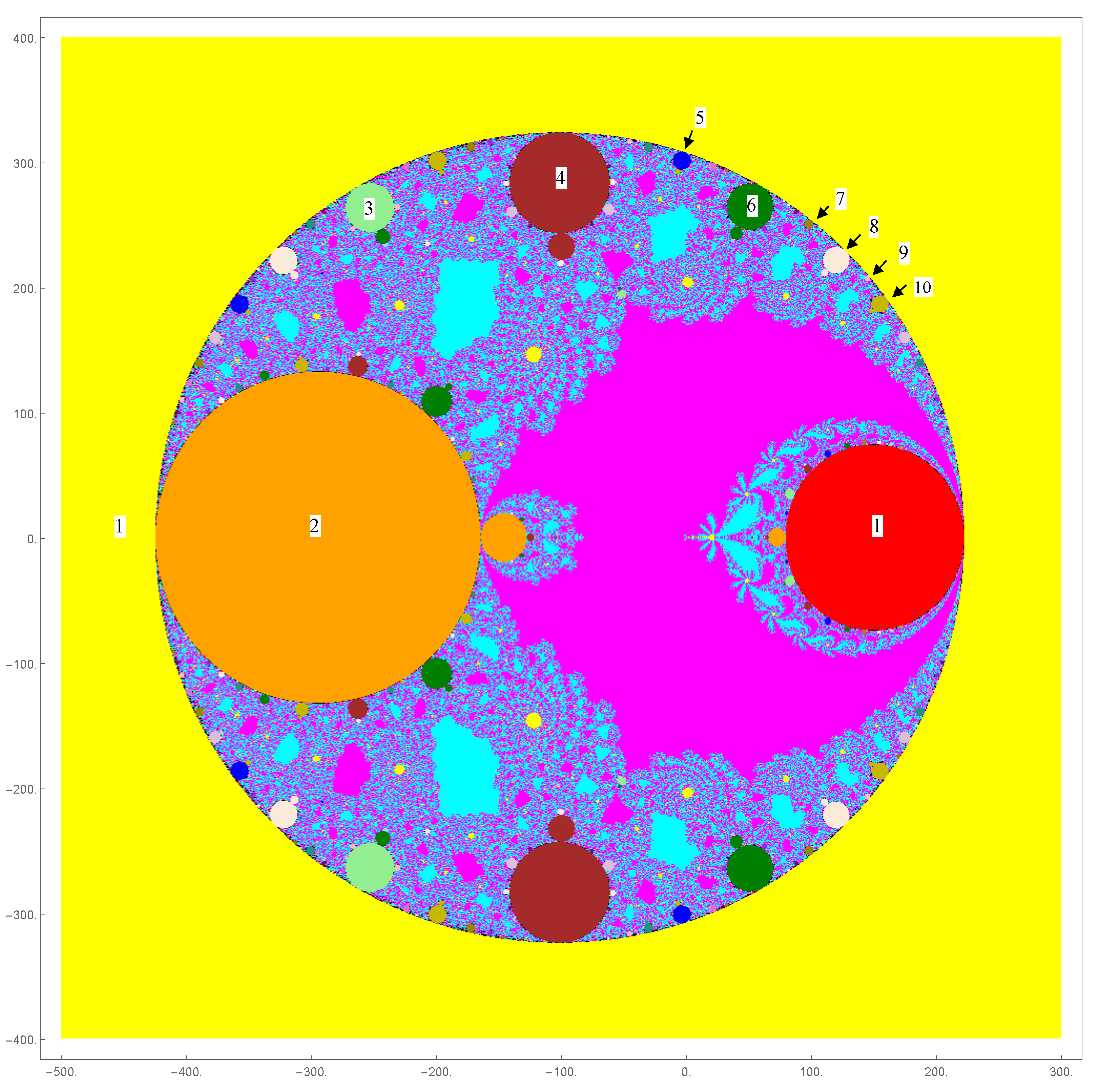
4.1. Parameter Space and Critical Orbit Behavior under the Conjugated Map $J(z;\lambda )$

We introduce the following notion of the parameter space $\mathcal{P}$ [13] to treat the underlying dynamics of J as $\lambda$ varies continuously on $\mathbb{C}$:

$$\begin{array}{c}\mathcal{P}=\{\lambda \in \mathbb{C}:\mathrm{an}\mathrm{orbit}\mathrm{of}\mathrm{a}\mathrm{critical}\mathrm{pointztends}\mathrm{to}\mathrm{a}\mathrm{number}\gamma \in \overline{\mathbb{C}}\mathrm{under}\mathrm{the}\mathrm{action}\mathrm{of}J(z;\lambda )\}.\hfill \end{array}$$

We will concentrate on the long-term behavior of the orbit of a $\lambda$-dependent critical point ${\zeta }_{\lambda }$ satisfying $Q({\zeta }_{\lambda };\lambda )=0$ under the action of the conjugated map $J({\zeta }_{\lambda };\lambda )$. Suppose that the long-term orbit of $J({\zeta }_{\lambda };\lambda )$ tends to a number $\gamma \in \overline{\mathbb{C}}$. Such $\gamma$ will be either ∞ or finite. Since ∞ is only a single point on $\overline{\mathbb{C}}$, it draws very little attention to the limit behavior. On the other hand, the finite $\gamma$ will cause the limit behavior to exhibit diverse patterns of convergence as $\lambda$ varies on $\mathbb{C}$.

To be more specific for the finite $\gamma$ with its boundedness, in view of Bolzano–Weierstass Theorem, there exists a convergent subsequence of the critical orbit under $J({\zeta }_{\lambda };\lambda )$. That is to say, there exists a q-periodic point $\xi \left(\lambda \right)$ for some $q\in \mathbb{N}$ such that

$$\xi \left(\lambda \right)=\underset{\ell \to \infty }{lim}{J}^{\ell }({\zeta }_{\lambda };\lambda )=\underset{j\to \infty }{lim}{J}^{pj+q}({\zeta }_{\lambda };\lambda )=J^q\circ (\underset{j\to \infty }{lim}{J}^{pj}({\zeta }_{\lambda };\lambda )=J^q(\xi \left(\lambda \right);\lambda ),$$

(15)

by expressing $\ell =pj+q$ for any $\ell ,p,j\in \mathbb{N}$ with $p<\ell$ and $q\in \{0,1,2,\cdots ,p-1\}$; note that $q=0$ implies the existence of a non-periodic bounded orbit. In view of the discussion in Section 3, we find the possible fixed points $\xi \left(\lambda \right)\in \{0,1,\infty ,{\xi }_{\lambda }^{\left(k\right)},1/{\xi }_{\lambda }^{\left(k\right)},(1\le k\le 3)\}$. If, for any given $q\in \mathbb{N}$, we let $G(z;\lambda )=J^q(z;\lambda )-z$, then $G(z;\lambda )$ defines a bivariate rational function of z and $\lambda$ on $\overline{\mathbb{C}}$. Hence, $G(z;\lambda )$ has a finite number of zeros $z=\xi \left(\lambda \right)$ being the fixed points of $J^q(z;\lambda )$ for any given $q\in \mathbb{N}$, which implies that there exists a $\lambda$ for any periodic-point in the critical orbit of $J(z;\lambda )$.

We now discuss the stability of the q-periodic point $\xi \left(\lambda \right)$. Let us consider the case when $q=1$ first. For the fixed points $\xi \left(\lambda \right)\in \{0,\infty \}$, we find $J(0;\lambda )=0$ and $J(\infty ;\lambda )=\infty$ and recognize that both fixed points 0 and ∞ are super-attractive. Regions of corresponding $\lambda$-values are respectively colored in cyan and magenta in the parameter space $\mathcal{P}$ shown in Figure 1. For the fixed point $\xi \left(\lambda \right)=1$, we have $J(1;\lambda )=1$ and $J^{\prime }(1;\lambda )<1$ for $\lambda \in \mathit{Y}$ in view of Theorem 1. The region Y is colored in yellow shown in Figure 1. For the $\lambda$-dependent fixed points $\xi \left(\lambda \right)\in \{{\xi }_{\lambda }^{\left(k\right)},1/{\xi }_{\lambda }^{\left(k\right)}$ and $(1\le k\le 3)\}$, we find $J({\xi }_{\lambda }^{\left(k\right)};\lambda )={\xi }_{\lambda }^{\left(k\right)}$ and $J(1/{\xi }_{\lambda }^{\left(k\right)};\lambda )=1/{\xi }_{\lambda }^{\left(k\right)}$ for $1\le k\le 3$. Regions of $\lambda$-values for these fixed points $\xi \left(\lambda \right)$ are colored in red, as indicated in Figure 1. Boundaries of such regions are expected to consist of six branches associated with ${\xi }_{\lambda }^{\left(k\right)},1/{\xi }_{\lambda }^{\left(k\right)}$ for $1\le k\le 3$. Next, we consider the case when $q\ge 2$. Observe that the attracting fixed point $\xi \left(\lambda \right)=1$ maintains its stability for $\lambda \in Y$. As $\lambda$ crosses the finite boundary of Y; i.e., the circle S, the fixed point $\xi \left(\lambda \right)$, loses its stability, but other attracting q-periodic points satisfying

$$J^q(\xi \left(\lambda \right);\lambda )=\xi \left(\lambda \right),|\frac{d}{dz}{J}^q(z;\lambda ){|}_{z=\xi \left(\lambda \right)}<1,\mathrm{for}q\ge 2$$

begin to emerge along the circle S. Regions of $\lambda$-values for these q-periodic points are painted according to the coloring scheme in Table 1 of [13]. The following corollary and proposition state useful properties of a q-periodic point of J.

Corollary 2.

If $z\in \overline{\mathbb{C}}$ is a q-periodic point of J, then $\frac{1}{z}$ is another.

Proof. 

In view of Proposition 2-(c) and fixed point invariance property [17] under conjugacy $h\left(z\right)=\frac{1}{z}$ for q-fold composition of J, we find that $J^q(\frac{1}{z};\lambda )=\frac{1}{J^q(z;\lambda )}=\frac{1}{z}$ for any given $\lambda \in \mathbb{C}$. □

According to Remark 4 of [13], the orbit behavior of only one branch ${\zeta }_1$ would suffice to explore the dynamics under J. Figure 1 displays a parameter space $\mathcal{P}$ associated with free critical points ${\zeta }_1\left(\lambda \right)$. If an orbit of $J({\zeta }_1;\lambda )$ attracts to a q-periodic point for a given $\lambda \in \mathcal{P}$, then $\lambda$ is colored with code $c_q$ defined by Table 1 of [13] and illustrated in Figure 3 of [13]. The computing error bound of ${10}^{-6}$ has been assigned with maximal 3000 iterations to obtain the convergence of a q-periodic orbit in $\mathcal{P}$.

Theorem 3 of [13] is useful to describe the property of symmetry on the parameter space $\mathcal{P}$. As we can see $\mathcal{P}$ in Figure 1, some of q-periodic components are indicated by arrow numbers. If $\lambda$ is chosen in such a q-periodic component, then the orbit of critical point ${\zeta }_{\lambda }$ is attracted to a q-periodic point of J. Recall that the fixed points of $J(z;\lambda )$ from (13) are $0,1,\infty$ and $\xi \left(\lambda \right)$ satisfying $T\left(\xi \right(\lambda );\lambda )=0$. Having found $\lambda$-dependent critical points ${\zeta }_{\lambda }$ from the roots of $Q(z;\lambda )=0$, we need attention to their orbit behavior as $\lambda \in \mathcal{P}$ varies.

4.2. Locating and Counting Bifurcation Points of Satellite Components’ Budding along S

The recent work of Geum-Kim [13] has shown an extensive study on locating and counting bifurcation points of satellite components’ budding along S associated with fixed point $\xi =1$. The current work will focus on the bifurcation of the satellite components born along the boundary of the red fixed components denoted by $\mathsf{\Omega }$, as shown in Figure 2, associated with the $\lambda$-dependent fixed points ${\xi }_{\lambda }^{\left(k\right)}$ and $1/{\xi }_{\lambda }^{\left(k\right)}$ for $1\le k\le 3$. According to the analysis described in Section 5.1.1 of Geum-Kim [13], we state the governing equation for the bifurcation of a q-periodic component ${\mathit{H}}_q$, identified by an arrow number q in Figure 2, budding from $\mathsf{\Omega }$ as follows: with $\xi \in \{{\xi }_{\lambda }^{\left(k\right)},1/{\xi }_{\lambda }^{\left(k\right)}:1\le k\le 3\}$ as a typical $\lambda$-dependent fixed point of $T(z;\lambda )$ described in Section 3.

$$\left\{\begin{array}{c}{J}_{\lambda }^q\left(\xi \right)=J_{\lambda }\left(\xi \right)=\xi ,\hfill \\ \frac{d}{dz}{J}_{\lambda }^q{\left(z\right)|}_{z=\xi }={\beta }^q=1,\hfill \end{array}\right.$$

(16)

where $J_{\lambda }\left(\xi \right)$ denotes $J(\xi ;\lambda )$ and $\beta =J_{\lambda }^{\prime }\left(\xi \right)$ is the derivative of $J(z;\lambda )$ evaluated at $z=\xi$. Given $q\in \mathbb{N}$, by solving ${\beta }^q=1$ for $\beta$, we have

$$J_{\lambda }^{\prime }\left(\xi \right)=\beta =e^{i2\pi \ell /q},$$

(17)

with $\ell \in \left\{0,1,2,\cdots ,q-1\right\}$ and $\gcd (\ell ,q)=1$ for $\ell \ne 0$. Solving for $\lambda$ from the first and last relations in (16), we can locate $\lambda ={\lambda }_{\ell ,q}$; that is, the so-called $\ell /q$-bifurcation point [13] of $\mathsf{\Omega }$. Besides, the nature of integers ℓ and q enables us to perceive the number of bifurcation points ${\lambda }_{\ell ,q}$ as the length $|{\mathcal{F}}_n|$ of the Farey [15] sequence ${\mathcal{F}}_n$ of order n. In view of Theorem 4 in [13], $|{\mathcal{F}}_n|$ is given by:

$$|{\mathcal{F}}_n|=1+\sum _{k=1}^n\varphi \left(k\right),$$

(18)

with $\varphi \left(k\right)$ as Euler’s totient function.

In view of Proposition 2-(a), we expect three red fixed components $\mathsf{\Omega }$, each boundary of which consists of two analytic branches forming a piecewise, smooth, closed curve. Details of such a boundary curve along with the location of bifurcation points will be discussed in the next section.

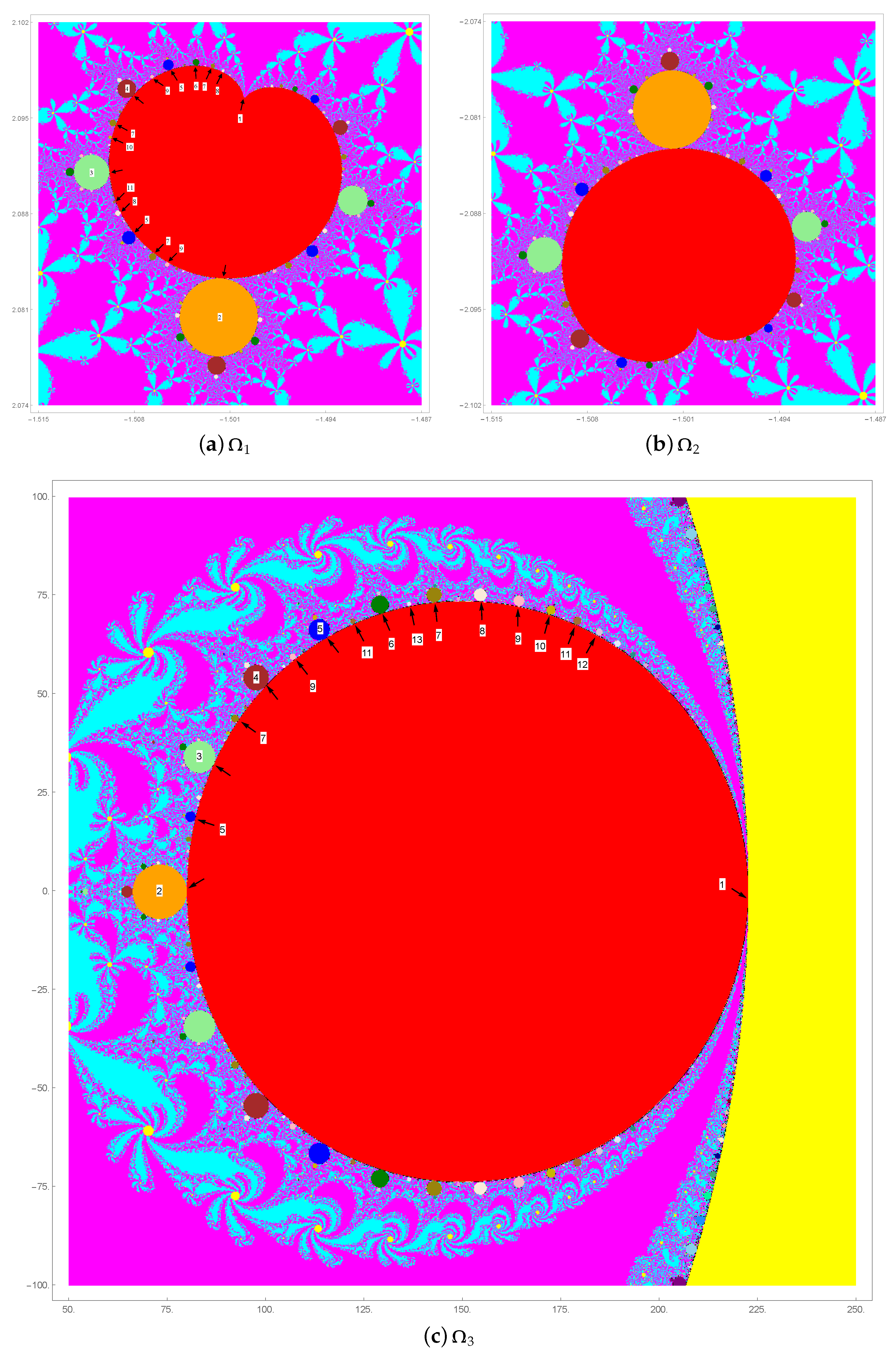
5. Boundary Curves of Red Fixed Components $\mathsf{\Omega }$

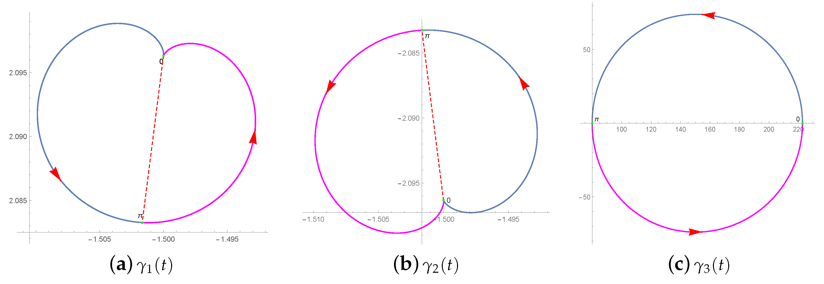
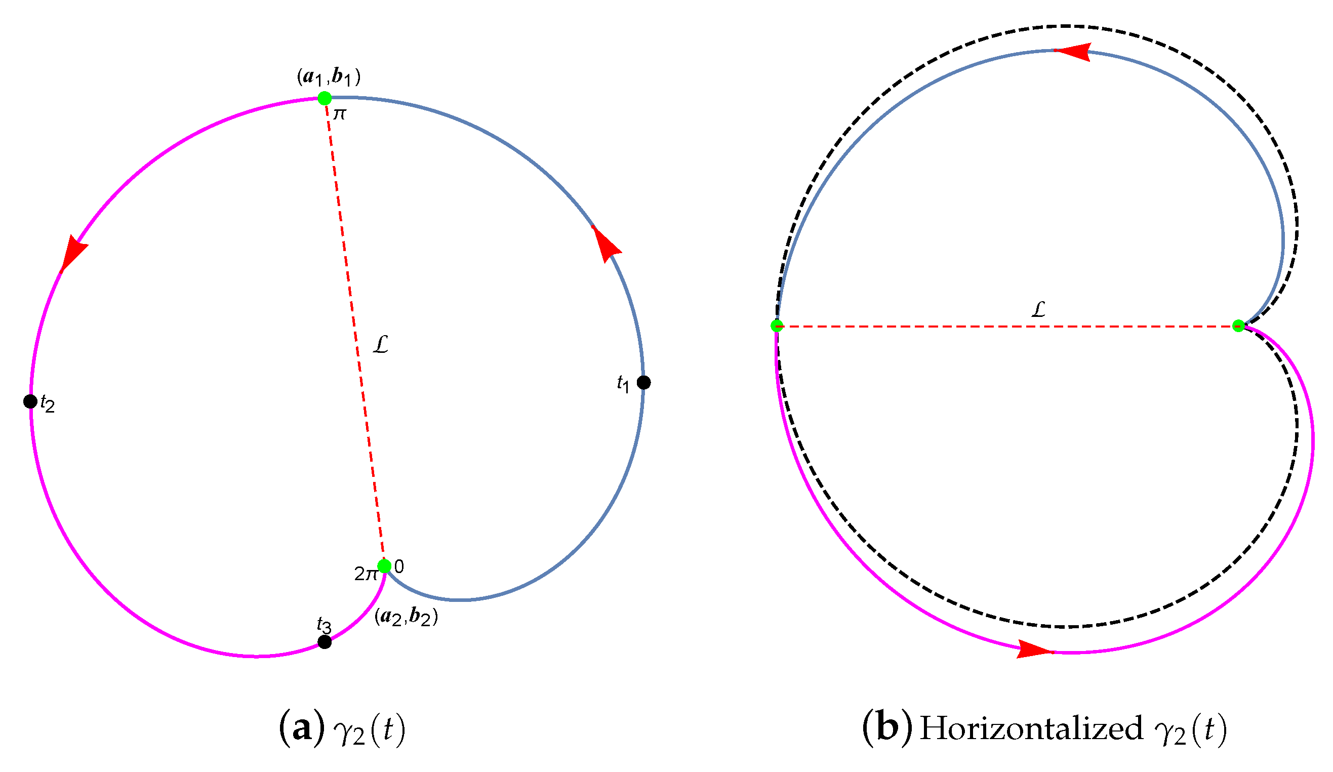
5.1. Parametric Boundary Equations of $\mathsf{\Omega }$

In this section, we seek a boundary equation for an attracting red fixed component $\mathsf{\Omega }$ associated with a typical $\lambda$-dependent fixed point $\xi$ given by a root of $T(z;\lambda )=0$. On the boundary, the fixed point $\xi$ will satisfy, in view of (12) and (13),

$$\left\{\begin{array}{cc}T(z;\lambda ){|}_{z=\xi }\hfill & {\displaystyle =81\prod _{k=1}^3(z^2+c_{k}z+1){|}_{z=\xi }=0,}\hfill \\ 324\left|\frac{z^3{(z+1)}^6{Q}_{\lambda }\left(z\right)}{q_{\lambda }{\left(z\right)}^2}\right|\hfill & =|J_{\lambda }^{\prime }\left(z\right){|}_{z=\xi }=1,\hfill \end{array}\right.$$

(19)

where $Q_{\lambda }\left(z\right),q_{\lambda }\left(z\right)$ and $J_{\lambda }\left(z\right)$, respectively, denote $Q(z;\lambda ),q(z;\lambda )$ and $J(z;\lambda )$ for convenience. Rewriting (19) with $i=\sqrt{-1}$ and t as a real parameter, we obtain

$${\displaystyle \prod _{k=1}^3(z^2+c_{k}z+1){|}_{z=\xi }=0\mathrm{and}\frac{324z^3{(z+1)}^6{Q}_{\lambda }\left(z\right)}{q_{\lambda }{\left(z\right)}^2}{|}_{z=\xi }=e^{it},0\le t\le 2\pi ,}$$

(20)

where $c_k$ are the three roots being dependent on $\lambda$ from Relation (14). To express $J_{\lambda }^{\prime }\left(\xi \right)$ in terms of $c_k$, we first let $\xi =z,c_k=c$ for brevity of notation, for the time being, and recall from (14) that

$$\lambda =\lambda \left(c\right)=-\frac{81}{32}(-16+18c-7c^2+c^3),$$

(21)

which comprises the boundary curves of $\mathsf{\Omega }$. Since three $\lambda$-values exist depending on $c_1,c_2,c_3$, we expect three red fixed components $\mathsf{\Omega }$. Now we write, with the help of Mathematica [20]:

$$\left\{\begin{array}{c}324z^3{(z+1)}^6{Q}_{\lambda }\left(z\right)=(z^2+cz+1)·{\mathsf{\Phi }}_q\left(z\right)+{\mathsf{\Phi }}_r\left(z\right),\hfill \\ q_{\lambda }{\left(z\right)}^2=(z^2+cz+1)·{\mathsf{\Psi }}_q\left(z\right)+{\mathsf{\Psi }}_r\left(z\right),\hfill \end{array}\right.$$

(22)

where ${\mathsf{\Phi }}_q\left(z\right)$ and ${\mathsf{\Psi }}_q\left(z\right)$ are polynomials of degree 9 and degree 6 in z, respectively; ${\mathsf{\Phi }}_r\left(z\right)=-13122{(c-2)}^4(14+c-7c^2+2c^3)\eta \left(z\right)$ and ${\mathsf{\Psi }}_r\left(z\right)=-6561{(c-2)}^7\eta \left(z\right)$ with $\eta \left(z\right)=c(c-1)(c+1)(c^2-3)+(c^3-c^2-2c+1)(c^3+c^2-2c-1)z$.

In view of the fact that $(z^2+cz+1)=0$ and the second relation of (20), we obtain

$$J_{\lambda }^{\prime }\left(\xi \right)=\frac{{\mathsf{\Phi }}_r\left(z\right)}{{\mathsf{\Psi }}_r\left(z\right)}{|}_{z=\xi }=\frac{2(2c^3-7c^2+c+14)}{{(c-2)}^3}=e^{it},0\le t\le 2\pi ,$$

(23)

where $c=c_k$ can be expressed in terms of $\lambda$ by the three roots of Relation (14) for any given $\lambda$. In fact, we are able to exactly find $c_k=c_k\left(t\right)$ for $1\le k\le 3$ and $0\le t\le 2\pi$ by solving the cubic equation given by the last relation of (23) as follows:

$$\left\{\begin{array}{c}{c}_1\left(t\right)=\frac{14-6e^{it}-2^{2/3}(9e^{it}-86)\sigma {\left(t\right)}^{-1/3}+2^{1/3}\sigma {\left(t\right)}^{1/3}}{3(4-e^{it})},\hfill \\ c_2\left(t\right)=\frac{14-6e^{it}+{(-1)}^{1/3}{2}^{2/3}(9e^{it}-86)\sigma {\left(t\right)}^{-1/3}+{(-1)}^{2/3}{2}^{1/3}\sigma {\left(t\right)}^{1/3}}{3(4-e^{it})},\hfill \\ c_3\left(t\right)=\frac{14-6e^{it}-{(-2)}^{2/3}(9e^{it}-86)\sigma {\left(t\right)}^{-1/3}-{(-2)}^{1/3}\sigma {\left(t\right)}^{1/3}}{3(4-e^{it})},\hfill \end{array}\right.$$

(24)

where $\sigma \left(t\right)=-1904+567e^{it}-54e^{2it}+3(e^{it}-4)\sqrt{16341-4050e^{it}+324e^{2it}}$.

Hence, using (24), we can express ${\lambda }_k=\lambda \left(c_k\left(t\right)\right)$ for $1\le k\le 3$ in (21) as a function of t and trace the boundaries of $\mathsf{\Omega }$ parametrically as $t\in [0,2\pi ]$ varies without difficulty. From an elementary theory of complex analysis, points at which a complex function $f\left(z\right)$ is not analytic on $\mathbb{C}$ are called singular points or singularities of $f\left(z\right)$. We remark that the unit circle $e^{it},t\in [0,2\pi )$ has singular points at $t=0$ and $t=\pi$. Therefore, $c_k\left(t\right)$ and $\lambda \left(c_k\left(t\right)\right)$ have also such singular points at $t=0$ and $t=\pi$.

We denote $F_k\left(t\right)=\lambda \left(c_k\left(t\right)\right)$ for $t\in [0,2\pi )$ for ease of continuing discussion of parametric curves. Due to the singularities, $F_k\left(t\right)$ consists of two piecewise analytic branches, one and the other of which trace along the curves for $t\in [0,\pi ]$ and $t\in (\pi ,2\pi )$, respectively. By means of elaborate computations, we find the following:

$$\left\{\begin{array}{ccc}\overline{c_1(\pi +t)}\hfill & =c_1(\pi -t),\hfill & \mathrm{for}t\in [0,\pi ],\hfill \\ \overline{c_3(\pi -t)}\hfill & =c_2(\pi +t),\hfill & \mathrm{for}t\in [0,\pi ],\hfill \\ \overline{c_2\left(t\right)}\hfill & =c_3(2\pi -t),\hfill & \mathrm{for}t\in [0,\pi ],\hfill \end{array}\right.$$

(25)

where $\overline{\beta }$ indicates the complex conjugate of $\beta$. Hence $F_k\left(t\right)=\lambda \left(c_k\left(t\right)\right)$ given by (21) satisfies the following relations among their six branches of $\mathsf{\Omega }$:

$$\left\{\begin{array}{ccc}\overline{F_1(\pi +t)}\hfill & =F_1(\pi -t),\hfill & \mathrm{for}t\in [0,\pi ],\hfill \\ \overline{F_3(\pi -t)}\hfill & =F_2(\pi +t),\hfill & \mathrm{for}t\in [0,\pi ],\hfill \\ \overline{F_2\left(t\right)}\hfill & =F_3(2\pi -t),\hfill & \mathrm{for}t\in [0,\pi ].\hfill \end{array}\right.$$

(26)

We further observe that the following relations hold at the singular points $t=0$ and $t=\pi$:

$$\left\{\begin{array}{ccc}{F}_3\left(0\right)=F_1\left(2{\pi }_{-}\right),\hfill & F_3\left(\pi \right)=F_1\left({\pi }_{+}\right),\hfill & F_1\left(0\right)=F_2\left(2{\pi }_{-}\right),\hfill \\ F_1\left(\pi \right)=F_2\left({\pi }_{+}\right),\hfill & F_2\left(0\right)=F_3\left(2{\pi }_{-}\right),\hfill & F_2\left(\pi \right)=F_3\left({\pi }_{+}\right),\hfill \end{array}\right.$$

(27)

where $a_{+}$ and $b_{-}$ indicate the approaches from the above of a and the below of b, respectively. This observation would suggest us to define three closed boundary curves ${\gamma }_j\left(t\right),(1\le j\le 3)$ of $\mathsf{\Omega }$:

$${\gamma }_1\left(t\right)=\left\{\begin{array}{c}{F}_3\left(t\right),t\in [0,\pi ],\hfill \\ F_1\left(t\right),t\in (\pi ,2\pi ),\hfill \end{array}\right.{\gamma }_2\left(t\right)=\left\{\begin{array}{c}{F}_1\left(t\right),t\in [0,\pi ],\hfill \\ F_2\left(t\right),t\in (\pi ,2\pi ),\hfill \end{array}\right.{\gamma }_3\left(t\right)=\left\{\begin{array}{c}{F}_2\left(t\right),t\in [0,\pi ],\hfill \\ F_3\left(t\right),t\in (\pi ,2\pi ),\hfill \end{array}\right.$$

(28)

each of which consists of two piecewise analytic arcs having singular branch points at $t=0$ and $t=\pi$. The boundary curves ${\gamma }_j\left(t\right),(1\le j\le 3)$ are parametrically plotted for $t\in [0,2\pi )$ in Figure 3. We will denote the red fixed component $\mathsf{\Omega }$ with boundary curve ${\gamma }_j\left(t\right)$ by ${\mathsf{\Omega }}_j$, as shown in Figure 2. The blue arcs are indeed the reflections of magenta arcs with respect to the real axis of the parameter space $\mathcal{P}$, which is expected in view of Theorem 3 of [13], and thus, yields the relation ${\gamma }_2\left(t\right)$ = $\overline{{\gamma }_1\left(t\right)}$.

Some Geometric Properties of Boundary Curves of $\mathsf{\Omega }$

We further investigate some geometric properties of ${\gamma }_j\left(t\right)$, including their arc lengths and bounding areas. Let $x_j\left(t\right)=\Re \left(F_j\left(t\right)\right)$ and $y_j\left(t\right)=\Im \left(F_j\left(t\right)\right)$. Then the arc lengths of ${\gamma }_j\left(t\right)$ are given by:

$$\begin{array}{c}{\displaystyle \widehat{|{\gamma }_1\left(t\right)|}={\int }_0^{\pi }\sqrt{x_3^{\prime }{\left(t\right)}^2+y_3^{\prime }{\left(t\right)}^2}dt+\underset{ϵ\to 0}{lim}{\int }_{\pi +ϵ}^{2\pi -ϵ}\sqrt{x_1^{\prime }{\left(t\right)}^2+y_1^{\prime }{\left(t\right)}^2}dt\approx 0.05285834292,}\hfill \\ \widehat{|{\gamma }_2\left(t\right)|}=\widehat{\left|{\gamma }_1\left(t\right)\right|},\mathrm{and}\widehat{\left|{\gamma }_3\left(t\right)\right|}=2{\int }_0^{\pi }\sqrt{x_2^{\prime }{\left(t\right)}^2+y_2^{\prime }{\left(t\right)}^2}dt\approx 457.0267546,\hfill \end{array}$$

(29)

with approximately 10 digits of accuracy.

Let ${\mathcal{A}}_j$ denote the area enclosed by ${\gamma }_j\left(t\right)$. Then, ${\mathcal{A}}_3=2{\int }_0^{\pi }{y}_2\left(t\right)x_2^{\prime }\left(t\right)dt\approx 16613.1610359$. It can be shown that $y_2\left(t\right)$ has a maximum $73.8923472569$ at $t=0.825122565614$ and a length $142.75$ of the diametral chord connecting two points at $t=0$ and $t=\pi$. Hence, ${\gamma }_3\left(t\right)$ is not a circle. To find ${\mathcal{A}}_2$, we consider Figure 4.

Let $(a_2,b_2)=(-1.4999999999999747,-2.096313728906051)$ and $(a_1,b_1)$ = (−1.501660908323884, −2.083261023446004) denote the points on ${\gamma }_2\left(t\right)$ at $t=0$ and $t=\pi$, respectively. Note that the diametral chord $\mathcal{L}$ connecting points $(a_2,b_2)$ and $(a_1,b_1)$ is parametrically represented by $\left(\frac{1}{\pi }(a_1-a_2)t+a_2,\frac{1}{\pi }(b_1-b_2)t+b_2\right)$ for $t\in [0,\pi ]$. Let $t_1$, $t_2$ and $t_3$ be, respectively, the points such that $x_1\left(t_1\right)$ is a maximum of $x_1\left(t\right)$, and $x_2\left(t_2\right)$ is a minimum of $x_2\left(t\right)$ and $x_2\left(t_3\right)=a_1$, along with computed values: $t_1=1.893100565129962$, $t_2=4.241197476773221$ and $t_3=5.478620432252566$. Let ${\mathcal{A}}_{2a}$ denote an area of the portion bounded by the blue arc and the diametral chord $\mathcal{L}$ and ${\mathcal{A}}_{2b}$ an area of the other remaining portion in Figure 4a. Then we find:

$\begin{array}{ll}{\mathcal{A}}_{2a}& ={\int }_{t_1}^{\pi }{y}_1\left(t\right)x_1^{\prime }\left(t\right)dt-{\int }_0^{t_1}{y}_1\left(t\right)x_1^{\prime }\left(t\right)dt-{\int }_0^{\pi }(\frac{1}{\pi }(b_1-b_2)t+b_2)\frac{1}{\pi }(a_1-a_2)dt\\ & \approx 0.00009026914890\end{array}$.

$\begin{array}{ll}{\mathcal{A}}_{2b}& ={\displaystyle \underset{ϵ\to 0}{lim}}\left({\int }_{\pi +ϵ}^{t_2}{y}_2\left(t\right)x_2^{\prime }\left(t\right)dt-{\int }_{t_2}^{2\pi -ϵ}{y}_2\left(t\right)x_2^{\prime }\left(t\right)dt+{\int }_0^{\pi }(\frac{1}{\pi }(b_1-b_2)t+b_2)\frac{1}{\pi }(a_1-a_2)dt\right)\\ & \approx 0.0001155066503\end{array}$.

Hence we have ${\mathcal{A}}_2={\mathcal{A}}_{2a}+{\mathcal{A}}_{2b}={\mathcal{A}}_1\approx 0.0002057757992$. We consider a translation and rotation of ${\gamma }_2\left(t\right)$ such that its diametral chord $\mathcal{L}$ lies along the horizontal axis and the point $(a_2,b_2)$ matches the origin, as shown in Figure 4b. Let ${\gamma }_c\left(t\right)$ be a boundary curve of a cardioid shown by a dotted line in Figure 4b and be parametrically represented by $x\left(t\right)=a(1-cost)cost$ and $y\left(t\right)=a(1-cost)sint$ for $t\in [0,2\pi ]$, with a as the half of the same length of $\mathcal{L}$. The length of ${\gamma }_c\left(t\right)$ and its bounding area are approximately given by $0.05263181338$ and $0.0002039660215$, respectively. Evidently, the red fixed component ${\mathsf{\Omega }}_2$ or ${\mathsf{\Omega }}_1$ is slightly larger than the cardioid with boundary curve ${\gamma }_c\left(t\right)$.

5.2. Location and Number of Bifurcation Points along the Boundaries of $\mathsf{\Omega }$

Table 1. Typical  $\ell /q$–bifurcation points ${\lambda }_{\ell ,q}$ for $1\le q\le 10$ along ${\gamma }_1\left(t\right)$.

q	ℓ
	0	1	2	3	4	5	6	7	8	9
1	${\left(\begin{array}{c}-1.5\\ 2.09631\end{array}\right)}^{*}$
2		$\left(\begin{array}{c}-1.50166\\ 2.08326\end{array}\right)$
3		$\left(\begin{array}{c}-1.50985\\ 2.09112\end{array}\right)$	$\left(\begin{array}{c}-1.49305\\ 2.08925\end{array}\right)$
4		$\left(\begin{array}{c}-1.50805\\ 2.09671\end{array}\right)$		$\left(\begin{array}{c}-1.49342\\ 2.09409\end{array}\right)$
5		$\left(\begin{array}{c}-1.50538\\ 2.09853\end{array}\right)$	$\left(\begin{array}{c}-1.50803\\ 2.08654\end{array}\right)$	$\left(\begin{array}{c}-1.49527\\ 2.08558\end{array}\right)$	$\left(\begin{array}{c}-1.49499\\ 2.09616\end{array}\right)$
6		$\left(\begin{array}{c}-1.50349\\ 2.09885\end{array}\right)$				$\left(\begin{array}{c}-1.49631\\ 2.09695\end{array}\right)$
7		$\left(\begin{array}{c}-1.5023\\ 2.09868\end{array}\right)$	$\left(\begin{array}{c}-1.50935\\ 2.09456\end{array}\right)$	$\left(\begin{array}{c}-1.50651\\ 2.08505\end{array}\right)$	$\left(\begin{array}{c}-1.49683\\ 2.08441\end{array}\right)$	$\left(\begin{array}{c}-1.49285\\ 2.09213\end{array}\right)$	$\left(\begin{array}{c}-1.49726\\ 2.09723\end{array}\right)$
8		$\left(\begin{array}{c}-1.50154\\ 2.09838\end{array}\right)$		$\left(\begin{array}{c}-1.50903\\ 2.08813\end{array}\right)$		$\left(\begin{array}{c}-1.49419\\ 2.08684\end{array}\right)$		$\left(\begin{array}{c}-1.49793\\ 2.09728\end{array}\right)$
9		$\left(\begin{array}{c}-1.50106\\ 2.09809\end{array}\right)$	$\left(\begin{array}{c}-1.50664\\ 2.09792\end{array}\right)$		$\left(\begin{array}{c}-1.50553\\ 2.0844\end{array}\right)$	$\left(\begin{array}{c}-1.49781\\ 2.08392\end{array}\right)$		$\left(\begin{array}{c}-1.4942\\ 2.09536\end{array}\right)$	$\left(\begin{array}{c}-1.4984\\ 2.09724\end{array}\right)$
10		$\left(\begin{array}{c}-1.50075\\ 2.09783\end{array}\right)$		$\left(\begin{array}{c}-1.50966\\ 2.09357\end{array}\right)$				$\left(\begin{array}{c}-1.49279\\ 2.09128\end{array}\right)$		$\left(\begin{array}{c}-1.49874\\ 2.09718\end{array}\right)$

${}^{*}$—$\left(\begin{array}{c}-1.5\\ 2.09631\end{array}\right)\equiv -1.5+2.09631i,i=\sqrt{-1}$.

and

Table 2. Typical  $\ell /q$–bifurcation points ${\lambda }_{\ell ,q}$ for $1\le q\le 10$ along ${\gamma }_3\left(t\right)$.

q	ℓ
	0	1	2	3	4	5	6	7	8	9
1	222.75
2		79.9533
3		$\left(\begin{array}{c}86.8564\\ 32.5726\end{array}\right)$	$\left(\begin{array}{c}86.8564\\ -32.5726\end{array}\right)$
4		$\left(\begin{array}{c}99.9319\\ 52.1701\end{array}\right)$		$\left(\begin{array}{c}99.9319\\ -52.1701\end{array}\right)$
5		$\left(\begin{array}{c}114.967\\ 64.2308\end{array}\right)$	$\left(\begin{array}{c}82.1455\\ 18.7639\end{array}\right)$	$\left(\begin{array}{c}82.1455\\ -18.7639\end{array}\right)$	$\left(\begin{array}{c}114.967\\ -64.2308\end{array}\right)$
6		$\left(\begin{array}{c}129.717\\ 70.7847\end{array}\right)$				$\left(\begin{array}{c}129.717\\ -70.7847\end{array}\right)$
7		$\left(\begin{array}{c}143.019\\ 73.5133\end{array}\right)$	$\left(\begin{array}{c}92.962\\ 43.4756\end{array}\right)$	$\left(\begin{array}{c}81.0346\\ 13.2477\end{array}\right)$	$\left(\begin{array}{c}81.0346\\ -13.2477\end{array}\right)$	$\left(\begin{array}{c}92.962\\ -43.4756\end{array}\right)$	$\left(\begin{array}{c}143.019\\ -73.5133\end{array}\right)$
8		$\left(\begin{array}{c}154.482\\ 73.7669\end{array}\right)$		$\left(\begin{array}{c}83.5158\\ 23.7661\end{array}\right)$		$\left(\begin{array}{c}83.5158\\ -23.7661\end{array}\right)$		$\left(\begin{array}{c}154.482\\ -73.7669\end{array}\right)$
9		$\left(\begin{array}{c}164.133\\ 72.5165\end{array}\right)$	$\left(\begin{array}{c}107.372\\ 59.0033\end{array}\right)$		$\left(\begin{array}{c}80.5984\\ 10.2542\end{array}\right)$	$\left(\begin{array}{c}80.5984\\ -10.2542\end{array}\right)$		$\left(\begin{array}{c}107.372\\ -59.0033\end{array}\right)$	$\left(\begin{array}{c}164.133\\ -72.5165\end{array}\right)$
10		$\left(\begin{array}{c}172.175\\ 70.4101\end{array}\right)$		$\left(\begin{array}{c}90.8087\\ 40.1095\end{array}\right)$				$\left(\begin{array}{c}90.8087\\ -40.1095\end{array}\right)$		$\left(\begin{array}{c}172.175\\ -70.4101\end{array}\right)$

list typical values of ${\lambda }_{\ell ,q}$ for $1\le q\le 10$ on ${\gamma }_1\left(t\right)$ and ${\gamma }_3\left(t\right)$, respectively. In the sense of bifurcations discussed in [18], $\ell /q$–bifurcation points are types of flip, fold and Neimark–Sacker, respectively, when $q=1,q=2$ and $q\ge 3$. It is remarkable to note that the largest ${\mathit{H}}_q$ for $q\in \mathbb{N}$ are born at the desired bifurcation points in the order of Farey sequence along the upper branch of ${\gamma }_3\left(t\right)$ and along the left branch of ${\gamma }_1\left(t\right)$ or along the right branch of ${\gamma }_2\left(t\right)$. The $0/1$-bifurcation point is the one where the red fixed component $\mathsf{\Omega }$ is budded from itself or from other fixed component; its location was found to be $-1.5+2.09631i$ for ${\gamma }_1\left(t\right)$, and $222.75$ for ${\gamma }_3\left(t\right)$. These locations are, respectively, regarded as a bifurcation point for a red fixed primitive component, and as a bifurcation point for a red fixed satellite component budded from a yellow fixed component Y.

The number of bifurcation points is determined by the length of the Farey sequence mentioned in (18) of the preceding section.

6. Conclusions

We have analyzed the boundary curves of red fixed components $\mathsf{\Omega }$ in the parameter space for uniparametric Jarratt-type simple-root finders (1) with $H\left(t\right)$ in (2), under the Möbius conjugacy map applied to a simple quadratic polynomial. Extensive investigation has been done on the parametric the boundary equations of $\mathsf{\Omega }$ to explore bifurcation phenomena underlying the limit behavior of the iteration dynamics under conjugated map $J(z;\lambda )$. The desired bifurcation points have been successfully found and some of them are listed in Table 1 and Table 2. Despite that the boundary curves of ${\mathsf{\Omega }}_2$ and ${\mathsf{\Omega }}_3$, respectively, appear to be a cardioid and a circle, they were found to be merely the cardioid-like and circle-like curves. It is interesting that the Farey sequence gives theoretical backgrounds on the number of bifurcation points and the manner of positioning of satellite components’ budding along the boundary curves.

Our next study primarily aims to analyze the boundary curves of higher-periodic components and to explore the bifurcation phenomena occurring along the boundary curves.

References

1. Behl, R.; Cordero, A.; Motsa, S.; Torregrosa, J. On developing fourth-order optimal families of methods for multiple roots and their dynamics. Appl. Math. Comput. 2015, 265, 520–532. [Google Scholar] [CrossRef] [Green Version]
2. Behl, R.; Cordero, A.; Motsa, S.; Torregrosa, J. Multiplicity anomalies of an optimal fourth-order class of iterative methods for solving nonlinear equations. Nonlinear Dyn. 2018, 91, 98–112. [Google Scholar] [CrossRef] [Green Version]
3. Geum, Y.H.; Kim, Y.I. A two-parameter family of fourth-order iterative methods with optimal convergence for multiple zeros. J. Appl. Math. 2013, 2013, 369067. [Google Scholar]
4. Geum, Y.H.; Kim, Y.I.; Magreñán, Á.A. A biparametric extension of King’s fourth-order methods and their dynamics. Appl. Math. Comput. 2016, 282, 254–275. [Google Scholar] [CrossRef]
5. Geum, Y.H.; Kim, Y.I.; Magreñán, Á.A. A study of dynamics via Mobius conjugacy map on a family of sixth-order modified Newton-like multiple-zero finders with bivariate polynomial weight functions. J. Comput. Appl. Math. 2018, 344, 608–623. [Google Scholar] [CrossRef]
6. Magreñán, Á.A. Different anomalies in a Jarratt family of iterative root-finding methods. Appl. Math. Comput. 2014, 233, 29–38. [Google Scholar]
7. Neta, B.; Scott, M.; Chun, C. Basin attractors for various methods for multiple roots. Appl. Math. Comput. 2012, 218, 5043–5066. [Google Scholar] [CrossRef]
8. García-Olívo, M.; Gutíerrez, J.M.; Magreñán, Á.A. A complex dynamical approach of Chebyshev’s method. SeMA J. 2015, 71, 57–68. [Google Scholar] [CrossRef]
9. Cordero, A.; Guasp, L.; Torregrosa, J.R. Fixed Point Root-Finding Methods of Fourth-Order of Convergence. Symmetry 2019, 11, 769. [Google Scholar] [CrossRef] [Green Version]
10. Ahlfors, L.V. Complex Analysis; McGraw-Hill Book, Inc.: New York, NY, USA, 1979. [Google Scholar]
11. Shabat, B.V. Introduction to Complex Analysis PART II, Functions of Several Variables; American Mathematical Society: Providence, RI, USA, 1992. [Google Scholar]
12. Blanchard, P. The dynamics of Newton’s method. In Proceedings of the Symposia in Applied Mathematics; American Mathematical Society: Providence, RI, USA, 1994; Volume 49, pp. 139–154. [Google Scholar]
13. Geum, Y.H.; Kim, Y.I. On Locating and Counting Satellite Components Born along the Stability Circle in the Parameter Space for a Family of Jarratt-Like Iterative Methods. Mathematics 2019, 7, 839. [Google Scholar] [CrossRef] [Green Version]
14. Peitgen, H.; Richter, P. The Beauty of Fractals; Springer: New York, NY, USA, 1986. [Google Scholar]
15. Ainsworth, J.; Dawson, M.; Pianta, J.; Warwick, J. The Farey Sequence. 2012. Available online: http://www.maths.ed.ac.uk/~aar/fareyproject.pdf (accessed on 2 April 2019).
16. Beardon, A.F. Iteration of Rational Functions; Springer: New York, NY, USA, 1991. [Google Scholar]
17. Lee, M.Y.; Kim, Y.I. The dynamical analysis of a uniparametric family of three-point optimal eighth-order multiple-root finders under the Möbius conjugacy map on the Riemann sphere. Numer. Algorithms 2019, 1–28. [Google Scholar] [CrossRef]
18. Nayfeh, A.H.; Balachandran, B. Applied Nonlinear Dynamics: Analytical, Computational, and Experimental Methods; John Wiley & Sons: New York, NY, USA, 2008. [Google Scholar]
19. Campos, B.; Cordero, A.; Torregrosa, J.R.; Vindel, P. Orbits of period two in the family of a multipoint variant of Chebyshev-Halley family. Numer. Algorithms 2016, 73, 141–156. [Google Scholar] [CrossRef] [Green Version]
20. Wolfram, S. The Mathematica Book, 5th ed.; Wolfram Media: Champaign, IL, USA, 2003. [Google Scholar]
Figure 1. Parameter space P associated with critical point ζ 1 ( λ ) .
Mathematics 08 00051 g001
Figure 2. The three red fixed components Ω .
Mathematics 08 00051 g002
Figure 3. Boundary curves of the three red fixed components Ω .
Mathematics 08 00051 g003
Figure 4. γ 2 ( t ) and the horizontalized γ 2 ( t ) .
Mathematics 08 00051 g004