Resources Planning for Container Terminal in a Maritime Supply Chain Using Multiple Particle Swarms Optimization (MPSO)


Abstract
1. Introduction
2. Literature Review
2.1. The Classification of Berth Allocation Problem (BAP) and Quay Crane Assignment Problem (QCAP)
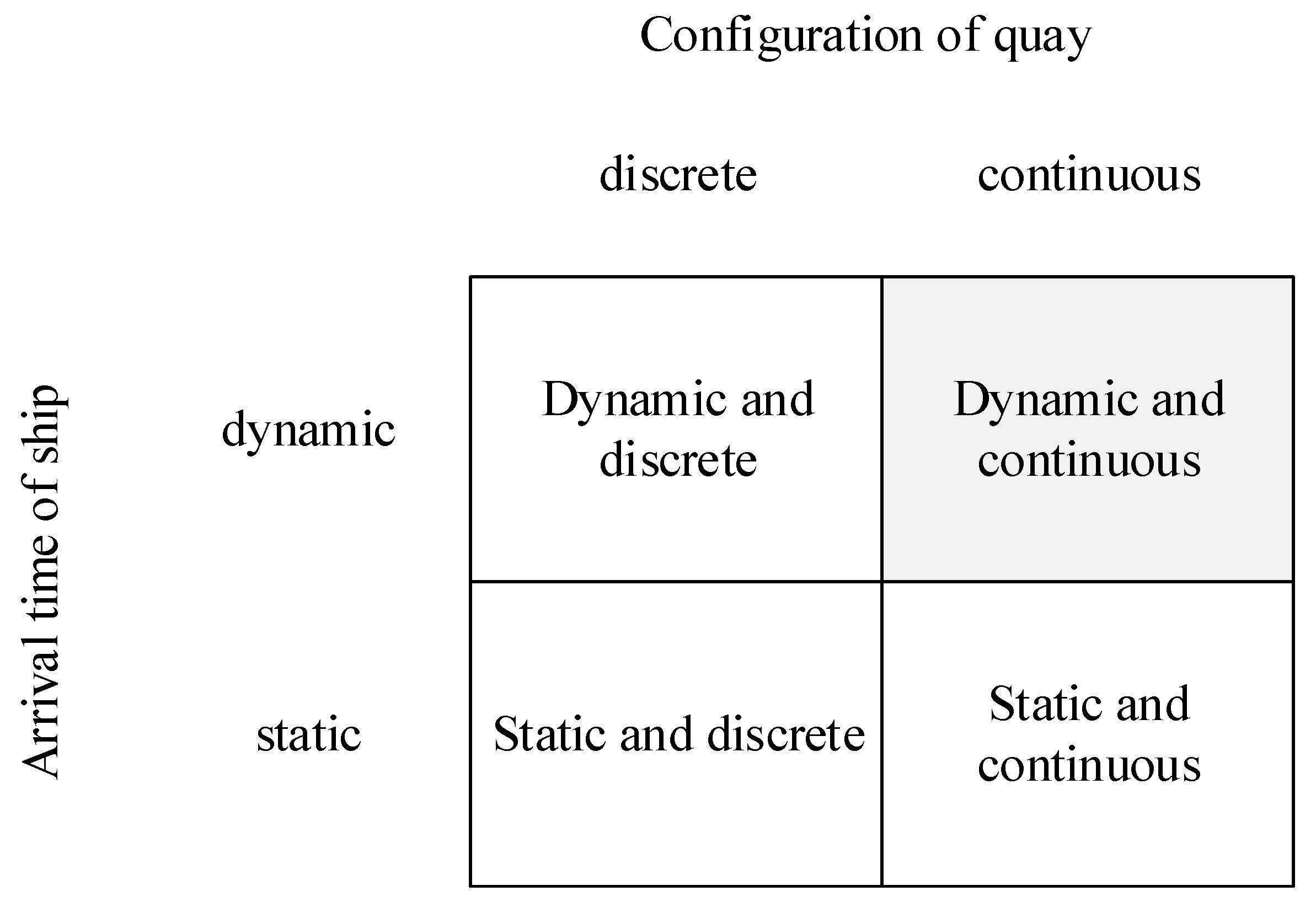
2.1.1. BAP Classification
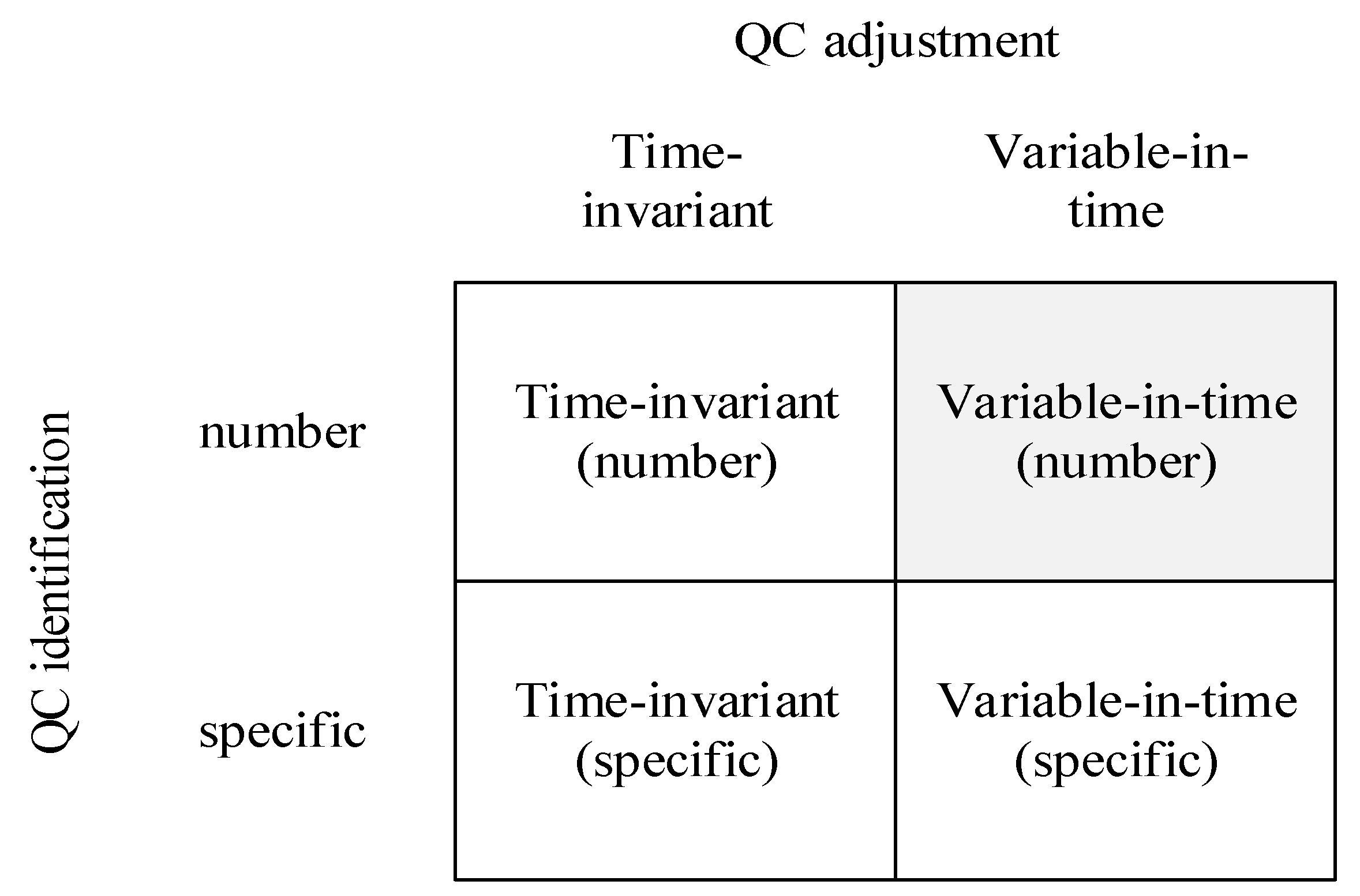
2.1.2. QCAP Classification
2.2. Relevant Studies
3. Formulation of a Mathematical Model for Simultaneous DCBAP and QCAP
3.1. Problem Definition
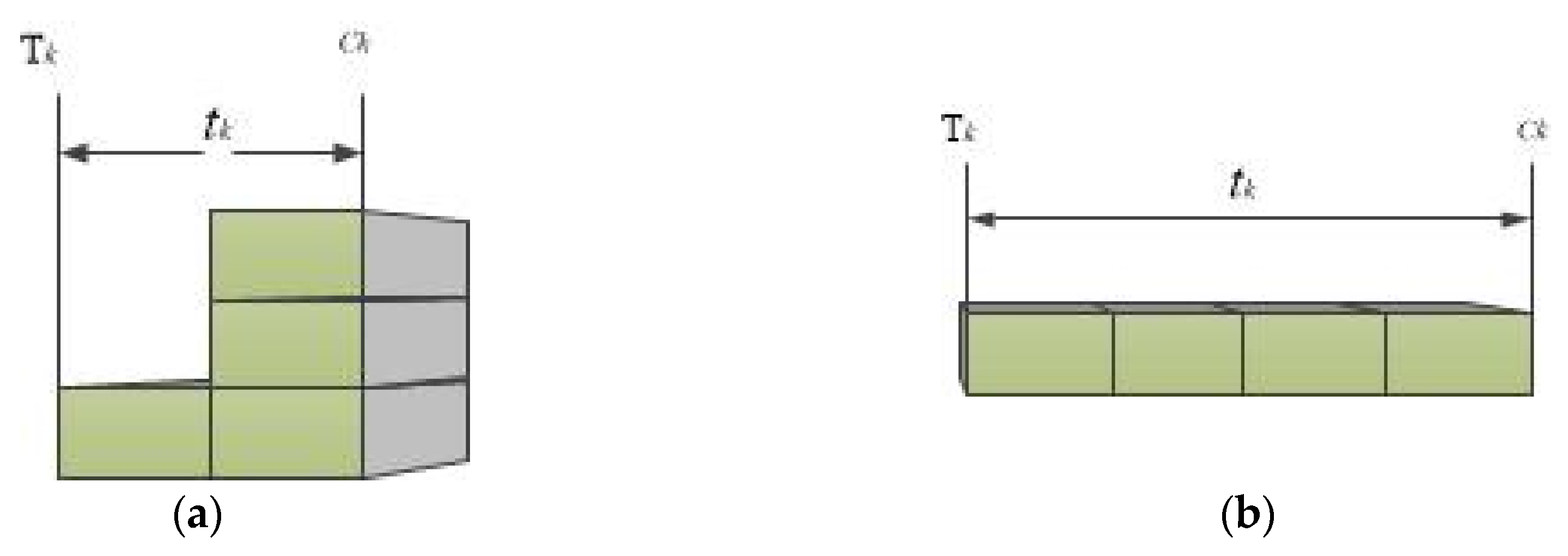
3.2. The Estimation of Handling Time for a Ship
| the QC capacity required for the ship k | |
| the maximum number of QCs assignable to ship k | |
| the berth deviation of a ship k from its desired berthing position | |
| the berth deviation factor | |
| the interference exponent of QCs |
- is the actual berthing position of ship k
- is the desired berthing position of the ship k
| the total number of containers to be handled for the ship k | |
| the number of QCs assigned to the ship k | |
| the berth deviation | |
| the berth deviation factor |
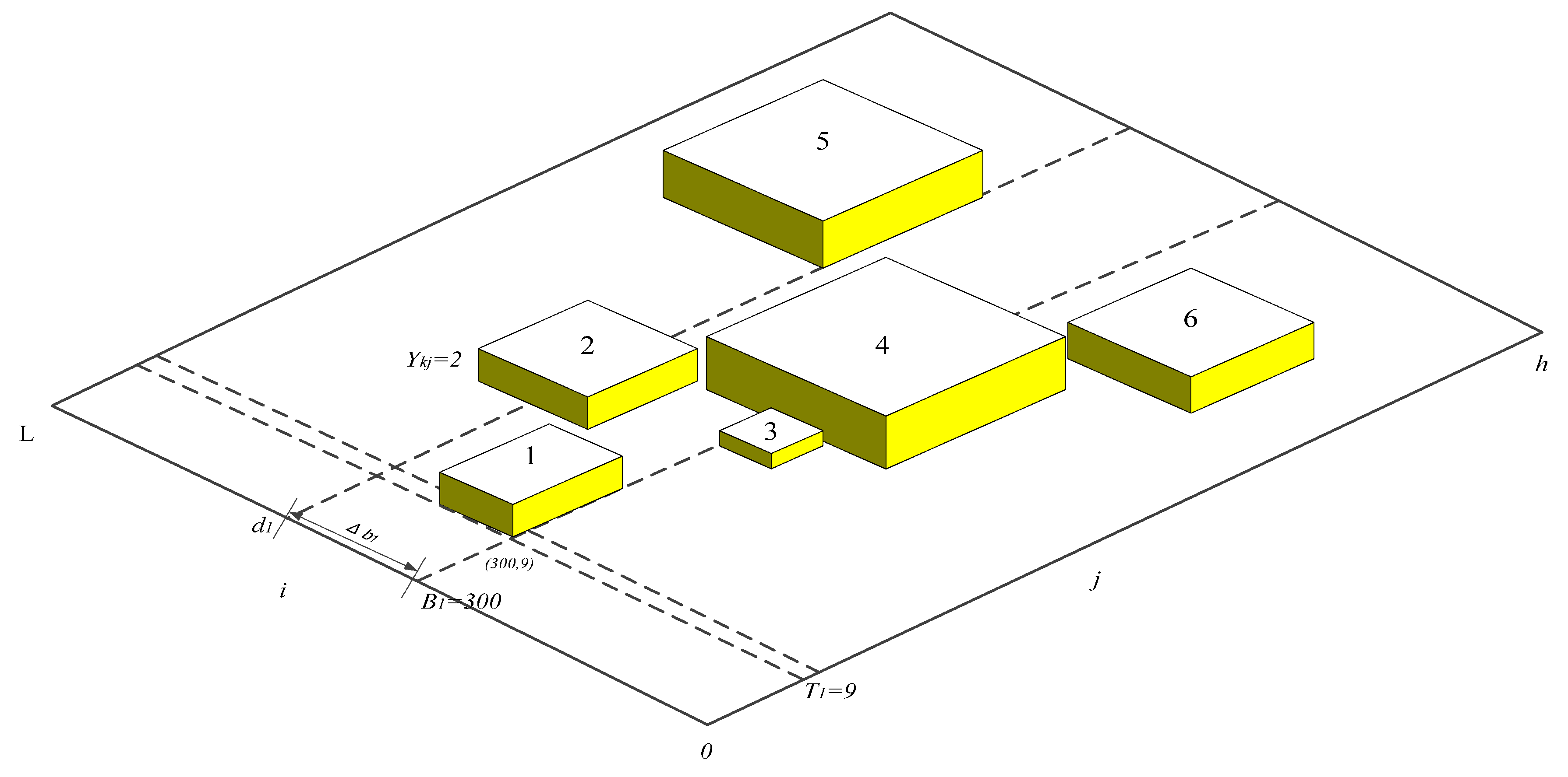
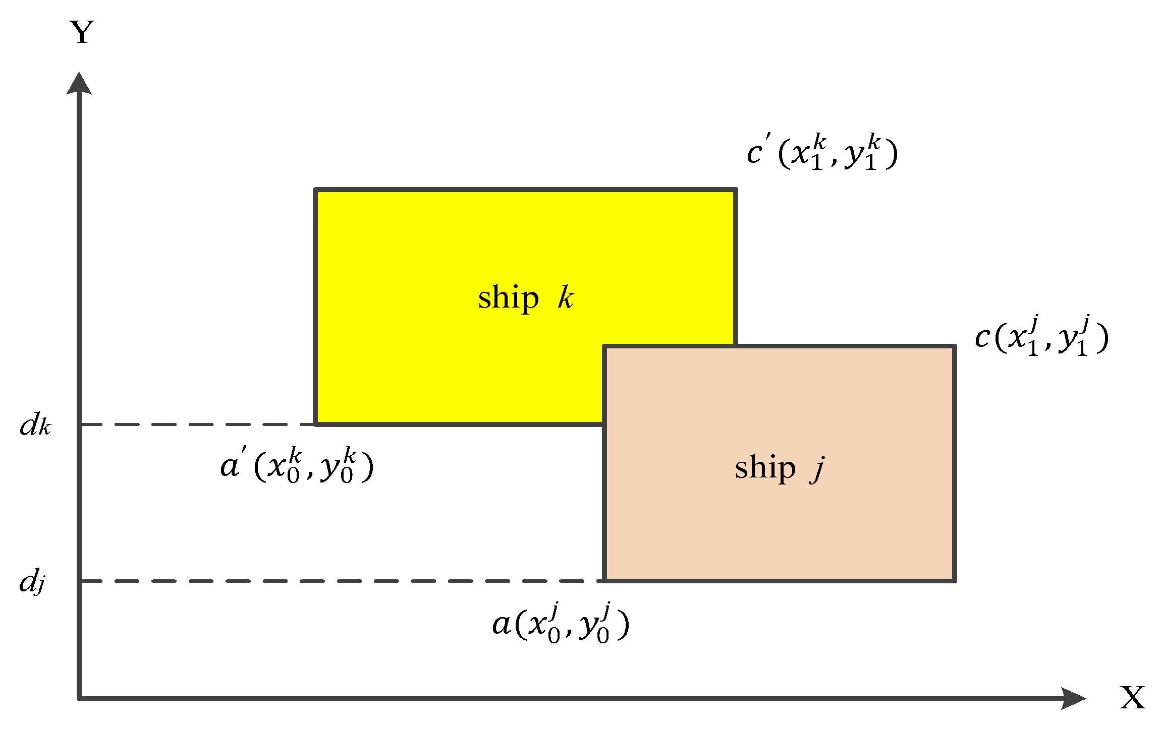
3.3. Berthing Plan
3.4. Mathematical Model
- Each ship is handled continuously until it is completed.
- Inter-ship clearance distance is included in ship length.
- A ship departs immediately when handling completed.
| i | a berth position; i . |
| j | a time segment; j . |
| k | a ship number; k . |
| q, | QC number; q, . |
| L H T N Q C1 C2 | the quay length (meters) the total number of segments (each is one hour) within the planning horizon the set of time periods, T = {1,…,H} the total number of calling ships within the planning horizon the total number of QCs the length of ship k the minimum number of QC assignable to ship k the maximum number of QC assignable to ship k the expected arrival time of ship k the total number of loading and unloading containers for ship k at this port the desired berthing position of ship k the interference exponent of QCs (0 the berth deviation factor; the increase rate of QC capacity/one berth deviation ( the cost rate of handling time (Twenty foot equivalent units (TEUs)/hour) the cost rate of waiting time |
| the number of QCs assigned to ship k at the time period j | |
| the berthing position of ship k ( | |
| the beginning berthing time of ship k ( |
4. Multiple Particle Swarm Optimization (MPSO)
4.1. PSO
4.2. The MPSO
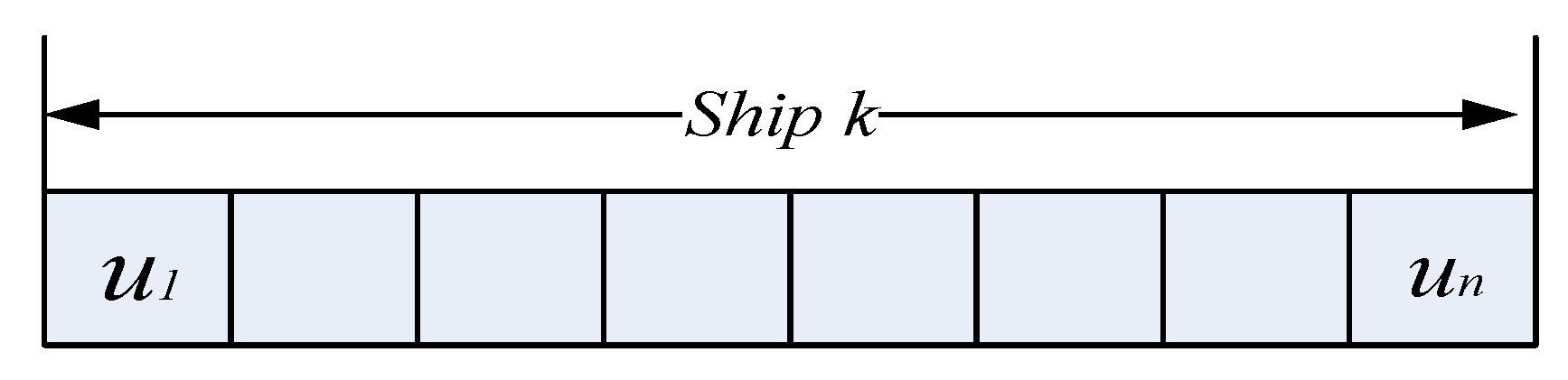
4.2.1. Position Representation for a Particle
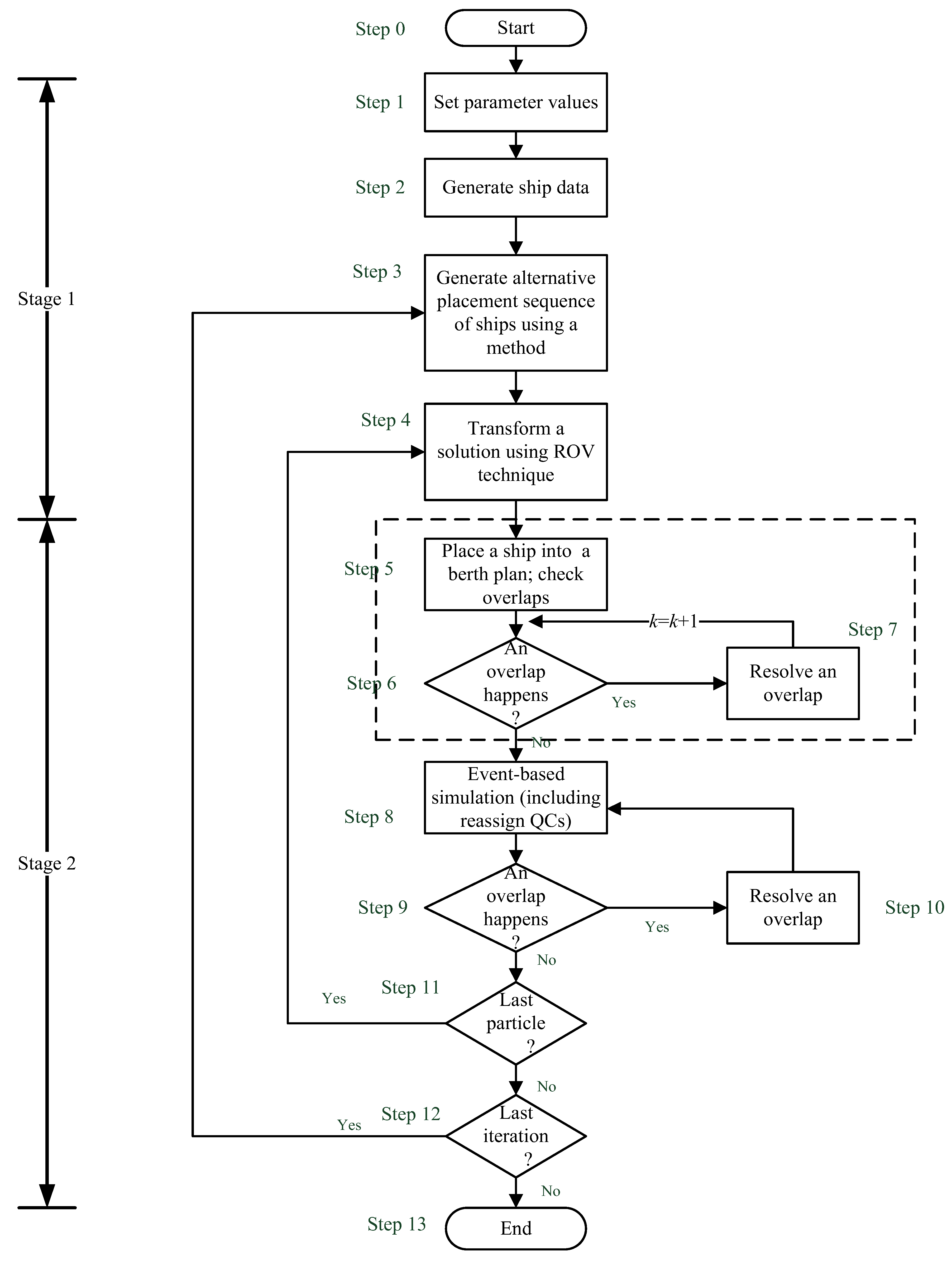
4.2.2. The Two-Stage Procedure
4.2.3. Details of the Main Tasks in the Second Stage
| the number of QCs assigned to ship k at the stage ; | |
| the number of QCs assigned to ship k at the stage ; |
4.2.4. The Features of the MPSO
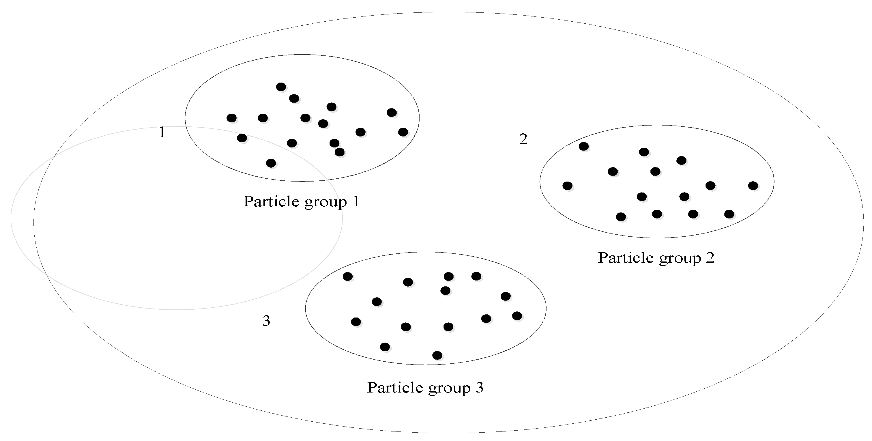
Multiple Groups of Particles
Regrouping Mechanism
Self-Adaptive Velocity
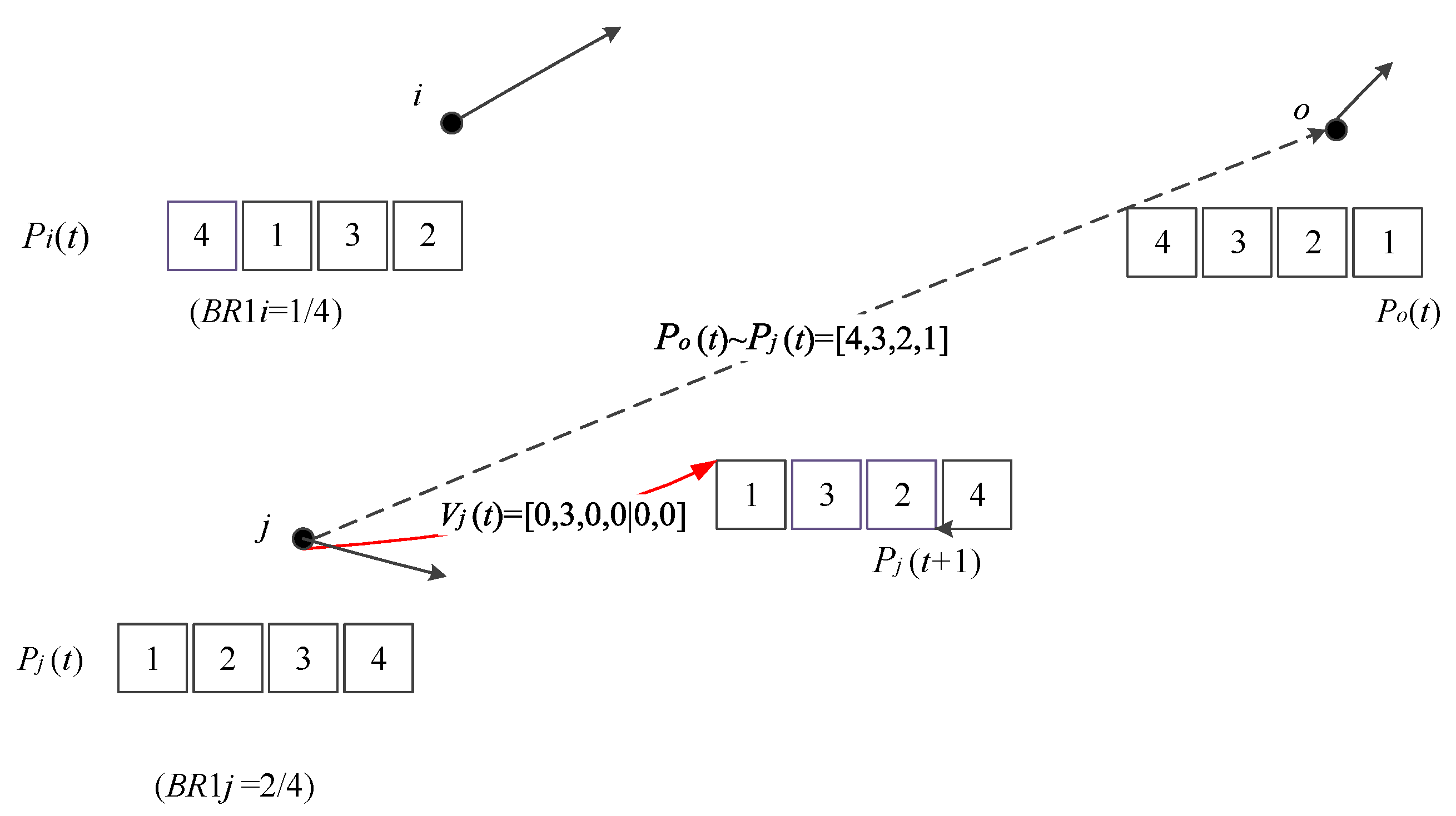
Intelligent Movement of a Particle
- Direct-fly prevention: the direct-fly prevention is a mechanism stopping a particle from flying to the target particle in the next step because such a move will waste one local search. Specifically, the MPSO will measure the current distance between a particle j and a target particle o. If the distance between them is satisfied with the condition, , the MPSO then stops generating binary value 1 for the of the particle j as additional one binary value 1 added to the will trigger a direct-fly.
- Neighborhood search: while imposed by the direct-fly prevention, a particle will stay at its current position, which will waste one local search. For improvement, the function, exchange (p1,p2), is used for neighborhood search by exchanging two randomly-selected position elements in the position vector of a particle.
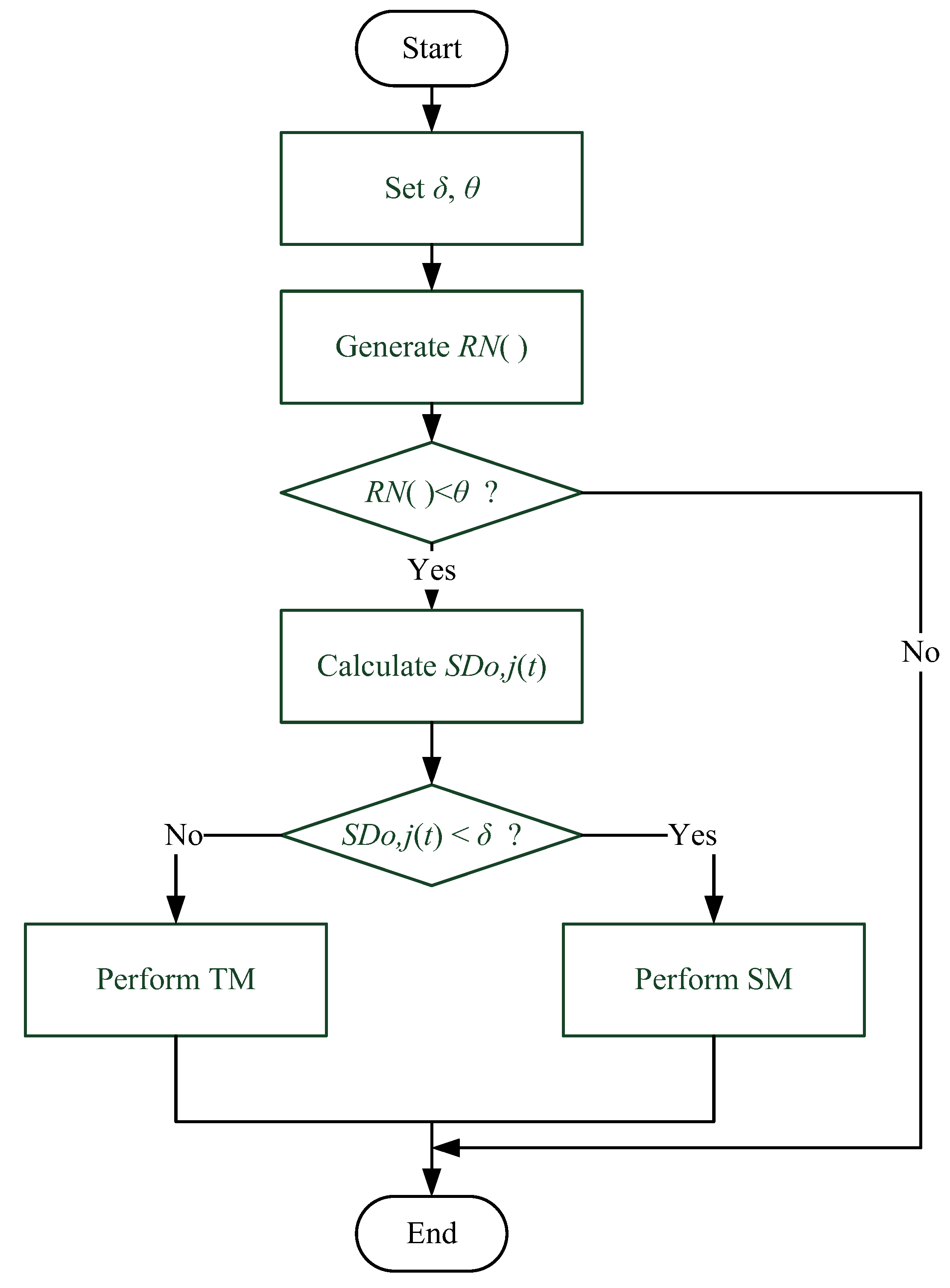
The Self-Adaptive Variant of a Particle
- Swap Mutation (SM): in this mutation two values of two positions (p1 < p2) are first randomly selected and then swapped.
- Thoros Mutation (TM): in this mutation three values of three positions p1, p2, and p3 (where p1 < p2 < p3) are first selected randomly, and then the value of p1 becomes the value of p2, the original value of p2 becomes the value of p3, and the original value of p3 becomes the value of p1. Compared with the SM, the TM has a greater variant due to more mutated values.
4.3. The Main Flow Logic of MPSO
| Algorithm 1. The logic flow of MPSO. | |
| 1 | Set parameter values (N, Rm, P, m, iterations, l_iter, etc.) |
| 2 | Initial positions for particles using rank order values (ROVs) |
| 3 | FOR (int t = 1; t <= iterations; t++){ |
| 4 | Calculate the Z values for all particles using Equation (6). |
| 5 | Rank particles according to their FVs |
| 6 | Generate groups m(t) for particles. |
| 7 | FOR (int li = 1;li< = l_iter; li++) |
| 8 | FOR (int j = 1; j <= m(t); j++) |
| 9 | FOR (int k = 1;k <= the_number_of_particles_in_j; k++) |
| 10 | IF particle k is not the best particle in the subgroup j |
| 11 | Move the particle k one step toward the best particle in j |
| 12 | Calculate Z value using Equation (6). |
| 13 | IF Z value of this movement is improved |
| 14 | Store the Z value for this particle k |
| 15 | Store the current position for this particle k |
| 16 | ELSE |
| 17 | Move the particle k toward the global best particle in the swarm |
| 18 | Calculate Z value using Equation (6). |
| 19 | IF Z value of this movement is improved |
| 20 | Store the Z value for this particle k |
| 21 | Store the current position for this particle k |
| 22 | ELSE |
| 23 | Change the particle k to a random position |
| 24 | END IF |
| 25 | END IF |
| 26 | Compare the solution to the global best solution |
| 27 | IF better |
| 28 | Store the solution as the global best solution |
| 29 | END IF |
| 30 | Perform the self-adaptive variant for the particle k |
| 31 | END IF |
| 32 | END FOR k |
| 33 | END FOR j |
| 34 | END FOR li |
| 35 | END FORt |
5. Numerical Example
5.1. Parameters Setting for Experiments
5.2. A Small-Size Example
5.3. Experiments
5.4. Analysis and Discussion
- (1)
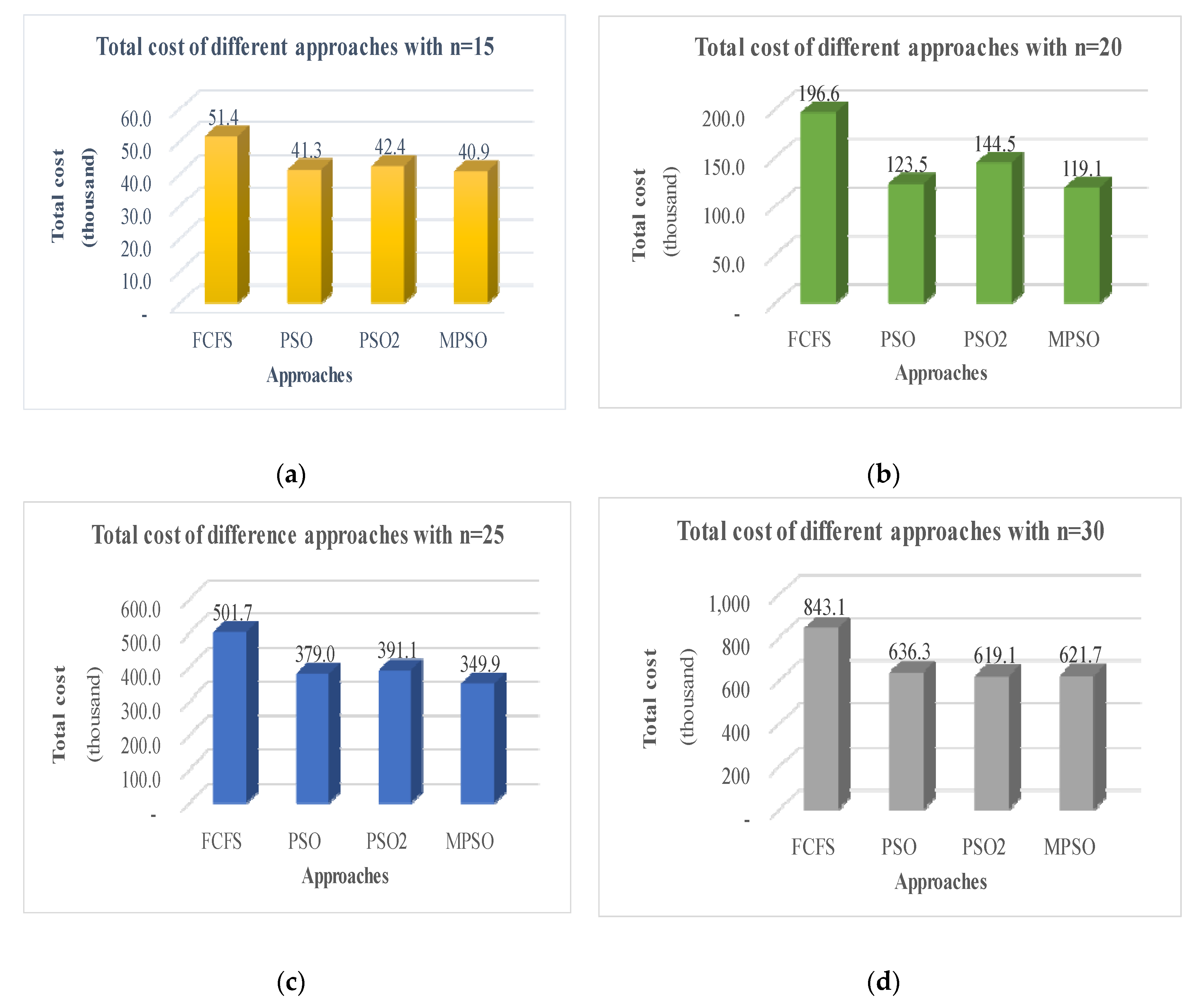
- This research has, respectively, employed FCFS, PSO, PSO2, and MPSO in the first stage of the two-stage procedure and it is found that these approaches lead to different results. The MPSO is found to outperform the other approaches in terms of the total cost defined in the objective function.
- (2)
- The tuning of the total number of iterative runs can also control the computational times. The more the iterative runs the more the computational times.
- (3)
- Although having less computational cost, the FCFS is incapable of finding a high-quality solution due to its simplicity. This disadvantage increases when the solution space increases. The FCFS cannot improve the solution continuously.
- (4)
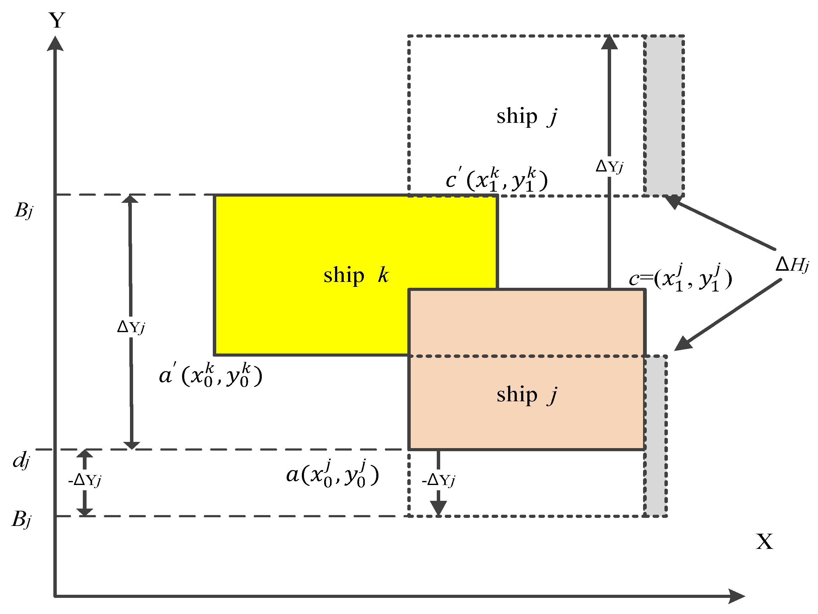
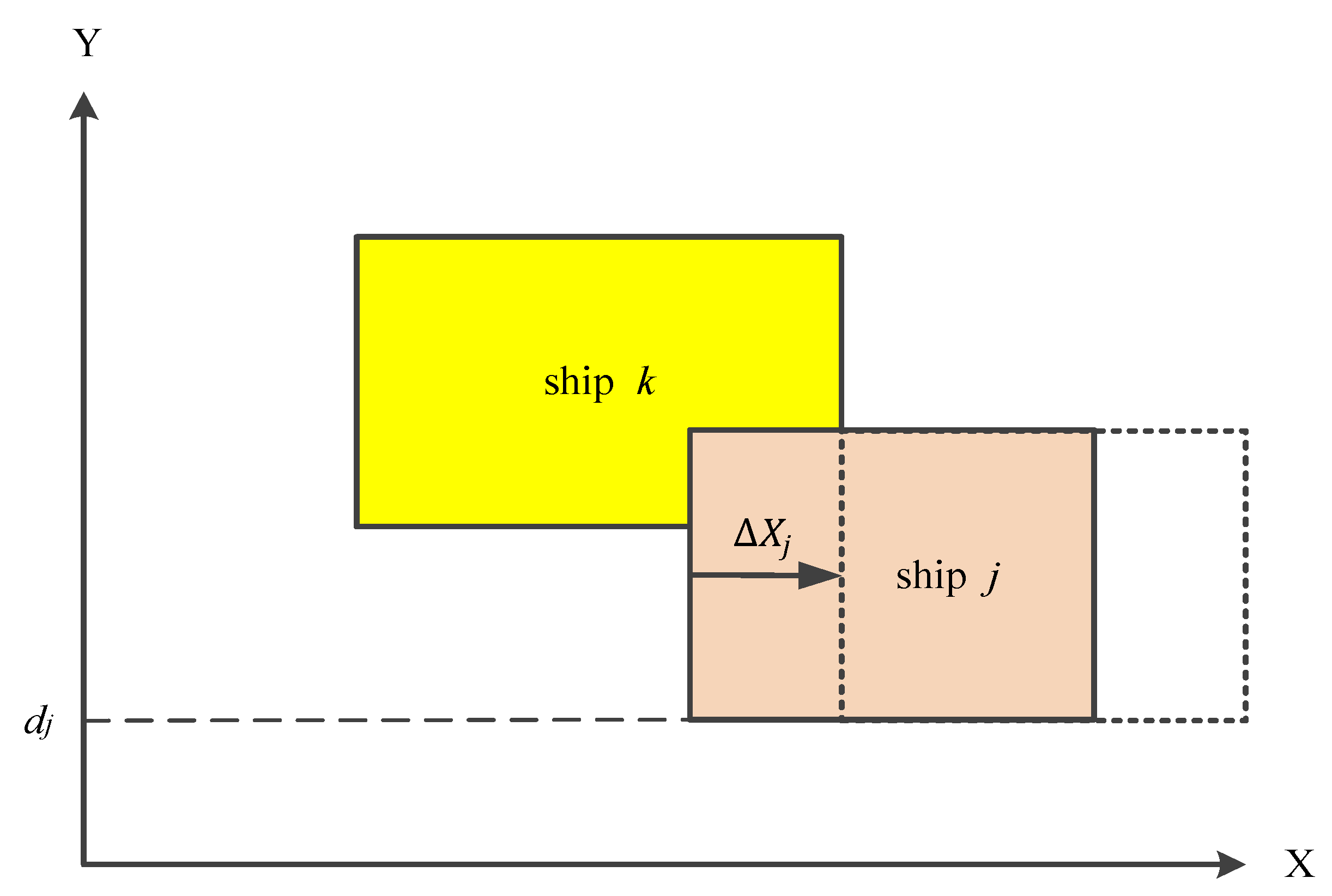
- It is found that moving a target toward either the +Y or −Y direction is less costly than towards the +X direction. This leads to the better use of available quay space. Thus, the cost values of C1 and C2 can inference the selection of a moving direction for a target ship.
- (5)
- As the least-cost direction has a high priority to be selected for a target ship, it is expected that our approach is likely to find, at least, a near-optimal solution. This cost estimation mechanism plays an essential role for this finding.
- (6)
- From Table 6, as the computational times to find the solutions for these approaches are found to be acceptable, these approaches are considered as applicable for practical usage.
- (7)
- Our approach is different from some proposed in past studies. For example, it differs from [39] in which the marginal decreasing capacity of QCs was not considered. This research differs from studies [5,18,19], which are PSO-based research. The [5] focused on a discrete version of BAP instead of a continuous version. The [18,19] only focused on the BAP, which did not consider the QCAP.
- (8)
- In [5] the proposed approach, PSO2, assigns a random number of QCs to a ship initially. However, this initial assignment cannot guarantee the best assignment of QCs to a ship as it did not use the . In this research, the MPSO assigns an initial number of QCs to a ship based on the , which promises the best assignment. The best number is to be adjusted if not conforming to the two QC constraints, Equations (8) and (9), to ensure a feasible solution. The experimental results show that the MPSO outperforms the PSO2 proposed in [5].
- (9)
- However, one limitation of the MPSO is that it cannot identify each QC assigned to a ship though it allows QC adjustment, i.e., it is the type of variable-in-time QCAP (number) instead of variable-in-time QCAP (specific) that is more specific and convenient for practical usage. Thus, there is room to improve the MPSO further.
- (10)
- One lack of this research is the comparison of the MPSO to GAs that have been widely used for solving seaside operational problems. This can be treated as a future research direction. Nevertheless, this research has achieved a preliminary result.
- (11)
- Although we have reached the preliminary conclusion that the MPSO outperforms the other approaches, extensive experiments are still required to consolidate this conclusion further.
- (12)
- One concern raised by a maritime supply chain is the damage and pollution to our environment, thus environmental protection is a concern. To pursuit higher efficiency for container terminal operations, some recent ideas have even proposed to allow speeding up ships so that they can arrive at a port earlier to make a better plan for resource usage (such as better use of quay space). However, speeding up a ship can introduce more air pollution that can damage our environment. In this research, speeding up a ship is not considered, as our approach does not allow a ship to move toward the −X direction (which requires a ship to speed up its speed). Thus, our approach has the merit of protecting our environment, while trying to better use resources including quay space and berths.
6. Conclusions
- (1)
- We have formulated the two problems as a mathematical model. Based on this model, a two-stage procedure was proposed to solve the two problems by including heuristics and metaheuristics.
- (2)
- A resolution of the conflict of ships is developed based on the concept of moving a target towards the least direction. This mechanism can lead to the finding of the optimal/near optimal solutions.
- (3)
- We have implemented this two-stage procedure by using java programing language to facilitate the generation of solutions. Our experiments show that our approach can find the optimal/near-optimal solution with acceptable computation times.
Author Contributions
Funding
Conflicts of Interest
References
- Zhen, L.; Yu, S.; Wang, S.; Sun, Z. Scheduling quay cranes and yard trucks for unloading operations in container ports. Ann. Oper. Res. 2019, 273, 455–478. [Google Scholar] [CrossRef]
- Bierwirth, C.; Meisel, F. A survey of berth allocation and quay crane scheduling problems in container terminals. EJOR 2010, 202, 615–627. [Google Scholar] [CrossRef]
- Vis, I.F.A.; Koster, R.D. Transshipment of container at a container terminal: An overview. EJOR 2003, 147, 1–16. [Google Scholar] [CrossRef]
- Raa, B.; Dullaert, W.; Schaeren, R.V. An enriched model for the integrated berth allocation and quay crane assignment problem. Expert Syst. Appl. 2011, 38, 14136–14147. [Google Scholar] [CrossRef]
- Hsu, H.P. A HPSO for solving dynamic and discrete berth allocation problem and dynamic quay crane assignment problem simultaneously. Swarm Evol. Comput. 2016, 27, 156–168. [Google Scholar] [CrossRef]
- Kim, K.H.; Moon, K.C. Berth scheduling by simulated annealing. Transp. Res. Part B 2003, 37, 541–560. [Google Scholar] [CrossRef]
- Salido, M.A.; Mario, R.M.; Barber, F. A decision support system for managing combinatorial problems in a container terminal. Knowl.-Based Syst. 2011, 29, 63–74. [Google Scholar] [CrossRef]
- Hsu, H.P.; Chiang, T.L. An Improved Shuffled Frog-Leaping Algorithm for Solving the Dynamic and Continuous Berth Allocation Problem (DCBAP). Appl. Sci. 2019, 9, 4682. [Google Scholar] [CrossRef]
- Leonora, B.; Dorigo, M.; Gambardella, L.M.; Gutjahr, W.J. A survey on metaheuristics for stochastic combinatorial optimization. Nat. Comput. Int. J. 2009, 8, 239–287. [Google Scholar]
- Liang, C.J.; Huang, Y.F.; Yang, Y. A quay crane dynamic scheduling problem by hybrid evolutionary algorithm for berth allocation planning. Comput. Ind. Eng. 2009, 56, 1021–1028. [Google Scholar] [CrossRef]
- Han, X.L.; Lu, Z.Q.; Xi, L.F. A proactive approach for simultaneous berth and quay crane scheduling problem with stochastic arrival and handling time. EJOR 2010, 207, 1327–1340. [Google Scholar] [CrossRef]
- Chang, D.F.; Jiang, Z.H.; Yan, W.; He, J.L. Integrating berth allocation and quay crane assignments. Transp. Res. Part E 2010, 46, 975–990. [Google Scholar] [CrossRef]
- Liang, C.J.; Guo, J.Q.; Yang, Y. Multi-objective hybrid genetic algorithm for quay crane dynamic assignment in birth allocation planning. J. Intell. Manuf. 2011, 22, 471–479. [Google Scholar] [CrossRef]
- Imai, A.; Etsuko, N.; Papadimitriou, S. Marine container terminal configurations for efficient handling of mega-containerships. Transp. Res. Part E Logist. Transp. Rev. 2013, 49, 141–158. [Google Scholar] [CrossRef]
- Rodriguez-Molins, M.; Ingolotti, L.; Barber, F.; Salido, M.A.; Sierra, M.R.; Puente, J. A genetic algorithm for robust berth allocation and quay crane assignment. Prog. Artif. Intell. 2014, 2, 177–192. [Google Scholar] [CrossRef]
- Hsu, H.P. A Hybrid GA with Variable Quay Crane Assignment for Solving Berth Allocation Problem and Quay Crane Assignment Problem Simultaneously. Sustainability 2019, 11, 2018. [Google Scholar] [CrossRef]
- Wang, F.; Lim, A. A stochastic beam search for the berth allocation problem. Decis. Support Syst. 2007, 42, 2186–2196. [Google Scholar] [CrossRef]
- Ting, C.J.; Wu, K.C.; Chou, H. Particle swarm optimization algorithm for the berth allocation problem. Expert Syst. Appl. 2014, 41, 543–1550. [Google Scholar] [CrossRef]
- Babazadeh, A.; Shahbandi, A.G.; Ganji, S.S.; Joharianzadeh, M. A PSO algorithm for continuous berth allocation problem. Int. J. Shipp. Transp. Logist. 2015, 7, 479. [Google Scholar] [CrossRef]
- Bierwirth, C.; Meisel, F. A follow-up survey of berth allocation and quay crane scheduling problems in container terminals. Eur. J. Oper. Res. 2015, 244, 675–689. [Google Scholar] [CrossRef]
- Kennedy, J.; Eberhart, R.C. Particle swarm optimization. In Proceedings of the IEEE International Conference on Neural Networks, Piscataway, NJ, USA, 27 November–1 December 1995; pp. 1942–1948. [Google Scholar]
- Allahverdi, A.; Al-Anzi, F.S. A PSO and a Tabu search heuristics for the assembly scheduling problem of the two-stage distributed data application. Comput. Oper. Res. 2006, 33, 1056–1080. [Google Scholar] [CrossRef]
- Zhou, P.F.; Kang, H.G. Study on Berth and Quay-crane Allocation under Stochastic Environments in Container Terminal. Syst. Eng.-Theory Pract. 2008, 28, 161–169. [Google Scholar] [CrossRef]
- Lin, S.Y.; Horng, S.J.; Dao, T.W.; Huang, D.K.; Fahn, C.S.; Lai, J.L.; Chen, R.J.; Kuo, I.H. Efficient bi-objective personnel assignment algorithm based on a hybrid particle swarm optimization model. Expert Syst. Appl. 2010, 37, 7825–7830. [Google Scholar] [CrossRef]
- Zhen, L.; Hu, H.; Wang, W.; Shi, X.; Ma, C. Cranes scheduling in frame bridges based automated container terminals. Transp. Res. Part C Emerg. Technol. 2018, 97, 369–384. [Google Scholar] [CrossRef]
- Liu, B.; Wang, L.; Jin, Y.H. An effective hybrid PSO-based algorithm for flow shop scheduling with limited buffers. Comput. Oper. Res. 2008, 35, 2791–2806. [Google Scholar] [CrossRef]
- Yuan, X.H.; Wang, L.; Yuan, Y.B. Application of enhanced PSO approach to optimal scheduling of hydro system. Energy Convers. Manag. 2008, 49, 2966–2972. [Google Scholar] [CrossRef]
- Zhou, D.W.; Gao, X.A.; Liu, G.H.; Mei, C.L.; Jiang, D.; Liu, Y. Randomization in particle swarm optimization for global search ability. Expert Syst. Appl. 2011, 38, 15356–15364. [Google Scholar] [CrossRef]
- Lee, D.H.; Wang, H.Q. Integrated discrete berth allocation and quay crane scheduling in port container terminals. Eng. Optim. 2010, 42, 747–761. [Google Scholar] [CrossRef]
- Lim, A. The berth scheduling problem. Oper. Res. Lett. 1998, 22, 105–110. [Google Scholar] [CrossRef]
- Lee, Y.; Chen, C.Y. An optimization heuristic for the berth scheduling problem. EJOR 2009, 196, 500–508. [Google Scholar] [CrossRef]
- Zhen, L.; Hay, L.H.; Chew, E.P. A decision model for berth allocation under uncertainty. EJOR 2011, 212, 54–68. [Google Scholar] [CrossRef]
- Imai, A.; Nishimura, E.; Paradimitrious, S. Corrigendum. The dynamic berth allocation problem for a container port. Transp. Res. Part B 2005, 39, 197. [Google Scholar] [CrossRef][Green Version]
- Meisel, F.; Bierwirth, C. Heuristic for the integration of crane productivity in the berth allocation problem. Transp. Res. Part E 2009, 45, 196–209. [Google Scholar] [CrossRef]
- Chang, D.F.; Yan, W.; Chen, C.H.; Jiang, Z.H. A berth allocation strategy using heuristics algorithm and simulation optimization. Int. J. Comput. Appl. Technol. 2008, 32, 272–281. [Google Scholar] [CrossRef]
- Zhang, C.R.; Zheng, L.; Zhang, Z.H.; Shi, L.Y.; Armstrong, A.J. The allocation of berths and quay cranes by using a sub-gradient optimization technique. Comput. Ind. Eng. 2010, 58, 40–50. [Google Scholar] [CrossRef]
- Yang, C.; Wang, X.; Li, Z. An optimization approach for coupling problem of berth allocation and quay crane assignment in container terminal. Comput. Ind. Eng. 2012, 62, 119–128. [Google Scholar] [CrossRef]
- Türkoğvllari, Y.B.; Taşkın, Z.C.; Aras, N.; Altınel, K. Optimal berth allocation and time-invariant quay crane assignment in container terminals. Eur. J. Oper. Res. 2014, 235, 88–101. [Google Scholar] [CrossRef]
- Park, Y.M.; Kim, K.H. A scheduling method for Berth and Quay cranes. OR Spectr. 2003, 25, 1–13. [Google Scholar] [CrossRef]


| Parameters | FCFS | PSO | PSO2 | MPSO |
|---|---|---|---|---|
| t | 1 | 20 | 20 | 20 |
| w | 0.5 | |||
| p | 64 | 64 | 64 | 64 |
| c1 | 2.0 | |||
| c2 | 2.0 | |||
| r1 | Random() | |||
| r2 | Random() | |||
| w1 | Equation defined in [5] | |||
| w2 | Equation defined in [5] | |||
| w3 | Equation defined in [5] | |||
| δ | 0.5 | |||
| θ | 0.5 | |||
| Rc | 0.3 | |||
| Rm | 0.4 | |||
| vmax | 2 | 2 | ||
| vmin | −2 | −2 | ||
| T0 | 90 | |||
| Te | 0 | |||
| β | 0.8 |
| No | SID | lj | dj | Cj | Lower-Left Hand Corner | Upper-Right Hand Corner | |||
|---|---|---|---|---|---|---|---|---|---|
| X0 | Y0 | X1 | Y1 | ||||||
| 1 | 3 | 167 | 26.1 | 398 | 1838 | 26.1 | 398 | 50.61 | 565 |
| 2 | 8 | 118 | 128.8 | 151 | 844 | 128.8 | 151 | 140.05 | 269 |
| 3 | 10 | 109 | 148.2 | 267 | 1080 | 148.2 | 267 | 162.60 | 376 |
| 4 | 1 | 108 | 147.3 | 169 | 1830 | 147.3 | 169 | 171.70 | 277 |
| 5 | 15 | 135 | 112.5 | 167 | 1768 | 112.5 | 167 | 136.07 | 302 |
| 6 | 4 | 134 | 89.5 | 344 | 864 | 89.5 | 344 | 101.02 | 478 |
| 7 | 9 | 154 | 42.8 | 574 | 1181 | 42.8 | 574 | 58.55 | 728 |
| 8 | 13 | 163 | 14.6 | 134 | 1759 | 14.6 | 134 | 38.05 | 297 |
| 9 | 7 | 131 | 33.3 | 272 | 1059 | 33.3 | 272 | 47.42 | 403 |
| 10 | 6 | 119 | 77.6 | 639 | 1152 | 77.6 | 639 | 92.96 | 758 |
| 11 | 12 | 158 | 35.8 | 582 | 1820 | 35.8 | 582 | 60.07 | 740 |
| 12 | 11 | 176 | 142.9 | 68 | 1820 | 142.9 | 68 | 160.89 | 244 |
| 13 | 2 | 165 | 140.1 | 602 | 1290 | 140.1 | 602 | 157.30 | 767 |
| 14 | 14 | 157 | 53.8 | 254 | 1267 | 53.8 | 254 | 70.69 | 411 |
| 15 | 5 | 184 | 126.4 | 592 | 1267 | 126.4 | 592 | 146.69 | 776 |
| Approaches | ||||
|---|---|---|---|---|
| Item | FCFS | PSO | PSO2 | MPSO |
| ΔWC | 61,551.1 | 24,758.2 | 55,740.8 | 18,345.6 |
| ΔHC | 11,030.0 | 15,369.2 | 14,660.0 | 19,133.9 |
| Z (Total cost) | 72,581.1 | 40,127.4 | 70,400.8 | 37479.5 |
| T (Times) | 1.57 s | 1.57 s | 1.57 s | 129.063 s |
| No | Ship id | lj | aj | dj | Cj | Lower-Left Hand Corner | Upper-Right Hand Corner | ΔWC | ΔHC | ||
|---|---|---|---|---|---|---|---|---|---|---|---|
| X0 | Y0 | X1 | Y1 | ||||||||
| 1 | 3 | 167 | 26.1 | 398 | 1838 | 26.1 | 398 | 50.61 | 565 | 0 | 0 |
| 2 | 8 | 118 | 128.8 | 151 | 844 | 128.8 | 151 | 142.48 | 269 | 0 | 2426.67 |
| 3 | 10 | 109 | 148.2 | 267 | 1080 | 158.09 | 267 | 173.85 | 376 | 9892.22 | 1357.04 |
| 4 | 1 | 108 | 147.3 | 169 | 1830 | 147.3 | 376 | 175.3 | 484 | 0 | 3597.41 |
| 5 | 15 | 135 | 112.5 | 167 | 1768 | 112.5 | 269 | 136.1 | 404 | 0 | 34 |
| 6 | 4 | 134 | 89.5 | 344 | 864 | 89.5 | 344 | 101.02 | 478 | 0 | 0 |
| 7 | 9 | 154 | 42.8 | 574 | 1181 | 49 | 574 | 65.29 | 728 | 6203.33 | 532.22 |
| 8 | 13 | 163 | 14.6 | 134 | 1759 | 14.6 | 134 | 38.05 | 297 | 0 | 0 |
| 9 | 7 | 131 | 33.3 | 272 | 1059 | 33.3 | 565 | 49 | 696 | 0 | 1583.33 |
| 10 | 6 | 119 | 77.6 | 639 | 1152 | 77.6 | 639 | 92.96 | 758 | 0 | 0 |
| 11 | 12 | 158 | 35.8 | 582 | 1820 | 38.05 | 240 | 65.97 | 298 | 2250 | 3647.78 |
| 12 | 11 | 176 | 142.9 | 68 | 1349 | 142.9 | 68 | 162.16 | 244 | 0 | 1273.33 |
| 13 | 2 | 165 | 140.1 | 602 | 1290 | 140.1 | 602 | 158.09 | 767 | 0 | 792.22 |
| 14 | 14 | 157 | 53.8 | 254 | 1267 | 53.8 | 398 | 74.52 | 555 | 0 | 3831.85 |
| 15 | 5 | 184 | 126.4 | 592 | 1525 | 126.4 | 418 | 146.7 | 602 | 0 | 58 |
| Sub-total | 18,345.6 | 19,133.9 | |||||||||
| Total () | 37,479.5 | ||||||||||
| No | Fm | To | SID | S | Ship ID | ||||||||||||||
|---|---|---|---|---|---|---|---|---|---|---|---|---|---|---|---|---|---|---|---|
| 1 | 2 | 3 | 4 | 5 | 6 | 7 | 8 | 9 | 10 | 11 | 12 | 13 | 14 | 15 | |||||
| 1 | 0 | 14.6 | 13 | 2 | 3 | ||||||||||||||
| 2 | 14.6 | 26.1 | 3 | 2 | 3 | 3 | |||||||||||||
| 3 | 26.1 | 33.3 | 7 | 2 | 3 | 2 | 3 | ||||||||||||
| 4 | 33.3 | 38 | 13 | 3 | 3 | 3 | |||||||||||||
| 5 | 38 | 38 | 12 | 2 | 3 | 3 | 2 | ||||||||||||
| 6 | 38 | 49 | 7 | 3 | 3 | 3 | |||||||||||||
| 7 | 49 | 49 | 9 | 2 | 3 | 2 | 3 | ||||||||||||
| 8 | 49 | 50.6 | 3 | 3 | 3 | 3 | |||||||||||||
| 9 | 50.6 | 53.8 | 14 | 2 | 3 | 3 | 2 | ||||||||||||
| 10 | 53.8 | 65.3 | 9 | 3 | 3 | 3 | |||||||||||||
| 11 | 65.3 | 66 | 12 | 3 | 3 | ||||||||||||||
| 12 | 66 | 74.5 | 14 | 3 | |||||||||||||||
| 13 | 74.5 | 77.6 | 6 | 2 | 3 | ||||||||||||||
| 14 | 77.6 | 89.5 | 4 | 2 | 3 | 3 | |||||||||||||
| 15 | 89.5 | 93 | 6 | 3 | 3 | ||||||||||||||
| 16 | 93 | 101 | 4 | 3 | |||||||||||||||
| 17 | 101 | 112.5 | 15 | 2 | 3 | ||||||||||||||
| 18 | 112.5 | 126.4 | 5 | 2 | 3 | 3 | |||||||||||||
| 19 | 126.4 | 128.8 | 8 | 2 | 3 | 2 | 3 | ||||||||||||
| 20 | 128.8 | 136.1 | 15 | 3 | 3 | 3 | |||||||||||||
| 21 | 136.1 | 140.1 | 2 | 2 | 2 | 3 | 3 | ||||||||||||
| 22 | 140.1 | 142.5 | 8 | 3 | 3 | 3 | |||||||||||||
| 23 | 142.5 | 142.9 | 11 | 2 | 3 | 3 | 2 | ||||||||||||
| 24 | 142.9 | 146.7 | 5 | 3 | 3 | 3 | |||||||||||||
| 25 | 146.7 | 147.3 | 1 | 2 | 2 | 3 | 3 | ||||||||||||
| 26 | 147.3 | 158.1 | 2 | 3 | 3 | 3 | |||||||||||||
| 27 | 158.1 | 158.1 | 10 | 2 | 3 | 2 | 3 | ||||||||||||
| 28 | 158.1 | 162.2 | 11 | 3 | 3 | 3 | |||||||||||||
| 29 | 162.2 | 173.8 | 10 | 3 | 3 | ||||||||||||||
| 30 | 173.8 | 175.3 | 1 | 3 | |||||||||||||||
| FCFS | PSO | PSO2 | MPSO | |||||
|---|---|---|---|---|---|---|---|---|
| N = 15 | Z | T | Z | T | Z | T | Z | T |
| 1 | 64,683.7 | 0.4 | 64,683.7 | 13.0 | 71,372.2 | 16.3 | 61,707.0 | 137.2 |
| 2 | 43,463.3 | 0.4 | 27,335.5 | 8.4 | 27,335.5 | 12.1 | 27,335.5 | 79.7 |
| 3 | 35,920.3 | 0.4 | 32,518.1 | 11.2 | 32,518.1 | 17.7 | 32,518.1 | 120.7 |
| 4 | 78,542.8 | 0.4 | 44,180.8 | 13.0 | 44,180.8 | 21.4 | 44,180.8 | 143.9 |
| 5 | 33,372.2 | 0.4 | 31,381.1 | 9.2 | 31,923.3 | 13.2 | 31,381.1 | 97.6 |
| 6 | 37,798.1 | 0.4 | 37,798.1 | 13.2 | 37,798.1 | 17.0 | 37,798.1 | 149.3 |
| 7 | 58,942.9 | 0.4 | 58,927.1 | 13.2 | 61,305.4 | 20.9 | 57,407.6 | 150.7 |
| 8 | 33,090.0 | 0.4 | 18,567.7 | 9.4 | 18,567.7 | 13.2 | 18,567.7 | 92.2 |
| 9 | 49,148.5 | 0.4 | 46,223.3 | 16.2 | 46,801.8 | 18.4 | 46,223.3 | 134.1 |
| 10 | 78,829.2 | 0.4 | 51,495.9 | 9.7 | 51,630.1 | 20.2 | 51,495.9 | 102.6 |
| Avg. | 51,379.1 | 0.4 | 41,311.1 | 11.7 | 42,399.0 | 17.0 | 40,861.5 | 120.8 |
| N = 20 | Z | T | Z | T | Z | T | Z | T |
| 1 | 52,850.0 | 0.3 | 48,371.1 | 14.8 | 52,850.0 | 21.4 | 48,371.1 | 158.6 |
| 2 | 130,274.7 | 0.4 | 78,144.0 | 17.1 | 102,875.5 | 25.9 | 71,693.9 | 198.3 |
| 3 | 78,635.2 | 0.4 | 52,986.3 | 15.6 | 52,986.3 | 22.0 | 52,986.3 | 178.5 |
| 4 | 218,097.7 | 0.3 | 162,495.5 | 14.2 | 140,255.0 | 30.7 | 149,887.0 | 159.2 |
| 5 | 315,525.4 | 0.4 | 173,686.9 | 19.5 | 196,587.5 | 31.5 | 176,399.1 | 220.9 |
| 6 | 399,651.6 | 0.3 | 176,799.2 | 19.7 | 261,978.7 | 29.7 | 173,919.3 | 221.0 |
| 7 | 228,430.4 | 0.4 | 105,253.6 | 17.1 | 172,601.2 | 24.2 | 96,449.2 | 194.8 |
| 8 | 70,074.1 | 0.3 | 69,024.8 | 16.1 | 79,974.6 | 25.1 | 66,469.3 | 185.8 |
| 9 | 129,956.7 | 0.3 | 84,379.7 | 15.3 | 97,594.0 | 22.4 | 83,122.3 | 170.4 |
| 10 | 342,539.1 | 0.3 | 283,706.5 | 15.5 | 287,765.3 | 26.8 | 272,191.9 | 172.4 |
| Avg. | 196,603.5 | 0.3 | 123,484.8 | 16.5 | 144,546.8 | 26.0 | 119,148.9 | 186.0 |
| N = 25 | Z | T | Z | T | Z | T | Z | T |
| 1 | 519,044.0 | 0.4 | 319,344.3 | 27.1 | 360,801.4 | 73.8 | 301,731.1 | 461.5 |
| 2 | 417,073.2 | 0.4 | 356,883.6 | 43.9 | 339,845.3 | 63.8 | 326,855.9 | 362.6 |
| 3 | 968,779.5 | 0.4 | 679,711.5 | 33.1 | 606,488.8 | 73.7 | 659,997.3 | 1441.6 |
| 4 | 383,264.7 | 0.4 | 279,950.7 | 60.0 | 349,901.0 | 105.1 | 263,709.6 | 912.4 |
| 5 | 322,685.3 | 0.8 | 208,590.6 | 66.0 | 284,606.1 | 251.1 | 212,131.9 | 839.9 |
| 6 | 529,640.8 | 0.6 | 487,985.8 | 50.5 | 559,947.5 | 117.5 | 329,771.0 | 1049.8 |
| 7 | 225,380.0 | 0.4 | 146,537.4 | 26.6 | 156,685.9 | 58.8 | 137,635.2 | 746.5 |
| 8 | 329,470.8 | 0.3 | 312,931.8 | 40.3 | 325,643.4 | 64.7 | 288,524.7 | 341.8 |
| 9 | 794,016.0 | 0.4 | 609,751.5 | 34.2 | 554,842.2 | 99.1 | 601,662.3 | 815.0 |
| 10 | 527,476.6 | 0.4 | 388,389.2 | 69.5 | 372,384.8 | 40.6 | 377,306.5 | 301.6 |
| Avg. | 501,683.1 | 0.4 | 379,007.6 | 45.1 | 391,114.6 | 94.8 | 349,932.6 | 727.3 |
| N = 30 | Z | T | Z | T | Z | T | Z | T |
| 1 | 280,309.3 | 0.3 | 192,679.5 | 22.8 | 264,531.4 | 38.3 | 152,391.4 | 261.9 |
| 2 | 219,780.4 | 0.4 | 122,902.1 | 23.5 | 169,330.9 | 36.3 | 126,911.9 | 267.7 |
| 3 | 191,652.2 | 0.4 | 99,641.6 | 20.9 | 137,728.7 | 38.4 | 91,690.0 | 233.9 |
| 4 | 326,444.1 | 0.4 | 212,452.8 | 23.2 | 251,530.4 | 45.0 | 203,730.3 | 263.7 |
| 5 | 1,638,434.5 | 0.4 | 1,245,954.6 | 34.5 | 1,306,552.2 | 81.9 | 1,281,544.0 | 430.2 |
| 6 | 1,241,025.7 | 0.4 | 1,173,821.3 | 35.3 | 1,027,884.1 | 84.5 | 1,169,000.7 | 436.2 |
| 7 | 1,509,662.9 | 0.4 | 973,022.3 | 37.0 | 853,598.5 | 91.4 | 940,819.3 | 440.2 |
| 8 | 688,383.0 | 0.4 | 602,804.1 | 46.7 | 521,229.2 | 106.8 | 553,369.4 | 1,312.4 |
| 9 | 1,368,850.4 | 0.4 | 1,018,128.0 | 34.7 | 919,646.3 | 106.4 | 1,003,536.2 | 471.0 |
| 10 | 966,228.0 | 0.4 | 721,914.3 | 131.5 | 655,321.0 | 122.9 | 693,514.7 | 870.5 |
| Avg. | 843,077.0 | 0.4 | 636,332.1 | 41.0 | 619,124.2 | 75.2 | 621,650.8 | 498.8 |
© 2020 by the authors. Licensee MDPI, Basel, Switzerland. This article is an open access article distributed under the terms and conditions of the Creative Commons Attribution (CC BY) license (http://creativecommons.org/licenses/by/4.0/).
Share and Cite
Hsu, H.-P.; Wang, C.-N. Resources Planning for Container Terminal in a Maritime Supply Chain Using Multiple Particle Swarms Optimization (MPSO). Mathematics 2020, 8, 764. https://doi.org/10.3390/math8050764
Hsu H-P, Wang C-N. Resources Planning for Container Terminal in a Maritime Supply Chain Using Multiple Particle Swarms Optimization (MPSO). Mathematics. 2020; 8(5):764. https://doi.org/10.3390/math8050764
Chicago/Turabian StyleHsu, Hsien-Pin, and Chia-Nan Wang. 2020. "Resources Planning for Container Terminal in a Maritime Supply Chain Using Multiple Particle Swarms Optimization (MPSO)" Mathematics 8, no. 5: 764. https://doi.org/10.3390/math8050764
APA StyleHsu, H.-P., & Wang, C.-N. (2020). Resources Planning for Container Terminal in a Maritime Supply Chain Using Multiple Particle Swarms Optimization (MPSO). Mathematics, 8(5), 764. https://doi.org/10.3390/math8050764