On a Periodic Capital Injection and Barrier Dividend Strategy in the Compound Poisson Risk Model

Abstract

In this paper, we assume that the reserve level of an insurance company can only be observed at discrete time points, then a new risk model is proposed by introducing a periodic capital injection strategy and a barrier dividend strategy into the classical risk model. We derive the equations and the boundary conditions satisfied by the Gerber-Shiu function, the expected discounted capital injection function and the expected discounted dividend function by assuming that the observation interval and claim amount are exponentially distributed, respectively. Numerical examples are also given to further analyze the influence of relevant parameters on the actuarial function of the risk model.

1. Introduction

In the classical risk model, the reserve process of an insurance ${\left\{U(t)\right\}}_{t\ge 0}$ has the following form,

$$\begin{array}{c}\hfill U(t)=u+ct-S(t)=u+ct-{\displaystyle \sum _{k=1}^{N(t)}}{Y}_k,t\ge 0,\end{array}$$

(1)

where the initial reserve is $U(0)=u$, the parameter $c>0$ is the incoming premium rate per unit time, the aggregate claims process $S(t)={\sum }_{k=1}^{N(t)}{Y}_k$ is a compound Poisson process, where the Poisson process ${\left\{N(t)\right\}}_{t\ge 0}$ is the number of claims up to time t with intensity $\lambda >0$, claim amount ${\left\{Y_k\right\}}_{k=1}^{\infty }$ is a sequence of independent identically distributed random variables with common density $f_Y(y)$. ${\left\{N(t)\right\}}_{t\ge 0}$ and ${\left\{Y_k\right\}}_{k=1}^{\infty }$ are independent of each other.

The classical risk model and extended risk models, such as those with dividend, investment or capital injection strategy, all require insurance companies to continuously observe the reserve process, which will greatly increase the operating costs of insurance companies. Relevant literature can be consulted Chi and Lin [1], Yin et al. [2], Li and Lu [3], Zeng et al. [4,5], Yu et al. [6], Zhou et al. [7], Yu [8], Zhang et al. [9], Zhou et al. [10], Yu et al. [11], Xu et al. [12], Liu et al. [13], Peng and Wang [14], Wang et al. [15]. In order to reduce operating costs, insurance companies usually choose to observe reserve process regularly. Thus, the risk model under discrete-time observation emerges as the times require. Asmussen and Albrecher [16] study a series of compound Poisson risk models with discrete-time observations. Albrecher et al. [17,18] propose to observe reserve level only at some discrete time points, and assume that the observation interval obeys Erlang distribution, and study the risk model accordingly. Choi and Cheung [19] consider a generalized model in which ruin is monitored at all observation times whose intervals are Erlang(n) distributed, whereas dividend decisions are made at a subset of these times ruin is checked. Avanzi et al. [20] study a dual risk model with a dividend barrier strategy, in which the dividend decisions are made periodically whereas solvency is monitored continuously. Zhang et al. [21] propose a spectrally negative Lévy insurance risk model with periodic tax payments, and assume that the event of ruin is only checked at a sequence of Poisson arrival times. Zhang et al. [22] assume that capital injections are only allowed at a sequence of time points with inter-capital-injection times being Erlang distributed under a compound Poisson risk model. Cheung and Zhang [23] consider a compound Poisson risk model in which it is assumed that the insurer observes its reserve level periodically to decide on dividend payments at the arrival times of an Erlang(n) renewal process. Peng et al. [24] model the insurance company’s reserve flow by a perturbed compound Poisson model and suppose that at a sequence of random time points, the insurance company observes the reserve to decide dividend payments. Yang and Deng [25] study the discounted Gerber-Shiu type function for a perturbed risk model with interest and periodic dividend strategy. Other recent articles on risk models with dividend strategy and capital injection involving periodic observations can be found in Zhang and Liu [26], Zhang [27], Zhang and Han [28], Zhao et al. [29], Pérez and Yamazaki [30], Noba et al. [31], Dong and Zhou [32], Xu et al. [33], Zhang et al. [34], Liu and Yu [35], Zhang and Cheung [36], Yu et al. [37] and Liu and Zhang [38].

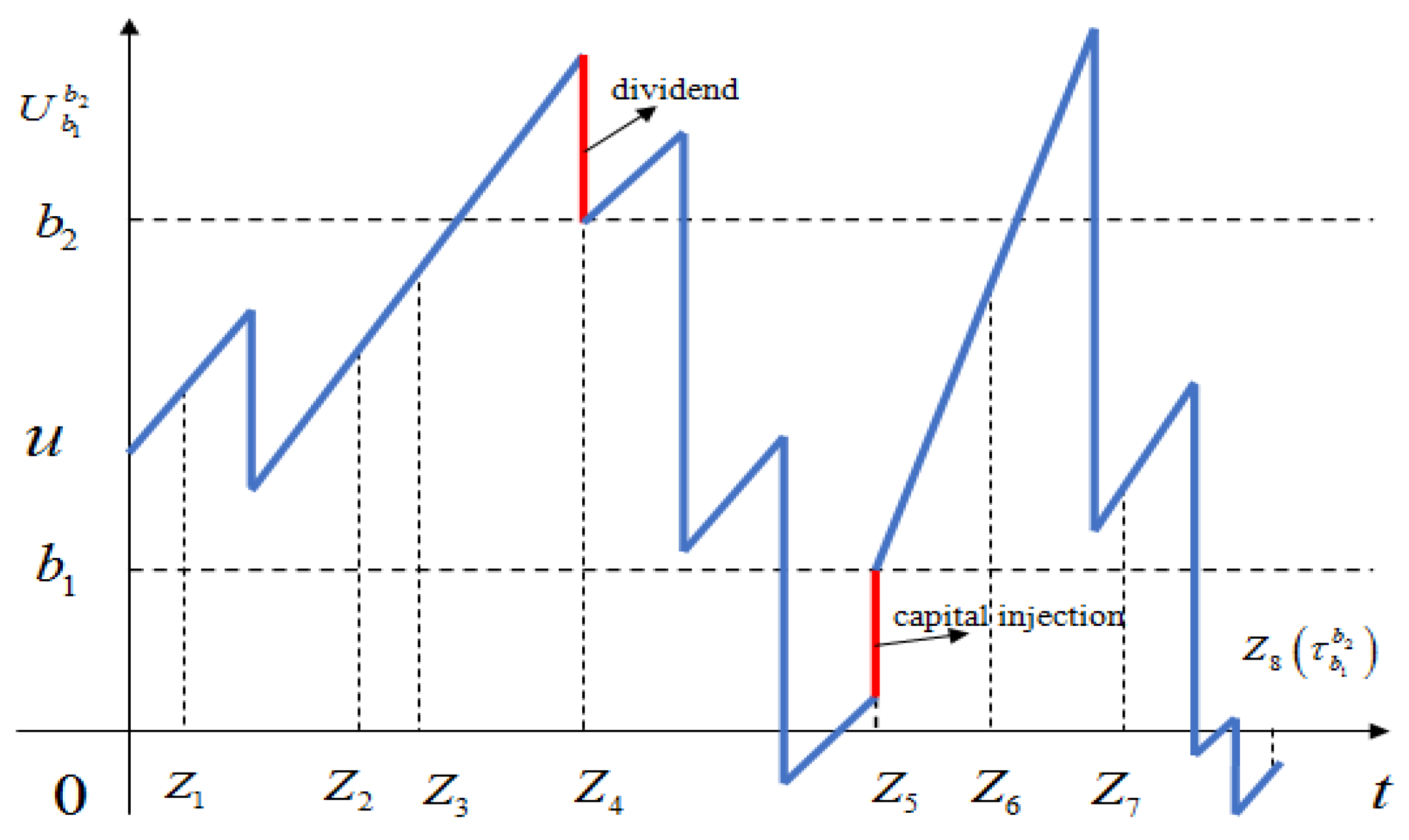
In this paper, considering the operating cost of insurance companies, we only observe the reserve level at the discrete time point ${\left\{Z_k\right\}}_{k=1}^{\infty }$. Let $T_k=Z_k-Z_{k-1}$, that is, the variable $T_k$ is the interval between the $(k-1)$th observation and the kth observation. It is assumed that ${\left\{T_k\right\}}_{k=1}^{\infty }$ is a series of independent and identically distributed random variables, and that ${\left\{T_k\right\}}_{k=1}^{\infty }$, ${\left\{N(t)\right\}}_{t\ge 0}$ and ${\left\{Y_k\right\}}_{k=1}^{\infty }$ are independent of each other. On the basis of this discrete assumption, we further study the introduction of capital injection and barrier dividend strategy. At the observational time point $Z_k$, if the reserve level is less than 0, ruin will be declared immediately. When the reserve level u is such that $u\in [0,b_1)$, it should be injected immediately to make its reserve reach the capital injection line $b_1$, that is, the amount of capital injection is $b_1-u$. When the reserve level is above the dividend line $b_2(b_2>b_1)$, the reserve that exceeds $b_2$ will be paid immediately, so that the reserve will return to $b_2$ immediately. In addition, in the absence of observation, no matter what the level of reserve, there will be no ruin declaration, capital injection, dividend payment and other acts (see Figure 1). Denoting the modified process of the new risk model with periodic capital injection and barrier dividend strategy as $U_{b_1}^{b_2}={\left\{U_{b_1}^{b_2}(t)\right\}}_{t\ge 0}$, its dynamics can be jointly described with the auxiliary processes ${\left\{U^{(k)}(t)\right\}}_{t\ge Z_{k-1}}$ by

$$U^{(k)}(t)=\left\{\begin{array}{cc}U(t),\hfill & k=1,t\ge 0,\hfill \\ U_{b_1}^{b_2}(Z_{k-1})+U(t)-U(Z_{k-1}),\hfill & k=2,3,\dots \dots ;t\ge Z_{k-1},\hfill \end{array}\right.$$

(2)

and for $k=1,2,3,\dots \dots$

$$U_{b_1}^{b_2}(t)=\left\{\begin{array}{cc}{U}^{(k)}(t),\hfill & Z_{k-1}<t<Z_k,\hfill \\ max\{U^{(k)}(Z_k),b_1\},\hfill & t=Z_k,U^{(k)}(Z_k)\le b_1,\hfill \\ min\{U^{(k)}(Z_k),b_2\},\hfill & t=Z_k,U^{(k)}(Z_k)\ge b_2,\hfill \\ U^{(k)}(Z_k),\hfill & t=Z_k,b_1<U^{(k)}(Z_k)<b_2.\hfill \end{array}\right.$$

(3)

Then, in the kth observation, the reserve level of the new risk model should be expressed as

$$\begin{array}{c}\hfill U_{b_1}^{b_2}(k)=U_{b_1}^{b_2}(k-1)+c{T}_k-[S(Z_k)-S(Z_{k-1})],k=1,2,3,\dots \end{array}$$

(4)

Without loss of generality, we assume that $Z_0=0-$. (i.e., time zero is not a capital injection time and dividend payment time.) So that the initial reserve level $U_{b_1}^{b_2}(0)=u$ even if $0<u<b_1$ or $u>b_2$. The ruin time ${\tau }_{b_1}^{b_2}$ is defined as ${\tau }_{b_1}^{b_2}=inf\{t\ge 0|U_{b_1}^{b_2}(t)<0\}$ with the convention $inf\varnothing =\infty$. Based on the assumption of the above model, the key quantity of interest in this paper is study of the Gerber-Shiu function, the expected discount injection function and the expected discount dividend function.

The Gerber-Shiu function is defined as follows:

$$\begin{array}{c}\hfill m_{\delta }(u;b_1,b_2)=\mathbb{E}\left[e^{-\delta {\tau }_{b_1}^{b_2}}\omega (U_{b_1}^{b_2}({\tau }_{b_1}^{b_2}-),|U_{b_1}^{b_2}({\tau }_{b_1}^{b_2})|)I_{\{{\tau }_{b_1}^{b_2}<\infty \}}|U_{b_1}^{b_2}(0)=u\right],\end{array}$$

(5)

where the parameter $\delta \ge 0$ is the force of interest, the symbol $I_A$ is the indicator function of the event A. The penalty function $w(x_1,x_2):[0,\infty )\times [0,\infty )\to [0,\infty )$ is a continuous nonnegative bounded penalty function of the reserve before ruin and the deficit at ruin. The Gerber-Shiu function was first proposed by Gerber and Shiu [39]. Since then, it has become a standard tool for studying ruin related quantities. We refer the interested readers to Lin et al. [40], Huang and Yu [41], Ruan et al. [42], Li et al. [43], Wang et al. [44], Yang et al. [45], Yu [46,47], Yuen et al. [48], Huang et al. [49], Xie and Zou [50].

The expected discount injection function is described by

$$\begin{array}{c}\hfill V_1(u;b_1,b_2)=\mathbb{E}\left[\sum _{k=1}^{\infty }{e}^{-\delta Z_k}{\chi }_1(b_1-U_{b_1}^{b_2}(Z_k))I_{\{Z_k<{\tau }_{b_1}^{b_2}\}}|U_{b_1}^{b_2}(0)=u\right],\end{array}$$

(6)

where the function ${\chi }_1(x)$ is a nonnegative function about the amount of capital injection for $x\in (0,b_1]$, and ${\chi }_1(x)=0$ for $x\le 0$.

The expected discount dividend function is defined as follows:

$$\begin{array}{c}\hfill V_2(u;b_1,b_2)=\mathbb{E}\left[\sum _{k=1}^{\infty }{e}^{-\delta Z_k}{\chi }_2(U_{b_1}^{b_2}(Z_{k-})-b_2)I_{\{Z_k<{\tau }_{b_1}^{b_2}\}}|U_{b_1}^{b_2}(0)=u\right],\end{array}$$

(7)

where the function ${\chi }_2(x)$ is a nonnegative function about the amount of dividends payment for $x>0$, and ${\chi }_2(x)=0$ for $x\le 0$.

The outline of the paper is organized as follows. In Section 2, we derive integro-differential equations for Gerber-Shiu function and give the explicit solution. Similarly, the expected discount injection function and the expected discount dividend function are studied in Section 3 and Section 4, respectively. In Section 5, some numerical examples are given to analyze the effect of relevant parameters on the actuarial function. Finally, Conclusions are given in Section 6.

2. Gerber-Shiu Function

In this section, we assume that the observational time interval $T_k$ and claim arrival time are exponentially distributed with parameters $\gamma$ and $\lambda$, respectively. It should be noted that this paper only considers that the penalty function only depends on the ruin deficit, that is $w(x_1,x_2)=w(x_2)$, where $w(x_2),(x_2\ge 0)$ is a continuous nonnegative bounded penalty function. On this basis, in the period of $(0,h)$, according to the observation of the reserve level and the occurrence of claims, the Gerber-Shiu function $m_{\delta }(u;b_1,b_2)$ satisfies the following integro equation.

$$\begin{array}{cc}\hfill m_{\delta }(u;b_1,b_2)& =e^{-(\delta +\lambda +\gamma )h}{m}_{\delta }(u+ch;b_1,b_2)+{\int }_0^h{e}^{-(\lambda +\delta )t}\gamma e^{-\gamma t}H(t)dt\hfill \\ \hfill & +{\int }_0^h{e}^{-(\delta +\gamma )t}\lambda e^{-\lambda t}{\int }_0^{\infty }{m}_{\delta }(u+ct-y;b_1,b_2)f_Y(y)dydt,\hfill \end{array}$$

(8)

where,

$$\begin{array}{cc}\hfill H(t)& =m_{\delta }(b_2;b_1,b_2)I_{\{u+ct>b_2\}}+m_{\delta }(u+ct;b_1,b_2)I_{\{b_1<u+ct⩽b_2\}}\hfill \\ \hfill & +m_{\delta }(b_1;b_1,b_2)I_{\{0⩽u+ct⩽b_1\}}+w(-(u+ct))I_{\{u+ct<0\}}.\hfill \end{array}$$

It is noted that if the claim occurs before the observation, the reserve level may be less than 0 without being observed. Therefore, the initial reserve $u\in \mathbb{R}$. The function $m_{\delta }(u;b_1,b_2)$ is a right continuous function defined on $\mathbb{R}$. According to Albrecher et al. [18], the function $m_{\delta }(u;b_1,b_2)$ is differentiable at $u\in \mathbb{R}$ except for zero. By taking the derivative of h on both sides of formula (8) at the same time and then making $h=0$, the following integro-differential equation satisfied by $m_{\delta }(u;b_1,b_2)$ can be obtained

$$\begin{array}{cc}\hfill 0=& -(\delta +\lambda +\gamma )m_{\delta }(u;b_1,b_2)+c{m}_{\delta }^{\prime }(u;b_1,b_2)+\lambda {\int }_0^{\infty }{m}_{\delta }(u-y;b_1,b_2)f_Y(y)dy\hfill \\ \hfill & +\gamma [m_{\delta }(b_2;b_1,b_2)I_{\{u>b_2\}}+m_{\delta }(u;b_1,b_2)I_{\{b_1<u⩽b_2\}}\hfill \\ \hfill & +m_{\delta }(b_1;b_1,b_2)I_{\{0⩽u⩽b_1\}}+w(-u)I_{\{u<0\}}].\hfill \end{array}$$

(9)

According to the different value range of u, formula (9) can be divided into

$$\begin{array}{cc}\hfill 0=& -(\delta +\lambda +\gamma )m_{\delta }(u;b_1,b_2)+c{m}_{\delta }^{\prime }(u;b_1,b_2)+\gamma m_{\delta }(b_2;b_1,b_2)\hfill \\ \hfill & +\lambda {\int }_0^{\infty }{m}_{\delta }(u-y;b_1,b_2)f_Y(y)dy,u>b_2,\hfill \end{array}$$

(10)

$$\begin{array}{cc}\hfill 0=& -(\delta +\lambda )m_{\delta }(u;b_1,b_2)+c{m}_{\delta }^{\prime }(u;b_1,b_2)\hfill \\ \hfill & +\lambda {\int }_0^{\infty }{m}_{\delta }(u-y;b_1,b_2)f_Y(y)dy,b_1<u\le b_2,\hfill \end{array}$$

(11)

$$\begin{array}{cc}\hfill 0=& -(\delta +\lambda +\gamma )m_{\delta }(u;b_1,b_2)+c{m}_{\delta }^{\prime }(u;b_1,b_2)+\gamma m_{\delta }(b_1;b_1,b_2)\hfill \\ \hfill & +\lambda {\int }_0^{\infty }{m}_{\delta }(u-y;b_1,b_2)f_Y(y)dy,0\le u\le b_1,\hfill \end{array}$$

(12)

$$\begin{array}{cc}\hfill 0=& -(\delta +\lambda +\gamma )m_{\delta }(u;b_1,b_2)+c{m}_{\delta }^{\prime }(u;b_1,b_2)+\gamma w(-u)\hfill \\ \hfill & +\lambda {\int }_0^{\infty }{m}_{\delta }(u-y;b_1,b_2)f_Y(y)dy,u<0.\hfill \end{array}$$

(13)

For the convenience of description, according to the range of values of u, the Gerber-Shiu function $m_{\delta }(u;b_1,b_2)$ is rewritten to

$${\displaystyle m_{\delta }(u;b_1,b_2):=\left\{\begin{array}{cc}{m}_{\delta ,U_1}(u;b_1,b_2),\hfill & u>b_2,\hfill \\ m_{\delta ,U_2}(u;b_1,b_2),\hfill & b_1<u\le b_2,\hfill \\ m_{\delta ,U_3}(u;b_1,b_2),\hfill & 0\le u\le b_1,\hfill \\ m_{\delta ,L}(u;b_1,b_2),\hfill & u<0.\hfill \end{array}\right.}$$

Thus, the integro-differential equations mentioned above can be divided into the following four cases:

When $u>b_2$,

$$\begin{array}{cc}\hfill 0=& -(\delta +\lambda +\gamma )m_{\delta ,U_1}(u;b_1,b_2)+c{m}_{\delta ,U_1}^{\prime }(u;b_1,b_2)+\gamma m_{\delta ,U_1}(b_2;b_1,b_2)\hfill \\ \hfill & +\lambda {\int }_0^{u-b_2}{m}_{\delta ,U_1}(u-y;b_1,b_2)f_Y(y)dy+\lambda {\int }_{u-b_2}^{u-b_1}{m}_{\delta ,U_2}(u-y;b_1,b_2)f_Y(y)dy\hfill \\ \hfill & +\lambda {\int }_{u-b_1}^u{m}_{\delta ,U_3}(u-y;b_1,b_2)f_Y(y)dy+\lambda {\int }_u^{\infty }{m}_{\delta ,L}(u-y;b_1,b_2)f_Y(y)dy,\hfill \end{array}$$

(14)

and when $b_1<u\le b_2$,

$$\begin{array}{cc}\hfill 0=& -(\delta +\lambda )m_{\delta ,U_2}(u;b_1,b_2)+c{m}_{\delta ,U_2}^{\prime }(u;b_1,b_2)+\lambda {\int }_0^{u-b_1}{m}_{\delta ,U_2}(u-y;b_1,b_2)f_Y(y)dy\hfill \\ \hfill & +\lambda {\int }_{u-b_1}^u{m}_{\delta ,U_3}(u-y;b_1,b_2)f_Y(y)dy+\lambda {\int }_u^{\infty }{m}_{\delta ,L}(u-y;b_1,b_2)f_Y(y)dy,\hfill \end{array}$$

(15)

and when $0<u\le b_1$,

$$\begin{array}{cc}\hfill 0=& -(\delta +\lambda +\gamma )m_{\delta ,U_3}(u;b_1,b_2)+c{m}_{\delta ,U_3}^{\prime }(u;b_1,b_2)+\gamma m_{\delta ,U_3}(b_1;b_1,b_2)\hfill \\ \hfill & +\lambda {\int }_0^u{m}_{\delta ,U_3}(u-y;b_1,b_2)f_Y(y)dy+\lambda {\int }_u^{\infty }{m}_{\delta ,L}(u-y;b_1,b_2)f_Y(y)dy,\hfill \end{array}$$

(16)

and when $u\le 0$,

$$\begin{array}{cc}\hfill 0=& -(\delta +\lambda +\gamma )m_{\delta ,L}(u;b_1,b_2)+c{m}_{\delta ,L}^{\prime }(u;b_1,b_2)+\gamma w(-u)\hfill \\ \hfill & +\lambda {\int }_0^{\infty }{m}_{\delta ,L}(u-y;b_1,b_2)f_Y(y)dy.\hfill \end{array}$$

(17)

Further, from the continuity of $m_{\delta }(u;b_1,b_2)$, we can get

$$\begin{array}{cc}\hfill m_{\delta ,L}(0-;b_1,b_2)& =m_{\delta ,U_3}(0+;b_1,b_2),\hfill \\ \hfill m_{\delta ,U_3}(b_1-;b_1,b_2)& =m_{\delta ,U_2}(b_1+;b_1,b_2),\hfill \\ \hfill m_{\delta ,U_2}(b_2-;b_1,b_2)& =m_{\delta ,U_1}(b_2+;b_1,b_2),\hfill \end{array}$$

and the boundedness of $m_{\delta }(u;b_1,b_2)$. As long as the form of penalty function $w(x_2)$ is properly selected, we can solve the specific analytic formula of $m_{\delta }(u;b_1,b_2)$. Next, based on the assumption that the claim amount obeys the exponential distribution, we give the concrete solving process of $m_{\delta }(u;b_1,b_2)$.

Assuming that the claim amount obeys the exponential distribution with parameter v, its density function is $f_Y(y)=v{e}^{-vy},(v>0,y>0)$ and $w(x_2)$ is differentiable. Inserting $f_Y(y)=v{e}^{-vy}$ into the formulas (14) to (17), and after applying the operator $(\frac{d}{du}+v)$ to them respectively, the following results are obtained.

$$\begin{array}{cc}\hfill m_{\delta ,U_1}^{″}(u;b_1,b_2)& +(v-\frac{\delta +\lambda +\gamma }{c})m_{\delta ,U_1}^{\prime }(u;b_1,b_2)\hfill \end{array}$$

(18)

$$\begin{array}{cc}\hfill & -\frac{\delta +\gamma }{c}v{m}_{\delta ,U_1}(u;b_1,b_2)=-\frac{\gamma v}{c}{m}_{\delta ,U_1}(b_2;b_1,b_2),\hfill \end{array}$$

(19)

$$\begin{array}{cc}\hfill m_{\delta ,U_2}^{″}(u;b_1,b_2)& +(v-\frac{\delta +\lambda }{c})m_{\delta ,U_2}^{\prime }(u;b_1,b_2)-\frac{\delta }{c}v{m}_{\delta ,U_2}(u;b_1,b_2)=0,\hfill \end{array}$$

(20)

$$\begin{array}{cc}\hfill m_{\delta ,U_3}^{″}(u;b_1,b_2)& +(v-\frac{\delta +\lambda +\gamma }{c})m_{\delta ,U_3}^{\prime }(u;b_1,b_2)\hfill \end{array}$$

(21)

$$\begin{array}{cc}\hfill & -\frac{\delta +\gamma }{c}v{m}_{\delta ,U_3}(u;b_1,b_2)=-\frac{\gamma v}{c}{m}_{\delta ,U_3}(b_1;b_1,b_2),\hfill \end{array}$$

(22)

$$\begin{array}{cc}\hfill m_{\delta ,L}^{″}(u;b_1,b_2)& +(v-\frac{\delta +\lambda +\gamma }{c})m_{\delta ,L}^{\prime }(u;b_1,b_2)\hfill \end{array}$$

(23)

$$\begin{array}{cc}\hfill & -\frac{\delta +\gamma }{c}v{m}_{\delta ,L}(u;b_1,b_2)=\frac{\gamma w^{\prime }(-u)-\gamma vw(-u)}{c}.\hfill \end{array}$$

(24)

Obviously, differential Equation (19) and (22) are identical in form, and it is easy to obtain that $m_{\delta ,U_1}(u;b_1,b_2)$ and $m_{\delta ,U_3}(u;b_1,b_2)$ have the same general solutions. Furthermore, we give the characteristic equations of the above four differential equations:

$$\begin{array}{cc}\hfill & {\epsilon }_1^2+(v-\frac{\delta +\lambda +\gamma }{c}){\epsilon }_1-\frac{\delta +\gamma }{c}v=0,\hfill \end{array}$$

(25)

$$\begin{array}{cc}\hfill & {\epsilon }_2^2+(v-\frac{\delta +\lambda }{c}){\epsilon }_2-\frac{\delta v}{c}=0,\hfill \end{array}$$

(26)

$$\begin{array}{cc}\hfill & {\epsilon }_3^2+(v-\frac{\delta +\lambda +\gamma }{c}){\epsilon }_3-\frac{\delta +\gamma }{c}v=0,\hfill \end{array}$$

(27)

$$\begin{array}{cc}\hfill & {\epsilon }_4^2+(v-\frac{\delta +\lambda +\gamma }{c}){\epsilon }_4-\frac{\delta +\gamma }{c}v=0.\hfill \end{array}$$

(28)

It is noted that the characteristic Equations (25), (27) and (28) have the same characteristic roots, which are denoted as ${\rho }_1,({\rho }_1>0)$ and $-{\rho }_2$, $(-{\rho }_2<0)$, respectively. Thus, the general solution of $m_{\delta ,U_1}(u;b_1,b_2)$ is obtained as follows: $m_{\delta ,U_1}(u;b_1,b_2)=A_1{e}^{{\rho }_{1}u}+A_2{e}^{-{\rho }_{2}u}+A_3,u>b_2,$ where, the symbol $A_3$ is a set of special solutions of differential Equation (19), the symbols $A_1$ and $A_2$ are the coefficients to be determined. Because ${\displaystyle \underset{u\to +\infty }{lim}{m}_{\delta ,U_1}(u;b_1,b_2)}$ is bounded, then $A_1=0$ can be obtained, so the general solution of $m_{\delta ,U_1}(u;b_1,b_2)$ is

$$\begin{array}{cc}\hfill & m_{\delta ,U_1}(u;b_1,b_2)=A_2{e}^{-{\rho }_{2}u}+A_3,u>b_2.\hfill \end{array}$$

(29)

Similarly, the general solution of $m_{\delta ,U_3}(u;b_1,b_2)$ is

$$\begin{array}{cc}\hfill & m_{\delta ,U_3}(u;b_1,b_2)=C_1{e}^{{\rho }_{1}u}+C_2{e}^{-{\rho }_{2}u}+C_3,0\le u\le b_1,\hfill \end{array}$$

(30)

where, the symbol $C_3$ is a set of special solutions of differential Equation (22), the symbols $C_1$ and $C_2$ are the coefficients to be determined. Note that the two characteristic roots of Equation (26) are $R_1$ and $-R_2,(-R_2<0)$ respectively, so the general solution of $m_{\delta ,U_2}(u;b_1,b_2)$ is

$$\begin{array}{c}\hfill m_{\delta ,U_2}(u;b_1,b_2)=B_1{e}^{R_{1}u}+B_2{e}^{-R_{2}u},b_1<u\le b_2,\end{array}$$

(31)

where, the symbols $B_1$ and $B_2$ are the coefficients to be determined. The general solution of characteristic Equation (28) depends on the form of penalty function $w(x_1,x_2)\equiv w(x_2)$. In this case, let $w(x_2)=e^{-r_2{x}_2}$, where $r_2\ge 0$, so that the general solution of $m_{\delta ,L}(u;b_1,b_2)$ is

$$\begin{array}{c}\hfill m_{\delta ,L}(u;b_1,b_2)=D_1{e}^{{\rho }_{1}u}+D_2{e}^{-{\rho }_{2}u}+D_3{e}^{-r_{2}u},u<0,\end{array}$$

where, the symbols $D_1$, $D_2$ and $D_3$ are the coefficients to be determined. The case of ${\displaystyle \underset{u\to -\infty }{lim}{m}_{\delta ,L}(u;b_1,b_2)}$ depends on the case of $r_2=0$ or $r_2>0$. If $r_2=0$, then $m_{\delta ,L}(u;b_1,b_2)$ is the Laplace transformation of the ruin time. When $u\to -\infty$, the ruin will be declared at the first observation. If $r_2>0$, then ${\displaystyle \underset{u\to -\infty }{lim}{m}_{\delta ,L}(u;b_1,b_2)}$ represents the deficit at the time of ruin, there must be ${\displaystyle \underset{u\to -\infty }{lim}{m}_{\delta ,L}(u;b_1,b_2)=0}$. That is

$$\underset{u\to -\infty }{lim}{m}_{\delta ,L}(u;b_1,b_2)=\left\{\begin{array}{cc}{\displaystyle \mathbb{E}\left[e^{-\delta T}\right]=\frac{\gamma }{\gamma +\delta },}\hfill & r_2=0,\hfill \\ 0,\hfill & r_2>0.\hfill \end{array}\right.$$

From the boundedness of ${\displaystyle \underset{u\to -\infty }{lim}{m}_{\delta ,L}(u;b_1,b_2)}$, the general solution of $m_{\delta ,L}(u;b_1,b_2)$ is

$$\begin{array}{c}\hfill m_{\delta ,L}(u;b_1,b_2)=D_1{e}^{{\rho }_{1}u}+D_3{e}^{-r_{2}u},u<0.\end{array}$$

(32)

Now, the general solutions of $m_{\delta }(u;b_1,b_2)$ in different ranges are brought into the four Equations (14)–(17) for calculation. The solution of Equation (14) is as follows:

$$\begin{array}{cc}\hfill 0=& -(\delta +\lambda +\gamma )m_{\delta ,U_1}(u;b_1,b_2)+c{m}_{\delta ,U_1}^{\prime }(u;b_1,b_2)+\gamma m_{\delta ,U_1}(b_2;b_1,b_2)\hfill \\ \hfill & +\lambda {\int }_0^{u-b_2}{m}_{\delta ,U_1}(u-y;b_1,b_2)f_Y(y)dy+\lambda {\int }_{u-b_2}^{u-b_1}{m}_{\delta ,U_2}(u-y;b_1,b_2)f_Y(y)dy\hfill \\ \hfill & +\lambda {\int }_{u-b_1}^u{m}_{\delta ,U_3}(u-y;b_1,b_2)f_Y(y)dy+\lambda {\int }_u^{\infty }{m}_{\delta ,L}(u-y;b_1,b_2)f_Y(y)dy\hfill \\ \hfill =& -\delta A_3+\gamma A_2{e}^{-{\rho }_2{b}_2}\hfill \\ \hfill & +\left[-(\delta +\lambda +\gamma )-c{\rho }_2-\frac{\lambda v}{{\rho }_2-v}\right]A_2{e}^{-{\rho }_{2}u}+\lambda \left[\frac{A_{2}v}{{\rho }_2-v}{e}^{(v-{\rho }_2)b_2}-A_3{e}^{v{b}_2}\right.\hfill \\ \hfill & +\frac{B_{1}v}{R_1+v}(e^{(R_1+v)b_2}-e^{(R_1+v)b_1})+\frac{B_{2}v}{-R_2+v}(e^{(-R_2+v)b_2}-e^{(-R_2+v)b_1})+\frac{C_{1}v}{{\rho }_1+v}(e^{({\rho }_1+v)b_1}-1)\hfill \\ \hfill & \left.+\frac{C_{2}v}{-{\rho }_2+v}(e^{(-{\rho }_2+v)b_1}-1)+C_3(e^{v{b}_1}-1)+\frac{D_{1}v}{{\rho }_1+v}+\frac{D_{3}v}{r_2+v}\right]e^{-vu}.\hfill \end{array}$$

Since $-{\rho }_2$ is a characteristic root of the characteristic Equation (25), it can be obtained

$$-(\delta +\lambda +\gamma )-c{\rho }_2-\frac{\lambda v}{{\rho }_2-v}=0.$$

By comparing the constant terms with the coefficients of $e^{-vu}$, the following relations can be obtained

$$\begin{array}{cc}\hfill & -\delta A_3+\gamma A_2{e}^{-{\rho }_2{b}_2}=0,\hfill \end{array}$$

(33)

$$\begin{array}{cc}\hfill & \frac{A_{2}v}{{\rho }_2-v}{e}^{(v-{\rho }_2)b_2}-A_3{e}^{v{b}_2}+\frac{B_{1}v}{R_1+v}(e^{(R_1+v)b_2}-e^{(R_1+v)b_1})+\frac{B_{2}v}{-R_2+v}(e^{(-R_2+v)b_2}-e^{(-R_2+v)b_1})\hfill \\ \hfill & +\frac{C_{1}v}{{\rho }_1+v}(e^{({\rho }_1+v)b_1}-1)+\frac{C_{2}v}{-{\rho }_2+v}(e^{(-{\rho }_2+v)b_1}-1)+C_3(e^{v{b}_1}-1)+\frac{D_{1}v}{{\rho }_1+v}+\frac{D_{3}v}{r_2+v}=0.\hfill \end{array}$$

(34)

The solution of Equation (15) is as follows:

$$\begin{array}{cc}\hfill 0=& -(\delta +\lambda )m_{\delta ,U_2}(u;b_1,b_2)+c{m}_{\delta ,U_2}^{\prime }(u;b_1,b_2)+\lambda {\int }_0^{u-b_1}{m}_{\delta ,U_2}(u-y;b_1,b_2)f_Y(y)dy\hfill \\ \hfill & +\lambda {\int }_{u-b_1}^u{m}_{\delta ,U_3}(u-y;b_1,b_2)f_Y(y)dy+\lambda {\int }_u^{\infty }{m}_{\delta ,L}(u-y;b_1,b_2)f_Y(y)dy\hfill \\ \hfill =& \left[-(\delta +\lambda )+c{R}_1+\frac{\lambda v}{R_1+v}\right]B_1{e}^{R_{1}u}+\left[-(\delta +\lambda )-c{R}_2+\frac{\lambda v}{-R_2+v}\right]B_2{e}^{-R_{2}u}\hfill \\ \hfill & +\lambda \left[-(\frac{B_{1}v}{R_1+v}{e}^{(R_1+v)b_1}+\frac{B_{2}v}{-R_2+v}{e}^{(-R_2+v)b_1})+\frac{C_{1}v}{{\rho }_1+v}(e^{({\rho }_1+v)b_1}-1)\right.\hfill \\ \hfill & \left.+\frac{C_{2}v}{-{\rho }_2+v}(e^{(-{\rho }_2+v)b_1}-1)+C_3(e^{v{b}_1}-1)+\frac{D_{1}v}{{\rho }_1+v}+\frac{D_{3}v}{r_2+v}\right]e^{-vu}.\hfill \end{array}$$

Since $R_1$ and $-R_2$ are the characteristic roots of the characteristic Equation (26), it can be obtained

$$-(\delta +\lambda )+c{R}_1+\frac{\lambda v}{R_1+v}=0,$$

$$-(\delta +\lambda )-c{R}_2+\frac{\lambda v}{-R_2+v}=0,$$

then we have

$$\begin{array}{cc}\hfill 0=& \lambda \left[-(\frac{B_{1}v}{R_1+v}{e}^{(R_1+v)b_1}+\frac{B_{2}v}{-R_2+v}{e}^{(-R_2+v)b_1})+\frac{C_{1}v}{{\rho }_1+v}(e^{({\rho }_1+v)b_1}-1)\right.\hfill \\ \hfill & \left.+\frac{C_{2}v}{-{\rho }_2+v}(e^{(-{\rho }_2+v)b_1}-1)+C_3(e^{v{b}_1}-1)+\frac{D_{1}v}{{\rho }_1+v}+\frac{D_{3}v}{r_2+v}\right]e^{-vu}.\hfill \end{array}$$

By comparing the coefficients of $e^{-vu}$, the following relations can be obtained

$$\begin{array}{cc}\hfill 0& =-(\frac{B_{1}v}{R_1+v}{e}^{(R_1+v)b_1}+\frac{B_{2}v}{-R_2+v}{e}^{(-R_2+v)b_1})+\frac{C_{1}v}{{\rho }_1+v}(e^{({\rho }_1+v)b_1}-1)\hfill \\ \hfill & +\frac{C_{2}v}{-{\rho }_2+v}(e^{(-{\rho }_2+v)b_1}-1)+C_3(e^{v{b}_1}-1)+\frac{D_{1}v}{{\rho }_1+v}+\frac{D_{3}v}{r_2+v}.\hfill \end{array}$$

(35)

The solution of Equation (16) is as follows:

$$\begin{array}{cc}\hfill 0=& -(\delta +\lambda +\gamma )m_{\delta ,U_3}(u;b_1,b_2)+c{m}_{\delta ,U_3}^{\prime }(u;b_1,b_2)+\gamma m_{\delta ,U_3}(b_1;b_1,b_2)\hfill \\ \hfill & +\lambda {\int }_0^u{m}_{\delta ,U_3}(u-y;b_1,b_2)f_Y(y)dy+\lambda {\int }_u^{\infty }{m}_{\delta ,L}(u-y;b_1,b_2)f_Y(y)dy\hfill \\ \hfill =& -\delta C_3+\gamma (C_1{e}^{{\rho }_1{b}_1}+C_2{e}^{-{\rho }_2{b}_1})\hfill \\ \hfill & +\left[-(\delta +\lambda +\gamma )+c{\rho }_1+\frac{\lambda v}{{\rho }_1+v}\right]C_1{e}^{{\rho }_{1}u}+\left[-(\delta +\lambda +\gamma )-c{\rho }_2+\frac{\lambda v}{-{\rho }_2+v}\right]C_2{e}^{-{\rho }_{2}u}\hfill \\ \hfill & +\lambda \left[-(\frac{C_{1}v}{{\rho }_1+v}+\frac{C_{2}v}{-{\rho }_2+v}+C_3)+\frac{D_{1}v}{{\rho }_1+v}+\frac{D_{3}v}{r_2+v}\right]e^{-vu}\hfill \\ \hfill =& -\delta C_3+\gamma (C_1{e}^{{\rho }_1{b}_1}+C_2{e}^{-{\rho }_2{b}_1})\hfill \\ \hfill & +\lambda \left[-(\frac{C_{1}v}{{\rho }_1+v}+\frac{C_{2}v}{-{\rho }_2+v}+C_3)+\frac{D_{1}v}{{\rho }_1+v}+\frac{D_{3}v}{r_2+v}\right]e^{-vu}.\hfill \end{array}$$

By comparing the constant terms with the coefficients of $e^{-vu}$, the following relations can be obtained

$$\begin{array}{cc}\hfill 0& =-\delta C_3+\gamma (C_1{e}^{{\rho }_1{b}_1}+C_2{e}^{-{\rho }_2{b}_1}),\hfill \end{array}$$

(36)

$$\begin{array}{cc}\hfill 0& =-(\frac{C_{1}v}{{\rho }_1+v}+\frac{C_{2}v}{-{\rho }_2+v}+C_3)+\frac{D_{1}v}{{\rho }_1+v}+\frac{D_{3}v}{r_2+v}.\hfill \end{array}$$

(37)

The solution of Equation (17) is as follows:

$$\begin{array}{cc}\hfill 0=& -(\delta +\lambda +\gamma )m_{\delta ,L}(u;b_1,b_2)+c{m}_{\delta ,L}^{\prime }(u;b_1,b_2)+\gamma w(-u)+\lambda {\int }_0^{\infty }{m}_{\delta ,L}(u-y;b_1,b_2)f_Y(y)dy\hfill \\ \hfill =& \left[-(\delta +\lambda +\gamma )+c{\rho }_1+\frac{\lambda v}{{\rho }_1+v}\right]D_1{e}^{{\rho }_{1}u}+\left[-(\delta +\lambda +\gamma )D_3+c{D}_3{r}_2+\gamma +\frac{\lambda D_{3}v}{r_2+v}\right]e^{r_{2}u}.\hfill \end{array}$$

By comparing the coefficients of $e^{r_{2}u}$, the following relations can be obtained

$$\begin{array}{c}\hfill 0=-(\delta +\lambda +\gamma )D_3+c{D}_3{r}_2+\gamma +\frac{\lambda D_{3}v}{r_2+v}.\end{array}$$

(38)

In addition, according to the continuity of $m_{\delta }(u;b_1,b_2)$, the following relations can be obtained

$$\begin{array}{cc}\hfill C_1+C_2+C_3& =D_1+D_3,\hfill \end{array}$$

(39)

$$\begin{array}{cc}\hfill B_1{e}^{R_1{b}_1}+B_2{e}^{-R_2{b}_1}& =C_1{e}^{{\rho }_1{b}_1}+C_2{e}^{-{\rho }_2{b}_1}+C_3,\hfill \end{array}$$

(40)

$$\begin{array}{cc}\hfill A_2{e}^{-{\rho }_2{b}_2}+A_3& =B_1{e}^{R_1{b}_2}+B_2{e}^{-R_2{b}_2}.\hfill \end{array}$$

(41)

According to the above Equations (33) to (41) a total of nine equations, we can find an explicit expression of Gerber-Shiu function $m_{\delta }(u;b_1,b_2)$ in case of specific assignment of relevant parameters. See Example 1.

3. Expected Discounted Capital Injection Function

Similar to deriving Gerber-Shiu function, in the period of $(0,h)$, based on the observations of the level of reserve and the occurrence of claims, the expected discounted capital injection function $V_1(u;b_1,b_2)$ under the observational time interval with an exponential distribution can be written as follows:

$$\begin{array}{cc}\hfill V_1(u;b_1,b_2)=& e^{-(\delta +\lambda +\gamma )h}{V}_1(u+ch;b_1,b_2)+{\int }_0^h{e}^{-(\lambda +\delta )t}\gamma e^{-\gamma t}H(t)dt\hfill \\ \hfill & +{\int }_0^h{e}^{-(\delta +\gamma )t}\lambda e^{-\lambda t}{\int }_0^{\infty }{V}_1(u+ct-y;b_1,b_2)f_Y(y)dydt,\hfill \end{array}$$

(42)

where

$$\begin{array}{cc}\hfill H(t)=& V_1(b_2;b_1,b_2)I_{\{u+ct>b_2\}}+V_1(u+ct;b_1,b_2)I_{\{b_1<u+ct⩽b_2\}}\hfill \\ \hfill & +\left[{\chi }_1(b_1-(u+ct))+V_1(b_1;b_1,b_2)\right]I_{\{0⩽u+ct⩽b_1\}}+0·I_{\{u+ct<0\}}.\hfill \end{array}$$

Taking derivative on both sides of (42) with respect to h, and let $h=0$, we can get the following integral-differential equation

$$\begin{array}{cc}\hfill 0=& -(\delta +\lambda +\gamma )V_1(u;b_1,b_2)+c{V}_1^{\prime }(u;b_1,b_2)+\gamma [V_1(b_2;b_1,b_2)I_{\{x>b_2\}}+V_1(u;b_1,b_2)I_{\{b_1<x⩽b_2\}}\hfill \\ \hfill & +[{\chi }_1(b_1-u)+V_1(b_1;b_1,b_2)]I_{\{0⩽u⩽b_1\}}]+\lambda {\int }_0^{\infty }{V}_1(u-y;b_1,b_2)f_Y(y)dy.\hfill \end{array}$$

According to the range of values of u in the above equation, the equation can be rewritten as follows

$$\begin{array}{cc}\hfill 0& =-(\delta +\lambda +\gamma )V_1(u;b_1,b_2)+c{V}_1^{\prime }(u;b_1,b_2)+\gamma V_1(b_2;b_1,b_2)\hfill \\ \hfill & +\lambda {\int }_0^{\infty }{V}_1(u-y;b_1,b_2)f_Y(y)dy,u>b_2,\hfill \\ \hfill 0& =-(\delta +\lambda )V_1(u;b_1,b_2)+c{V}_1^{\prime }(u;b_1,b_2)+\lambda {\int }_0^{\infty }{V}_1(u-y;b_1,b_2)f_Y(y)dy,b_1<u\le b_2,\hfill \\ \hfill 0& =-(\delta +\lambda +\gamma )V_1(u;b_1,b_2)+c{V}_1^{\prime }(u;b_1,b_2)+\gamma \left[{\chi }_1(b_1-u)+V_1(b_1;b_1,b_2)\right]\hfill \\ \hfill & +\lambda {\int }_0^{\infty }{V}_1(u-y;b_1,b_2)f_Y(y)dy,0\le u\le b_1,\hfill \\ \hfill 0& =-(\delta +\lambda +\gamma )V_1(u;b_1,b_2)+c{V}_1^{\prime }(u;b_1,b_2)+\lambda {\int }_0^{\infty }{V}_1(u-y;b_1,b_2)f_Y(y)dy,u<0.\hfill \end{array}$$

Similar to the Gerber-Shiu function, rewrite $V_1(u;b_1,b_2)$ as follows

$$V_1(u;b_1,b_2):=\left\{\begin{array}{cc}{V}_{1,U_1}(u;b_1,b_2),\hfill & u>b_2,\hfill \\ V_{1,U_2}(u;b_1,b_2),\hfill & b_1<u\le b_2,\hfill \\ V_{1,U_3}(u;b_1,b_2),\hfill & 0\le u\le b_1,\hfill \\ V_{1,L}(u;b_1,b_2),\hfill & u<0.\hfill \end{array}\right.$$

The integral part of the above equation is changed into elements. Let $z=u-y$, so that it can be rewritten as follows

When $u\ge b_2$,

$$\begin{array}{cc}\hfill 0=& -(\delta +\lambda +\gamma )V_{1,U_1}(u;b_1,b_2)+c{V}_{1,U_1}^{\prime }(u;b_1,b_2)+\gamma V_{1,U_1}(b_2;b_1,b_2)\hfill \\ \hfill & +\lambda {\int }_{-\infty }^0{V}_{1,L}(z;b_1,b_2)f_Y(u-z)dz+\lambda {\int }_0^{b_1}{V}_{1,U_3}(z;b_1,b_2)f_Y(u-z)dz\hfill \\ \hfill & +\lambda {\int }_{b_1}^{b_2}{V}_{1,U_2}(z;b_1,b_2)f_Y(u-z)dz+\lambda {\int }_{b_2}^u{V}_{1,U_1}(z;b_1,b_2)f_Y(u-z)dz,\hfill \end{array}$$

(43)

and when $b_1<u\le b_2$,

$$\begin{array}{cc}\hfill 0=& -(\delta +\lambda )V_{1,U_2}(u;b_1,b_2)+c{V}_{1,U_2}^{\prime }(u;b_1,b_2)+\lambda {\int }_{-\infty }^0{V}_{1,L}(z;b_1,b_2)f_Y(u-z)dz\hfill \\ \hfill & +\lambda {\int }_0^{b_1}{V}_{1,U_3}(z;b_1,b_2)f_Y(u-z)dz+\lambda {\int }_{b_1}^u{V}_{1,U_2}(z;b_1,b_2)f_Y(u-z)dz,\hfill \end{array}$$

(44)

and when $0<u\le b_1$,

$$\begin{array}{cc}\hfill 0=& -(\delta +\lambda +\gamma )V_{1,U_3}(u;b_1,b_2)+c{V}_{1,U_3}^{\prime }(u;b_1,b_2)+\gamma \left[{\chi }_1(b_1-u)+V_{1,U_3}(b_1;b_1,b_2)\right]\hfill \\ \hfill & +\lambda {\int }_{-\infty }^0{V}_{1,L}(z;b_1,b_2)f_Y(u-z)dz+\lambda {\int }_0^u{V}_{1,U_3}(z;b_1,b_2)f_Y(u-z)dz,\hfill \end{array}$$

(45)

and when $u\le 0$,

$$\begin{array}{c}\hfill 0=-(\delta +\lambda +\gamma )V_{1,L}(u;b_1,b_2)+c{V}_{1,L}^{\prime }(u;b_1,b_2)+\lambda {\int }_{-\infty }^u{V}_{1,L}(z;b_1,b_2)f_Y(u-z)dz.\end{array}$$

(46)

Assuming that the claim amounts obey the exponential distribution with parameter $\beta$ and its density function is $f_Y(y)=\beta e^{-\beta y},\beta >0,y>0$, and that ${\chi }_1(x)$ is differentiable. The following results can be obtained by substituting $f_Y(y)=\beta e^{-\beta y}$ into four formulas (43)–(46) and acting on operator $\left(\frac{d}{du}+\beta \right)$, respectively.

$$\begin{array}{cc}\hfill c{V}_{1,U_1}^{″}(u;b_1,b_2)& +\left[c\beta -(\delta +\lambda +\gamma )\right]V_{1,U_1}^{\prime }(u;b_1,b_2)-(\delta +\gamma )\beta V_{1,U_1}(u;b_1,b_2)\hfill \\ \hfill & +\gamma \beta V_{1,U_1}(b_2;b_1,b_2)=0,\hfill \end{array}$$

(47)

$$c{V}_{1,U_2}^{″}(u;b_1,b_2)+\left[c\beta -(\delta +\lambda )\right]V_{1,U_2}^{\prime }(u;b_1,b_2)-\delta \beta V_{1,U_2}(u;b_1,b_2)=0,$$

(48)

$$\begin{array}{cc}\hfill c{V}_{1,U_3}^{″}(u;b_1,b_2)& +\left[c\beta -(\delta +\lambda +\gamma )\right]V_{1,U_3}^{\prime }(u;b_1,b_2)-(\delta +\gamma )\beta V_{1,U_3}(u;b_1,b_2)\hfill \\ \hfill & +\gamma {\chi }_1^{\prime }(b_1-x)+\gamma \beta \left[{\chi }_1(b_1-u;b_1,b_2)+V_{1,U_3}(b_1;b_1,b_2)\right]=0,\hfill \end{array}$$

(49)

$$c{V}_{1,L}^{″}(u;b_1,b_2)+\left[c\beta -(\delta +\lambda +\gamma )\right]V_{1,L}^{\prime }(u;b_1,b_2)-(\delta +\gamma )\beta V_{1,L}(u;b_1,b_2)=0.$$

(50)

The characteristic equations corresponding to the above four differential equations are respectively

$$\begin{array}{cc}\hfill & {\epsilon }_1^2+(\beta -\frac{\delta +\lambda +\gamma }{c}){\epsilon }_1-\frac{\delta +\gamma }{c}\beta =0,\hfill \end{array}$$

(51)

$$\begin{array}{cc}\hfill & {\epsilon }_2^2+(\beta -\frac{\delta +\lambda }{c}){\epsilon }_2-\frac{\delta }{c}\beta =0,\hfill \end{array}$$

(52)

$$\begin{array}{cc}\hfill & {\epsilon }_3^2+(\beta -\frac{\delta +\lambda +\gamma }{c}){\epsilon }_3-\frac{\delta +\gamma }{c}\beta =0,\hfill \end{array}$$

(53)

$$\begin{array}{cc}\hfill & {\epsilon }_4^2+(\beta -\frac{\delta +\lambda +\gamma }{c}){\epsilon }_4-\frac{\delta +\gamma }{c}\beta =0.\hfill \end{array}$$

(54)

Obviously, characteristic Equations (51), (53) and (54) have the same characteristic roots, which are marked as ${\rho }_1$ and $-{\rho }_2$ $(-{\rho }_2<0)$, respectively. We also assume that $R_1$ and $-R_2(-R_2<0)$ are the two characteristic roots of the characteristic Equation (52). It is easy to get the general solution of $V_{1,U_1}(u;b_1,b_2)$:

$$V_{1,U_1}(u;b_1,b_2)=A_1{e}^{{\rho }_{1}u}+A_2{e}^{-{\rho }_{2}u}+A_3,u>b_2.$$

From the boundedness of $V_{1,U_1}(u;b_1,b_2)$, we have $A_1=0$, then

$$\begin{array}{c}\hfill V_{1,U_1}(u;b_1,b_2)=A_2{e}^{-{\rho }_{2}u}+A_3,u\ge b_2.\end{array}$$

(55)

The general solution of $V_{1,U_2}(u;b_1,b_2)$ is

$$\begin{array}{c}\hfill V_{1,U_2}(u;b_1,b_2)=B_1{e}^{R_{1}u}+B_2{e}^{-R_{2}u},b_1\le u\le b_2.\end{array}$$

(56)

The general solution of differential Equation (49) depends on the form of loss function ${\chi }_1(x)$. It may be assumed here that ${\chi }_1(x)=x$, so that differential Equation (49) can be rewritten as follows

$$\begin{array}{cc}\hfill c{V}_{1,U_3}^{″}(u;b_1,b_2)+& \left[c\beta -(\delta +\lambda +\gamma )\right]V_{1,U_3}^{\prime }(u;b_1,b_2)-(\delta +\gamma )\beta V_{1,U_3}(u;b_1,b_2)\hfill \\ \hfill +& \gamma {\chi }_1^{\prime }(b_1-u)+\gamma \beta \left[{\chi }_1(b_1-u)+V_{1,U_3}(b_1;b_1,b_2)\right]=0.\hfill \end{array}$$

Thus, the general solution of $V_{1,U_3}(u;b_1,b_2)$ can be obtained as follows

$$\begin{array}{cc}\hfill & V_{1,U_3}(u;b_1,b_2)=C_1{e}^{{\rho }_{1}u}+C_2{e}^{-{\rho }_{2}u}+C_{3}u+C_4.\hfill \end{array}$$

(57)

The general solution of $V_{1,L}(u;b_1,b_2)$ is

$$V_{1,L}(u;b_1,b_2)=D_1{e}^{{\rho }_{1}u}+D_2{e}^{-{\rho }_{2}u},u\le 0.$$

By virtue of the boundedness of function $V_{1,L}(u;b_1,b_2)$, $D_2=0$ can be obtained, so the general solution of $V_{1,L}(u;b_1,b_2)$ is

$$\begin{array}{c}\hfill V_{1,L}(u;b_1,b_2)=D_1{e}^{{\rho }_{1}u},u\le 0.\end{array}$$

(58)

Now, the general solutions of $V_1(u;b_1,b_2)$ in different ranges are brought into the four Equations (43)–(46) for calculation. The solution of Equation (43) is as follows

$$\begin{array}{cc}\hfill 0=& -(\delta +\lambda +\gamma )V_{1,U_1}(u;b_1,b_2)+c{V}_{1,U_1}^{\prime }(u;b_1,b_2)+\gamma V_{1,U_1}(b_2;b_1,b_2)\hfill \\ \hfill & +\lambda {\int }_{-\infty }^0{V}_{1,L}(z;b_1,b_2)f_Y(u-z)dz+\lambda {\int }_0^{b_1}{V}_{1,U_3}(z;b_1,b_2)f_Y(u-z)dz\hfill \\ \hfill & +\lambda {\int }_{b_1}^{b_2}{V}_{1,U_2}(z;b_1,b_2)f_Y(u-z)dz+\lambda {\int }_{b_2}^u{V}_{1,U_1}(z;b_1,b_2)f_Y(u-z)dz\hfill \\ \hfill =& -\delta A_3+\gamma A_2{e}^{-{\rho }_2{b}_2}\hfill \\ \hfill & +\lambda \left[\frac{A_2\beta }{{\rho }_2-\beta }{e}^{(\beta -{\rho }_2)b_2}-A_3{e}^{\beta b_2}+\frac{B_1\beta }{R_1+\beta }(e^{(R_1+\beta )b_2}-e^{(R_1+\beta )b_1})\right.\hfill \\ \hfill & +\frac{B_2\beta }{-R_2+\beta }(e^{(-R_2+\beta )b_2}-e^{(-R_2+\beta )b_1})+\frac{C_1\beta }{{\rho }_1+\beta }(e^{({\rho }_1+\beta )b_1}-1)+\frac{C_2\beta }{-{\rho }_2+\beta }(e^{(-{\rho }_2+\beta )b_1}-1)\hfill \\ \hfill & \left.+C_3\left(\left(b_1-\frac{1}{\beta }\right)e^{\beta b_1}+\frac{1}{\beta }\right)+C_4(e^{\beta b_1}-1)+\frac{D_1\beta }{{\rho }_1+\beta }\right]e^{-\beta u}.\hfill \end{array}$$

(59)

The solution of Equation (44) is as follows

$$\begin{array}{cc}\hfill 0=& -(\delta +\lambda )V_{1,U_2}(u;b_1,b_2)+c{V}_{1,U_2}^{\prime }(u;b_1,b_2)+\lambda {\int }_{-\infty }^0{V}_{1,L}(z;b_1,b_2)f_Y(u-z)dz\hfill \\ \hfill & +\lambda {\int }_0^{b_1}{V}_{1,U_3}(z;b_1,b_2)f_Y(u-z)dz+\lambda {\int }_{b_1}^u{V}_{1,U_2}(z;b_1,b_2)f_Y(u-z)dy\hfill \\ \hfill =& \lambda \left[-\frac{B_1\beta }{R_1+\beta }{e}^{(R_1+\beta )b_1}-\frac{B_2\beta }{-R_2+\beta }{e}^{(-R_2+\beta )b_1}+\frac{C_1\beta }{{\rho }_1+\beta }(e^{({\rho }_1+\beta )b_1}-1)\right.\hfill \\ \hfill & \left.+\frac{C_2\beta }{-{\rho }_2+\beta }(e^{(-{\rho }_2+\beta )b_1}-1)+C_3\left(\left(b_1-\frac{1}{\beta }\right)e^{\beta b_1}+\frac{1}{\beta }\right)+C_4(e^{\beta b_1}-1)+\frac{D_1\beta }{{\rho }_1+\beta }\right]e^{-\beta u}.\hfill \end{array}$$

(60)

The solution of Equation (45) is as follows

$$\begin{array}{cc}\hfill 0=& -(\delta +\lambda +\gamma )V_{1,U_3}(u;b_1,b_2)+c{V}_{1,U_2}^{\prime }(u;b_1,b_2)+\gamma \left[{\chi }_1(b_1-u)+V_{1,U_3}(b_1;b_1,b_2)\right]\hfill \\ \hfill & +\lambda {\int }_{-\infty }^0{V}_{1,L}(z;b_1,b_2)f_Y(u-z)dz+\lambda {\int }_0^u{V}_{1,U_3}(z;b_1,b_2)f_Y(u-z)dz\hfill \\ \hfill =& \left[-\delta C_4+c{C}_3+\gamma (b_1+C_1{e}^{{\rho }_1{b}_1}+C_2{e}^{-{\rho }_2{b}_1}+C_3{b}_1)-\frac{\lambda C_3}{\beta }\right]+\left[-(\delta +\gamma )C_3-\gamma \right]u\hfill \\ \hfill & +\lambda \left[-\frac{C_1\beta }{{\rho }_1+\beta }-\frac{C_2\beta }{-{\rho }_2+\beta }+\frac{C_3}{\beta }-C_4\right]e^{-\beta u}+\lambda \frac{D_1\beta }{{\rho }_1+\beta }{e}^{-\beta u}.\hfill \end{array}$$

(61)

The solution of Equation (46) is as follows

$$\begin{array}{cc}\hfill 0=& -(\delta +\lambda +\gamma )V_{1,L}(u;b_1,b_2)+c{V}_{1,L}^{\prime }(u;b_1,b_2)+\lambda {\int }_{-\infty }^u{V}_{1,L}(z;b_1,b_2)f_Y(u-z)dz\hfill \\ \hfill =& \left[-(\delta +\lambda +\gamma )+c{\rho }_1+\frac{\lambda \beta }{{\rho }_1+\beta }\right]D_1{e}^{{\rho }_{1}u}.\hfill \end{array}$$

(62)

In addition, according to the continuity of $V_1(u;b_1,b_2)$, the following relations can be obtained

$$\begin{array}{cc}\hfill A_2{e}^{-{\rho }_2{b}_2}+A_3& =B_1{e}^{R_1{b}_2}+B_2{e}^{-R_2{b}_2},\hfill \end{array}$$

(63)

$$\begin{array}{cc}\hfill B_1{e}^{R_1{b}_1}+B_2{e}^{-R_2{b}_1}& =C_1{e}^{{\rho }_1{b}_1}+C_2{e}^{-{\rho }_2{b}_1}+C_3{b}_1+C_4,\hfill \end{array}$$

(64)

$$\begin{array}{cc}\hfill C_1+C_2+C_4& =D_1.\hfill \end{array}$$

(65)

According to the above Equations (59) to (65), we can find the display expression of $V_1(u;b_1,b_2)$.

4. Expected Discount Dividend Function

Similar to the Gerber-Shiu function, in the period of $(0,h)$, based on the observations of the level of reserve and the occurrence of claims, the expected discount dividend function $V_2(u;b_1,b_2)$ under the observational time interval with an exponential distribution can be written as follows

$$\begin{array}{cc}\hfill V_2(u;b_1,b_2)=& e^{-(\delta +\lambda +\gamma )h}{V}_2(u+ch;b_1,b_2)+{\int }_0^h{e}^{-(\lambda +\delta )t}\gamma e^{-\gamma t}H(t)dt\hfill \\ \hfill & +{\int }_0^h{e}^{-(\delta +\gamma )t}\lambda e^{-\lambda t}{\int }_0^{\infty }{V}_2(u+ct-y;b_1,b_2)f_Y(y)dydt,\hfill \end{array}$$

(66)

where

$$\begin{array}{cc}\hfill H(t)=& \left[{\chi }_2(u+ct-b_2)+V_2(b_2;b_1,b_2)\right]I_{\{u+ct>b_2\}}+V_2(u+ct;b_1,b_2)I_{\{b_1\le u+ct\le b_2\}}\hfill \\ \hfill & +V_2(b_1;b_1,b_2)I_{\{0⩽u+ct<b_1\}}+0·I_{\{u+ct<0\}}.\hfill \end{array}$$

Taking derivative on both sides of (66) with respect to h, and let $h=0$, we can get the following integral-differential equation:

$$\begin{array}{cc}\hfill 0=& -(\delta +\lambda +\gamma )V_2(u;b_1,b_2)+c{V}_2^{\prime }(u;b_1,b_2)+\gamma \left[\left[{\chi }_2(u-b_2)+V_2(b_2;b_1,b_2)\right]I_{\{u\ge b_2\}}\right.\hfill \\ \hfill & \left.+V_2(u;b_1,b_2)I_{\{b_1<u⩽b_2\}}+V_2(b_1;b_1,b_2)I_{\{0\le u\le b_1\}}+0·I_{\{u\le 0\}}\right]\hfill \\ \hfill & +\lambda {\int }_0^{\infty }{V}_2(u-y;b_1,b_2)f_Y(y)dy.\hfill \end{array}$$

According to the range of values of x in the above equation, the equation can be rewritten as follows:

$$\begin{array}{cc}\hfill 0=& -(\delta +\lambda +\gamma )V_2(u;b_1,b_2)+c{V}_2^{\prime }(u;b_1,b_2)+\gamma [{\chi }_2(u-b_2)+V_2(b_2;b_1,b_2)]\hfill \\ \hfill & +\lambda {\int }_0^{\infty }{V}_2(u-y;b_1,b_2)f_Y(y)dy,u>b_2,\hfill \\ \hfill 0=& -(\delta +\lambda )V_2(u;b_1,b_2)+c{V}_2^{\prime }(u;b_1,b_2)+\lambda {\int }_0^{\infty }{V}_2(u-y;b_1,b_2)f_Y(y)dy,b_1<u\le b_2,\hfill \\ \hfill 0=& -(\delta +\lambda +\gamma )V_2(u;b_1,b_2)+c{V}_2^{\prime }(u;b_1,b_2)+\gamma V_2(b_1;b_1,b_2)\hfill \\ \hfill & +\lambda {\int }_0^{\infty }{V}_2(u-y;b_1,b_2)f_Y(y)dy,0\le u\le b_1,\hfill \\ \hfill 0=& -(\delta +\lambda +\gamma )V_2(u;b_1,b_2)+c{V}_2^{\prime }(u;b_1,b_2)+\lambda {\int }_0^{\infty }{V}_2(u-y;b_1,b_2)f_Y(y)dy,u<0.\hfill \end{array}$$

Similar to the Gerber-Shiu function, rewrite $V_2(u;b_1,b_2)$ as follows:

$$V_2(u;b_1,b_2):=\left\{\begin{array}{cc}{V}_{2,U_1}(u;b_1,b_2),\hfill & u>b_2,\hfill \\ V_{2,U_2}(u;b_1,b_2),\hfill & b_1<u\le b_2,\hfill \\ V_{2,U_3}(u;b_1,b_2),\hfill & 0\le u\le b_1,\hfill \\ V_{2,L}(u;b_1,b_2),\hfill & u<0.\hfill \end{array}\right.$$

The integral part of the above equation is changed into elements. Let $z=u-y$, so that it can be rewritten as follows:

When $u\ge b_2$,

$$\begin{array}{cc}\hfill 0=& -(\delta +\lambda +\gamma )V_{2,U_1}(u;b_1,b_2)+c{V}_{2,U_1}^{\prime }(u;b_1,b_2)+\gamma ({\chi }_2(u-b_2)+V_{2,U_1}(b_2;b_1,b_2))\hfill \\ \hfill & +\lambda {\int }_{-\infty }^0{V}_{2,L}(z;b_1,b_2)f_Y(u-z)dz+\lambda {\int }_0^{b_1}{V}_{2,U_3}(z;b_1,b_2)f_Y(u-z)dz\hfill \\ \hfill & +\lambda {\int }_{b_1}^{b_2}{V}_{2,U_2}(z;b_1,b_2)f_Y(u-z)dz+\lambda {\int }_{b_2}^u{V}_{2,U_1}(z;b_1,b_2)f_Y(u-z)dz,\hfill \end{array}$$

(67)

and when $b_1<u\le b_2$,

$$\begin{array}{cc}\hfill 0=& -(\delta +\lambda )V_{2,U_2}(u;b_1,b_2)+c{V}_{2,U_2}^{\prime }(u;b_1,b_2)+\lambda {\int }_{-\infty }^0{V}_{2,L}(z;b_1,b_2)f_Y(u-z)dz\hfill \\ \hfill & +\lambda {\int }_0^{b_1}{V}_{2,U_3}(z;b_1,b_2)f_Y(u-z)dz+\lambda {\int }_{b_1}^u{V}_{2,U_2}(z;b_1,b_2)f_Y(u-z)dz,\hfill \end{array}$$

(68)

and when $0<u\le b_1$,

$$\begin{array}{cc}\hfill 0=& -(\delta +\lambda +\gamma )V_{2,U_3}(u;b_1,b_2)+c{V}_{2,U_3}^{\prime }(u;b_1,b_2)+\gamma V_{2,U_3}(b_1;b_1,b_2)\hfill \\ \hfill & +\lambda {\int }_{-\infty }^0{V}_{2,L}(z;b_1,b_2)f_Y(u-z)dz+\lambda {\int }_0^u{V}_{2,U_3}(z;b_1,b_2)f_Y(u-z)dz,\hfill \end{array}$$

(69)

and when $u\le 0$,

$$\begin{array}{c}\hfill 0=-(\delta +\lambda +\gamma )V_{2,L}(u;b_1,b_2)+c{V}_{2,L}^{\prime }(u;b_1,b_2)+\lambda {\int }_{-\infty }^u{V}_{2,L}(z;b_1,b_2)f_Y(u-z)dz.\end{array}$$

(70)

Assuming that the claim amounts obey the exponential distribution with parameter $\beta$ and its density function is $f_Y(y)=\beta e^{-\beta y},\beta >0,y>0$, and that ${\chi }_2(x)$ is differentiable. The following results can be obtained by substituting $f_Y(y)=\beta e^{-\beta y}$ into four formulas (67)–(70) and acting on operator $\left(\frac{d}{du}+\beta \right)$, respectively

$$\begin{array}{cc}\hfill c{V}_{2,U_1}^{″}(u;b_1,b_2)& +\left[c\beta -(\delta +\lambda +\gamma )\right]V_{2,U_1}^{\prime }(u;b_1,b_2)-(\delta +\gamma )\beta V_{2,U_1}(u;b_1,b_2)\hfill \\ \hfill & +\gamma +\gamma \beta \left[{\chi }_2(u-b_2)+V_{2,U_1}(b_2;b_1,b_2)\right]=0,\hfill \end{array}$$

(71)

$$c{V}_{2,U_2}^{″}(u;b_1,b_2)+\left[c\beta -(\delta +\lambda )\right]V_{2,U_2}^{\prime }(u;b_1,b_2)-\delta \beta V_{2,U_2}(u;b_1,b_2)=0,$$

(72)

$$\begin{array}{cc}\hfill c{V}_{2,U_3}^{″}(u;b_1,b_2)& +\left[c\beta -(\delta +\lambda +\gamma )\right]V_{2,U_3}^{\prime }(u;b_1,b_2)-(\delta +\gamma )\beta V_{2,U_3}(u;b_1,b_2)\hfill \\ \hfill & +\gamma \beta V_{2,U_3}(b_1;b_1,b_2)=0,\hfill \end{array}$$

(73)

$$c{V}_{2,L}^{″}(u;b_1,b_2)+\left[c\beta -(\delta +\lambda +\gamma )\right]V_{2,L}^{\prime }(u;b_1,b_2)-(\delta +\gamma )\beta V_{2,L}(u;b_1,b_2)=0.$$

(74)

The characteristic equations corresponding to the above four differential equations are respectively

$$\begin{array}{cc}\hfill & {\epsilon }_1^2+(\beta -\frac{\delta +\lambda +\gamma }{c}){\epsilon }_1-\frac{\delta +\gamma }{c}\beta =0,\hfill \end{array}$$

(75)

$$\begin{array}{cc}\hfill & {\epsilon }_2^2+(\beta -\frac{\delta +\lambda }{c}){\epsilon }_2-\frac{\delta }{c}\beta =0,\hfill \end{array}$$

(76)

$$\begin{array}{cc}\hfill & {\epsilon }_3^2+(\beta -\frac{\delta +\lambda +\gamma }{c}){\epsilon }_3-\frac{\delta +\gamma }{c}\beta =0,\hfill \end{array}$$

(77)

$$\begin{array}{cc}\hfill & {\epsilon }_4^2+(\beta -\frac{\delta +\lambda +\gamma }{c}){\epsilon }_4-\frac{\delta +\gamma }{c}\beta =0.\hfill \end{array}$$

(78)

Obviously, characteristic Equations (75), (77) and (78) have the same characteristic roots, which are marked as ${\rho }_1$ and $-{\rho }_2$ $(-{\rho }_2<0)$, respectively. We also assume that $R_1$ and $-R_2(-R_2<0)$ are the two characteristic roots of the characteristic Equation (76). It is easy to know that the general solution of $V_{2,U_1}(u;b_1,b_2)$ is related to that form of ${\chi }_2(x)$. Let’s assume ${\chi }_2(x)=x$, so that the differential Equation (71) is rewritten to

$$\begin{array}{cc}\hfill c{V}_{2,U_1}^{″}(u;b_1,b_2)& +\left[c\beta -(\delta +\lambda +\gamma )\right]V_{2,U_1}^{\prime }(u;b_1,b_2)-(\delta +\gamma )\beta V_{2,U_1}(u;b_1,b_2)\hfill \\ \hfill & +\gamma +\gamma \beta \left[u-b_2+V_{2,U_1}(b_2;b_1,b_2)\right]=0,\hfill \end{array}$$

(79)

then the general solution of $V_{2,U_1}(u;b_1,b_2)$ is

$$V_{2,U_1}(u;b_1,b_2)=A_1{e}^{{\rho }_{1}u}+A_2{e}^{-{\rho }_{2}u}+A_3,u>b_2.$$

From the boundedness of $V_{2,U_1}(u;b_1,b_2)$, we have $A_1=0$, then

$$\begin{array}{c}\hfill V_{2,U_1}(u;b_1,b_2)=A_2{e}^{-{\rho }_{2}u}+A_{3}u+A_4,u\ge b_2.\end{array}$$

(80)

The general solution of $V_{2,U_2}(u;b_1,b_2)$ is

$$\begin{array}{c}\hfill V_{2,U_2}(u;b_1,b_2)=B_1{e}^{R_{1}u}+B_2{e}^{-R_{2}u},b_1\le u\le b_2.\end{array}$$

(81)

The general solution of $V_{2,U_3}(u;b_1,b_2)$ is

$$\begin{array}{cc}\hfill & V_{2,U_3}(u;b_1,b_2)=C_1{e}^{{\rho }_{1}u}+C_2{e}^{-{\rho }_{2}u}+C_3,0\le u\le b_1.\hfill \end{array}$$

(82)

The general solution of $V_{2,L}(u;b_1,b_2)$ is $V_{2,L}(u;b_1,b_2)=D_1{e}^{{\rho }_{1}u}+D_2{e}^{-{\rho }_{2}u},u\le 0$. By virtue of the boundedness of function $V_{2,L}(u;b_1,b_2)$, the coefficient $D_2=0$ can be obtained, so the general solution of $V_{2,L}(u;b_1,b_2)$ is

$$\begin{array}{c}\hfill V_{2,L}(u;b_1,b_2)=D_1{e}^{{\rho }_{1}u},u\le 0.\end{array}$$

(83)

Now, the general solutions of $V_2(u;b_1,b_2)$ in different ranges are brought into the four Equations (67)–(70) for calculation. The solution of Equation (67) is as follows:

$$\begin{array}{cc}\hfill 0=& -(\delta +\lambda +\gamma )V_{2,U_1}(u;b_1,b_2)+c{V}_{2,U_1}^{\prime }(u;b_1,b_2)+\gamma ({\chi }_2(u-b_2)+V_{2,U_1}(b_2;b_1,b_2))\hfill \\ \hfill & +\lambda {\int }_{-\infty }^0{V}_{2,L}(z;b_1,b_2)f_Y(u-z)dz+\lambda {\int }_0^{b_1}{V}_{2,U_3}(z;b_1,b_2)f_Y(u-z)dz\hfill \\ \hfill & +\lambda {\int }_{b_1}^{b_2}{V}_{2,U_2}(z;b_1,b_2)f_Y(u-z)dz+\lambda {\int }_{b_2}^u{V}_{2,U_1}(z;b_1,b_2)f_Y(u-z)dz\hfill \\ \hfill =& \left[-(\delta +\gamma )A_3+\gamma \right]u\hfill \\ \hfill & +\left[-\delta A_4-\gamma b_2+\gamma A_2{e}^{-{\rho }_2{b}_2}+\left(\gamma b_2-\frac{\lambda }{\beta }{A}_3\right)+c{A}_3\right]\hfill \\ \hfill & +\lambda \left[\frac{A_2\beta }{{\rho }_2-\beta }{e}^{(\beta -{\rho }_2)b_2}-A_3{e}^{\beta b_2}\left(b_2-\frac{1}{\beta }\right)-A_4{e}^{\beta b_2}\right]e^{-\beta u}\hfill \\ \hfill & +\lambda \left[\frac{B_1\beta }{R_1+\beta }(e^{(R_1+\beta )b_2}-e^{(R_1+\beta )b_1})+\frac{B_2\beta }{-R_2+\beta }(e^{(-R_2+\beta )b_2}-e^{(-R_2+\beta )b_1})\right]e^{-\beta u}\hfill \\ \hfill & +\lambda \left[\frac{C_1\beta }{{\rho }_1+\beta }(e^{({\rho }_1+\beta )b_1}-1)+\frac{C_2\beta }{-{\rho }_2+\beta }(e^{(-{\rho }_2+\beta )b_1}-1)+C_3\left(e^{\beta b_1}-1\right)\right]e^{-\beta u}\hfill \\ \hfill & +\lambda \frac{D_1\beta }{{\rho }_1+\beta }{e}^{-\beta u}.\hfill \end{array}$$

(84)

The solution of Equation (68) is as follows:

$$\begin{array}{cc}\hfill 0=& -(\delta +\lambda )V_{2,U_2}(u;b_1,b_2)+c{V}_{2,U_2}^{\prime }(u;b_1,b_2)+\lambda {\int }_{-\infty }^0{V}_{2,L}(z;b_1,b_2)f_Y(u-z)dz\hfill \\ \hfill & +\lambda {\int }_0^{b_1}{V}_{2,U_3}(z;b_1,b_2)f_Y(u-z)dz+\lambda {\int }_{b_1}^u{V}_{2,U_2}(z;b_1,b_2)f_Y(u-z)dz\hfill \\ \hfill =& [-(\delta +\lambda )+c{R}_1+\frac{\lambda \beta }{R_1+\beta }]B_1{e}^{R_{1}u}+[-(\delta +\lambda )-c{R}_2+\frac{\lambda \beta }{-R_2+\beta }]B_2{e}^{-R_{2}u}\hfill \\ \hfill & +\lambda \left[-\frac{B_1\beta }{R_1+\beta }{e}^{(R_1+\beta )b_1}-\frac{B_2\beta }{-R_2+\beta }{e}^{(-R_2+\beta )b_1}\right]e^{-\beta u}\hfill \\ \hfill & +\lambda \left[\frac{C_1\beta }{{\rho }_1+\beta }(e^{({\rho }_1+\beta )b_1}-1)+\frac{C_2\beta }{-{\rho }_2+\beta }(e^{(-{\rho }_2+\beta )b_1}-1)+C_3\left(e^{\beta b_1}-1\right)\right]e^{-\beta u}\hfill \\ \hfill & +\lambda \frac{D_1\beta }{{\rho }_1+\beta }{e}^{-\beta u}.\hfill \end{array}$$

(85)

The solution of Equation (69) is as follows:

$$\begin{array}{cc}\hfill 0=& -(\delta +\lambda +\gamma )V_{2,U_3}(u;b_1,b_2)+c{V}_{2,U_3}^{\prime }(u;b_1,b_2)+\gamma V_{2,U_3}(b_1;b_1,b_2)\hfill \\ \hfill & +\lambda {\int }_{-\infty }^0{V}_{2,L}(z;b_1,b_2)f_Y(u-z)dz+\lambda {\int }_0^u{V}_{2,U_3}(z;b_1,b_2)f_Y(u-z)dz\hfill \\ \hfill =& \left[-\delta C_3+\gamma (C_1{e}^{{\rho }_1{b}_1}+C_2{e}^{-{\rho }_2{b}_1})\right]+\lambda \left[-\frac{C_1\beta }{{\rho }_1+\beta }-\frac{C_2\beta }{-{\rho }_2+\beta }-C_3\right]e^{-\beta u}\hfill \\ \hfill & +\lambda \frac{D_1\beta }{{\rho }_1+\beta }{e}^{-\beta u}.\hfill \end{array}$$

(86)

The solution of Equation (70) is as follows:

$$\begin{array}{cc}\hfill 0=& -(\delta +\lambda +\gamma )V_{2,L}(u;b_1,b_2)+c{V}_{2,L}^{\prime }(u;b_1,b_2)+\lambda {\int }_{-\infty }^u{V}_{2,L}(z;b_1,b_2)f_Y(u-z)dz\hfill \\ \hfill =& \left[-(\delta +\lambda +\gamma )+c{\rho }_1+\frac{\lambda \beta }{{\rho }_1+\beta }\right]D_1{e}^{{\rho }_{1}u}.\hfill \end{array}$$

(87)

In addition, according to the continuity of $V_2(u;b_1,b_2)$, the following relations can be obtained

$$\begin{array}{cc}\hfill A_2{e}^{-{\rho }_2{b}_2}+A_3{b}_2+A_4& =B_1{e}^{R_1{b}_2}+B_2{e}^{-R_2{b}_2},\hfill \end{array}$$

(88)

$$\begin{array}{cc}\hfill B_1{e}^{R_1{b}_1}+B_2{e}^{-R_2{b}_1}& =C_1{e}^{{\rho }_1{b}_1}+C_2{e}^{-{\rho }_2{b}_1}+C_3,\hfill \end{array}$$

(89)

$$\begin{array}{cc}\hfill C_1+C_2+C_4& =D_1.\hfill \end{array}$$

(90)

According to the above Equations (84) to (90), we can find the display expression of $V_2(u;b_1,b_2)$.

5. Numerical Examples

In this section, we give numerical examples of the Gerber-shiu function, the expected discounted capital injection function and the expected discounted dividend function.

Example 1.

Suppose the observational time interval, claim arrival time and claim amount are exponentially distributed with parameters $\gamma =5$, $\lambda =1$ and $v=1$, respectively. The net premium rate $c=2$, and $r_2=0,b_1=5,b_2=10,\delta =0.01$. Then by Equations (25) and (26), we get ${\rho }_1=2.876$, ${\rho }_2=0.871$, $R_1=0.0099$ and $R_2=0.5049$. By Equations (33) to (41), we have $A_2=0.394,A_3=0.0325,B_1=\mathrm{0.0.0288},B_2=\mathrm{0.0.1147},C_1=-0.000000000648,C_2=0.0949,C_3=0.0394,D_1=-0.8637,D_3=0.998$. Based on the above data information, we give the display expression of the Gerber-Shiu function. In the next two examples, we can also provide a similar display solution without repeating it.

$$\begin{array}{cc}\hfill m_{\delta ,U_1}(u;b_1,b_2)& =0.394e^{-0.871u}+0.0325,u>10.\hfill \\ \hfill m_{\delta ,U_2}(u;b_1,b_2)& =0.0288e^{0.0099u}+0.1147e^{-0.5049u},5<u\le 10,\hfill \\ \hfill m_{\delta ,U_3}(u;b_1,b_2)& =-0.000000000648e^{2.876u}+0.0949e^{-0.871u}+0.0394,0\le u\le 5,\hfill \\ \hfill m_{\delta ,L}(u;b_1,b_2)& =-0.8637e^{2.876u},u<0.\hfill \end{array}$$

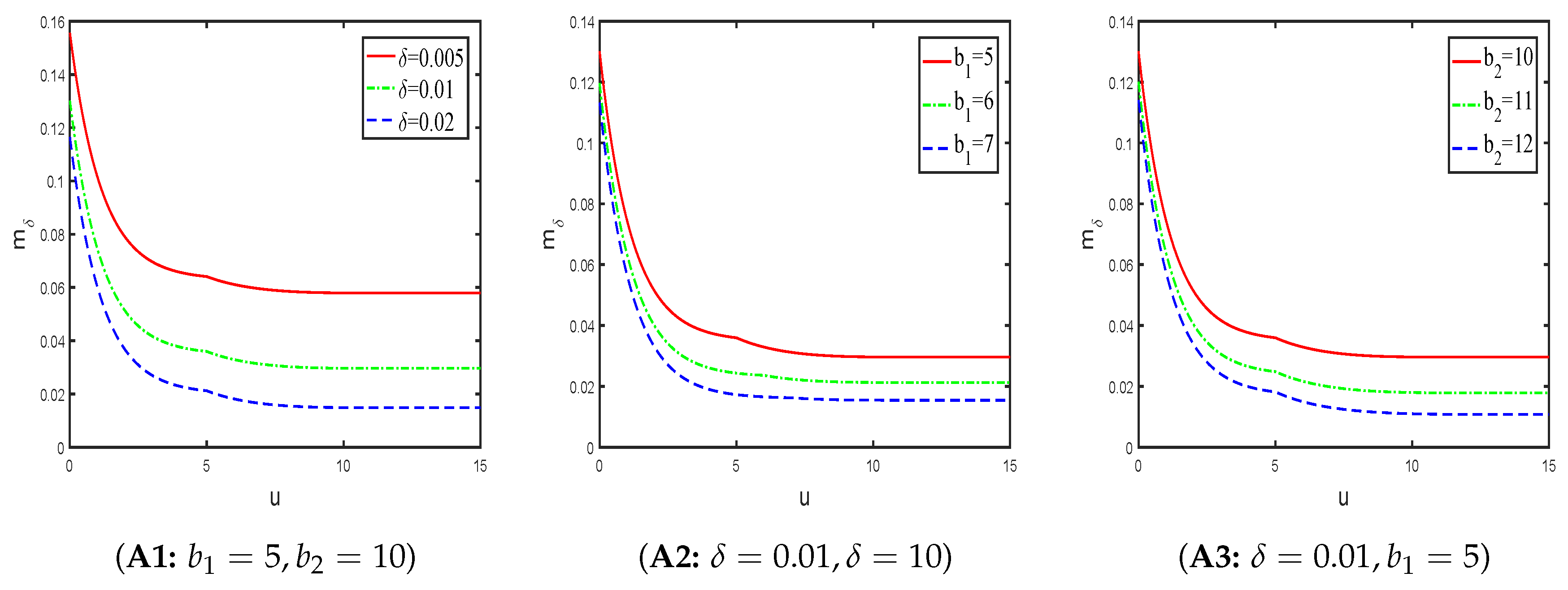
It should be noted that the above formula indicates that we can give explicit expressions under certain circumstances. In order to fully show the influence of parameters change on the function, we will give the numerical simulation as a whole, which is independent of the above explicit expressions. In fact, now the Gerber-Shiu function becomes the Laplace transformation of ruin time. The influence of interest force $\delta$, injection line $b_1$ and dividend payment line $b_2$ on Laplace transformation of ruin time is considered separately.

As can be seen from the three graphs in Figure 2, the Laplace transformation of ruin time is a decreasing function of initial reserve u, which is inconsistent with the conclusion of traditional classical model. This means that the higher initial reserve u is, the smaller the Laplace transformation of ruin time is. The reason is that $e^{-\delta {\tau }_{b_1}^{b_2}}$ is a decreasing function of ruin time ${\tau }_{b_1}^{b_2}$. Increased initial reserve u means greater ruin time ${\tau }_{b_1}^{b_2}$, which in turn leads to smaller function $e^{-\delta {\tau }_{b_1}^{b_2}}$. In addition, if the initial reserve u is fixed, the Laplace transformation of ruin time is a decreasing function for parameters $\delta$, $b_1$ and $b_2$, respectively. Take $b_2$ as an example, larger $b_2$ means larger ${\tau }_{b_1}^{b_2}$, which in turn leads to smaller function $e^{-\delta {\tau }_{b_1}^{b_2}}$. The same conclusion appears in $b_1$ and $\delta$, and we are not explain it one more time.

Example 2.

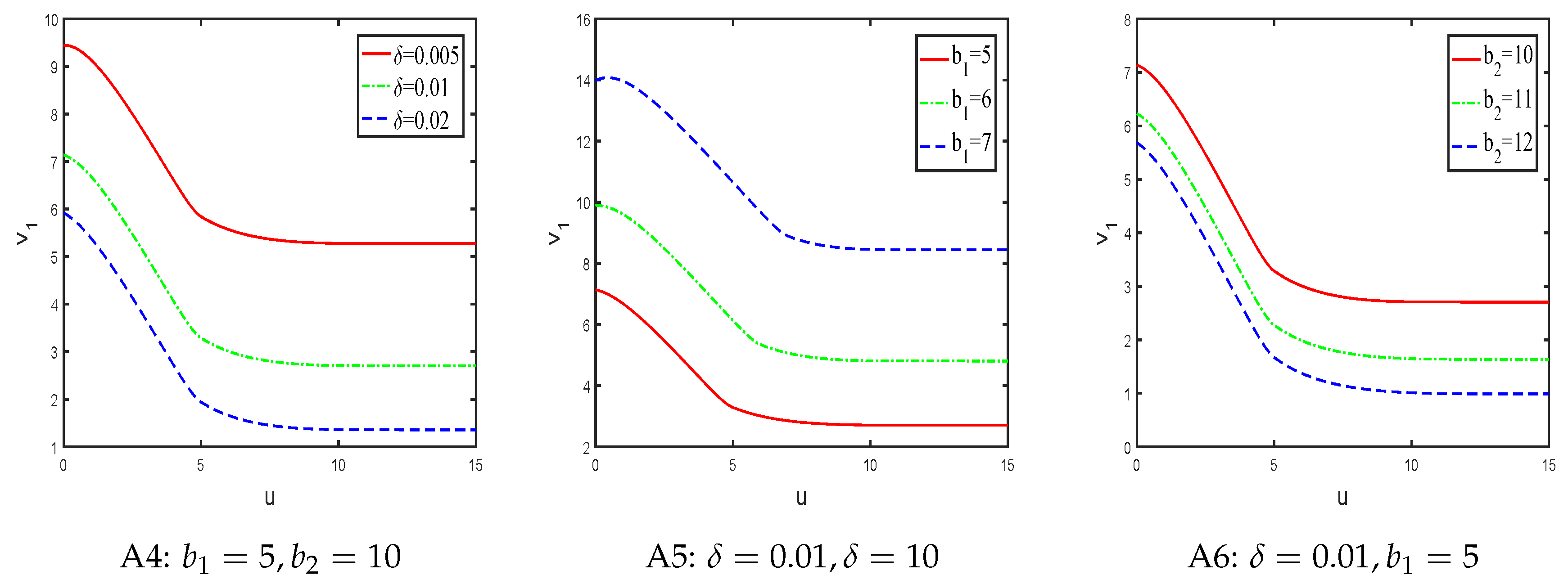
Suppose the observational time interval, claim arrival time and claim amount are exponentially distributed with parameters $\gamma =5$, $\lambda =1$ and $\beta =1$, respectively. The net premium rate $c=2$, Now the influence of interest force δ, injection line $b_1$ and dividend payment line $b_2$ on expected discount capital injection until ruin is considered separately.

As can be seen from the three graphs in Figure 3, the expected discount capital injection until ruin is a deceasing function of initial reserve u. In addition, if the initial reserve u is fixed, the expected discount capital injection until ruin is a deceasing function for parameters $\delta$ and $b_2$, respectively, and an increasing function of parameters $b_1$.

Example 3.

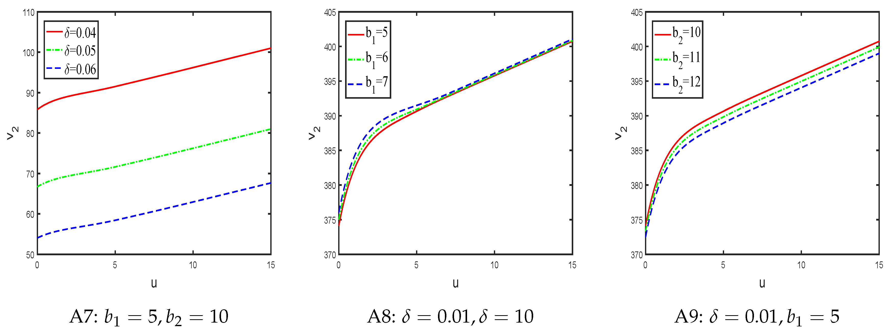
Suppose the observational time interval, claim arrival time and claim amount are exponentially distributed with parameters $\gamma =5$, $\lambda =1$ and $\beta =1$, respectively. The net premium rate $c=2$. Now the influence of interest force δ, injection line $b_1$ and dividend payment line $b_2$ on expected discount capital injection until ruin is considered separately.

As can be seen from the three graphs in Figure 4, expected discount dividend function until ruin is an increasing function of initial reserve u. In addition, if the initial reserve u is fixed, expected discount dividend function until ruin is a deceasing function for parameters $\delta$ and $b_2$, respectively, and an increasing function of parameters $b_1$.

6. Conclusions

In this paper, on the basis of the classical risk model, we assume that the reserve level of an insurance company can only be observed at discrete time points, then a new risk model is proposed by introducing periodic capital injection strategy and barrier dividend strategy into the classical risk model under the assumption that the observation interval is subject to exponential distribution. This new risk model is of great practical significance since it is much closer to the actual operate model of an insurance company. On the assumption that the claim amount is subject to exponential distribution, the explicit expression of the Gerber-Shiu function is derived by means of the integral and differential method, and the explicit expression of the expected discount capital injection function and the expected discount dividend function is further derived. Finally, some numerical examples are given to further analyze the influence of relevant parameters on actuarial quantity of the risk model. These results will provide reference for risk management of insurance companies.

However, it is worth noting that the level line of capital injection and dividend in this model are assumed in advance, not necessarily the optimal level line of capital injection and dividend. So in the later stage, we can also focus on the selection of the optimal level of capital injection and dividend. In addition, we can also consider that the observation interval obeys Erlang(n) distribution.

References

1. Chi, Y.C.; Lin, X.S. On the threshold dividend strategy for a generalized jump-diffusion risk model. Insur. Math. Econ. 2011, 48, 326–337. [Google Scholar] [CrossRef]
2. Yin, C.C.; Wen, Y.Z.; Zhao, Y.X. On the optimal dividend problem for a spectrally positive Lévy process. ASTIN Bull. 2014, 44, 635–651. [Google Scholar] [CrossRef] [Green Version]
3. Li, S.M.; Lu, Y. On the time and the number of claims when the surplus drops below a certain level. Scand. Actuar. J. 2016, 2016, 420–445. [Google Scholar] [CrossRef]
4. Zeng, Y.; Li, D.P.; Chen, Z.; Yang, Z. Ambiguity aversion and optimal derivative-based pension investment with stochastic income and volatility. J. Econ. Dyn. Control 2018, 88, 70–103. [Google Scholar] [CrossRef] [Green Version]
5. Zeng, Y.; Li, D.P.; Gu, A.L. Robust equilibrium reinsurance-investment strategy for a mean-variance insurer in a model with jumps. Insur. Math. Econ. 2016, 66, 138–152. [Google Scholar] [CrossRef]
6. Yu, W.G.; Huang, Y.J.; Cui, C.R. The absolute ruin insurance risk model with a threshold dividend strategy. Symmetry 2018, 10, 377. [Google Scholar] [CrossRef] [Green Version]
7. Zhou, J.M.; Mo, X.Y.; Ou, H.; Yang, X.Q. Expected present value of total dividends in the compound binomial model with delayed claims and random income. Acta Math. Sci. 2013, 33, 1639–1651. [Google Scholar] [CrossRef]
8. Yu, W.G. Randomized dividends in a discrete insurance risk model with stochastic premium income. Math. Probl. Eng. 2013, 2013, 579534. [Google Scholar] [CrossRef]
9. Zhang, Z.M.; Yong, Y.D.; Yu, W.G. Valuing equity-linked death benefits in general exponential Lévy models. J. Comput. Appl. Math. 2020. [Google Scholar] [CrossRef]
10. Zhou, M.; Yuen, K.C.; Yin, C.C. Optimal investment and premium control in a nonlinear diffusion model. Acta Math. Appl. Sin.-E 2017, 33, 945–958. [Google Scholar] [CrossRef] [Green Version]
11. Yu, W.G.; Yong, Y.D.; Guan, G.F.; Huang, Y.J.; Su, W.; Cui, C.R. Valuing guaranteed minimum death benefits by cosine series expansion. Mathematics 2019, 7, 835. [Google Scholar] [CrossRef] [Green Version]
12. Xu, L.; Yao, D.J.; Cheng, G.P. Optimal investment and dividend for an insurer under a Markov regime switching market with high gain tax. J. Ind. Manag. Optim. 2020, 16, 325–356. [Google Scholar] [CrossRef] [Green Version]
13. Liu, J.; Zhao, Z.Q.; Yu, W.G.; Zhang, T.Q. Triple solutions for a damped impulsive differential equation. Adv. Differ. Equ. 2019. [Google Scholar] [CrossRef] [Green Version]
14. Peng, J.Y.; Wang, D.C. Uniform asymptotics for ruin probabilities in a dependent renewal risk model with stochastic return on investments. Stochastics 2018, 90, 432–471. [Google Scholar] [CrossRef]
15. Wang, Y.Y.; Yu, W.G.; Huang, Y.J.; Yu, X.L.; Fan, H.L. Estimating the expected discounted penalty function in a compound Poisson insurance risk model with mixed premium income. Mathematics 2019, 7, 305. [Google Scholar] [CrossRef] [Green Version]
16. Asmussen, S.; Albrecher, H. Ruin Probabilities; World Scientific Publishing: Singapore, 2010. [Google Scholar]
17. Albrecher, H.; Cheung, E.C.K.; Thonhauser, S. Randomized observation periods for the compound Poisson risk model: Dividends. ASTIN Bull. 2011, 41, 645–672. [Google Scholar]
18. Albrecher, H.; Cheung, E.C.K.; Thonhauser, S. Randomized observation periods for the compound Poisson risk model: The discounted penalty function. Scand. Actuar. J. 2013, 2013, 424–452. [Google Scholar] [CrossRef]
19. Choi, M.C.H.; Cheung, E.C.K. On the expected discounted dividends in the Cramer-Lundberg risk model with more frequent ruin monitoring than dividend decisions. Insur. Math. Econ. 2014, 59, 121–132. [Google Scholar] [CrossRef] [Green Version]
20. Avanzi, B.; Cheung, E.C.K.; Wong, B.; Woo, J.K. On a periodic dividend barrier strategy in the dual model with continuous monitoring of solvency. Insur. Math. Econ. 2013, 52, 98–113. [Google Scholar] [CrossRef] [Green Version]
21. Zhang, Z.M.; Cheung, E.C.K.; Yang, H.L. Lévy insurance risk process with Poissonian taxation. Scand. Actuar. J. 2017, 2017, 51–87. [Google Scholar] [CrossRef] [Green Version]
22. Zhang, Z.M.; Cheung, E.C.K.; Yang, H.L. On the compound Poisson risk model with periodic capital injections. ASTIN Bull. 2018, 48, 435–477. [Google Scholar] [CrossRef] [Green Version]
23. Cheung, E.C.K.; Zhang, Z.M. Periodic threshold type dividend strategy in the compound Poisson risk model. Scand. Actuar. J. 2019, 2019, 1–31. [Google Scholar] [CrossRef]
24. Peng, X.H.; Su, W.; Zhang, Z.M. On a perturbed compound Poisson risk model under a periodic threshold-type dividend strategy. J. Ind. Manag. Optim. 2019. [Google Scholar] [CrossRef]
25. Yang, L.; Deng, G.H. A perturbed risk model with constant interest and periodic barrier dividend strategy. Commun. Stat.-Simul. C 2019. [Google Scholar] [CrossRef]
26. Zhang, Z.M.; Liu, C.L. Moments of discounted dividend payments in a risk model with randomized dividend-decision times. Front. Math. China 2017, 12, 493–513. [Google Scholar] [CrossRef]
27. Zhang, Z.M. On a risk model with randomized dividend-decision times. J. Ind. Manag. Optim. 2013, 10, 1041–1058. [Google Scholar] [CrossRef]
28. Zhang, Z.M.; Han, X. The compound Poisson risk model under a mixed dividend strategy. Appl. Math. Comput. 2017, 315, 1–12. [Google Scholar] [CrossRef]
29. Zhao, Y.X.; Chen, P.; Yang, H.L. Optimal periodic dividend and capital injection problem for spectrally positive Lévy processes. Insur. Math. Econ. 2017, 74, 135–146. [Google Scholar] [CrossRef] [Green Version]
30. Pérez, J.L.; Yamazaki, K. On the optimality of periodic barrier strategies for a spectrally positive Lévy process. Insur. Math. Econ. 2017, 77, 1–13. [Google Scholar] [CrossRef] [Green Version]
31. Noba, K.; Pérez, J.L.; Yamazaki, K.; Yano, K. On optimal periodic dividend and capital injection strategies for spectrally negative Lévy models. J. Appl. Probabil. 2018, 55, 1272–1286. [Google Scholar] [CrossRef] [Green Version]
32. Dong, H.; Zhou, X.W. On a spectrally negative Lévy risk process with periodic dividends and capital injections. Stat. Probabil. Lett. 2019, 155. [Google Scholar] [CrossRef]
33. Xu, R.; Woo, J.K.; Han, X.X.; Yang, H.L. A plan of capital injections based on the claims frequency. Ann. Actuar. Sci. 2018, 12, 296–325. [Google Scholar] [CrossRef]
34. Zhang, Z.M.; Yang, Y.; Liu, C.L. On a perturbed compound Poissom model with varying premium rates. J. Ind. Manag. Optim. 2017, 13, 721–736. [Google Scholar]
35. Liu, J.; Yu, W.G. Two solutions to superlinear Hamiltonian systems with impulsive effects. Appl. Math. Lett. 2020. [Google Scholar] [CrossRef]
36. Zhang, Z.M.; Cheung, E.C.K. The Markov additive risk process under an Erlangized barrier dividend strategy. Methodol. Comput. Appl. 2016, 18, 275–306. [Google Scholar] [CrossRef] [Green Version]
37. Yu, W.G.; Wang, F.; Huang, Y.J.; Liu, H.D. Social optimal mean field control problem for population growth model. Asian J. Control 2019, 1–8. [Google Scholar] [CrossRef]
38. Liu, C.L.; Zhang, Z.M. On a discrete risk model with delayed claims and a randomized dividend strategy. Adv. Differ. Equ.-Ny. 2015, 2015, 284. [Google Scholar] [CrossRef] [Green Version]
39. Gerber, H.U.; Shiu, E.S.W. On the time value of ruin. N. Am. Actuar. J. 1998, 2, 48–78. [Google Scholar] [CrossRef]
40. Lin, X.S.; Willmot, G.E.; Drekic, S. The classical risk model with a constant dividend barrier: Analysis of the Gerber-Shiu discounted penalty function. Insur. Math. Econ. 2003, 33, 551–566. [Google Scholar]
41. Huang, Y.J.; Yu, W.G. The Gerber-Shiu discounted penalty function of Sparre Andersen risk model with a constant dividend barrier. Math. Probl. Eng. 2014, 2014, 450149. [Google Scholar] [CrossRef] [Green Version]
42. Ruan, J.C.; Yu, W.G.; Song, K.; Sun, Y.H.; Huang, Y.J.; Yu, X.L. A note on a generalized Gerber-Shiu function in a compound Poisson risk model. Mathematics 2019, 7, 891. [Google Scholar] [CrossRef] [Green Version]
43. Li, S.M.; Lu, Y.; Sendova, K.P. The expected discounted penalty function: From infinite time to finite time. Scand. Actuar. J. 2019, 2019, 336–354. [Google Scholar] [CrossRef]
44. Wang, Y.Y.; Yu, W.G.; Huang, Y.J. Estimating the Gerber-Shiu function in a compound Poisson risk model with stochastic premium income. Discret. Dyn. Nat. Soc. 2019, 2019, 5071268. [Google Scholar] [CrossRef]
45. Yang, Y.; Su, W.; Zhang, Z.M. Estimating the discounted density of the deficit at ruin by Fourier cosine series expansion. Stat. Probabil. Lett. 2019, 146, 147–155. [Google Scholar] [CrossRef]
46. Yu, W.G. Some results on absolute ruin in the perturbed insurance risk model with investment and debit interests. Econ. Model. 2013, 31, 625–634. [Google Scholar] [CrossRef]
47. Yu, W.G. On the expected discounted penalty function for a Markov regime switching risk model with stochastic premium income. Discret. Dyn. Nat. Soc. 2013, 2013, 320146. [Google Scholar] [CrossRef]
48. Yuen, K.C.; Wang, G.J.; Li, W.K. The Gerber-Shiu expected discounted penalty function for risk processes with interest and a constant dividend barrier. Insur. Math. Econ. 2007, 40, 104–112. [Google Scholar] [CrossRef]
49. Huang, Y.J.; Yu, W.G.; Pan, Y.; Cui, C.R. Estimating the Gerber-Shiu expected discounted penalty function for Lévy risk model. Discret. Dyn. Nat. Soc. 2019, 2019, 3607201. [Google Scholar] [CrossRef] [Green Version]
50. Xie, J.H.; Zou, W. On the expected discounted penalty function for a risk model with dependence under a multi-layer dividend strategy. Commun. Stat.-Theory Methods 2016, 46, 1898–1915. [Google Scholar] [CrossRef]
Figure 1. A sample path of U b 1 b 2 ( t ) .
Mathematics 08 00511 g001
Figure 2. The Laplace transformation of the ruin time.
Mathematics 08 00511 g002
Figure 3. Expected discount capital injection until ruin.
Mathematics 08 00511 g003
Figure 4. Expected discount dividend function until ruin.
Mathematics 08 00511 g004