Generalized Fuzzy Graph Connectivity Parameters with Application to Human Trafficking

Abstract

Graph models are fundamental in network theory. But normalization of weights are necessary to deal with large size networks like internet. Most of the research works available in the literature have been restricted to an algorithmic perspective alone. Not much have been studied theoretically on connectivity of normalized networks. Fuzzy graph theory answers to most of the problems in this area. Although the concept of connectivity in fuzzy graphs has been widely studied, one cannot find proper generalizations of connectivity parameters of unweighted graphs. Generalizations for some of the existing vertex and edge connectivity parameters in graphs are attempted in this article. New parameters are compared with the old ones and generalized values are calculated for some of the major classes like cycles and trees in fuzzy graphs. The existence of super fuzzy graphs with higher connectivity values are established for both old and new parameters. The new edge connectivity values for some wider classes of fuzzy graphs are also obtained. The generalizations bring substantial improvements in fuzzy graph clustering techniques and allow a smooth theoretical alignment. Apart from these, a new class of fuzzy graphs called generalized t-connected fuzzy graphs are studied. An algorithm for clustering the vertices of a fuzzy graph and an application related to human trafficking are also proposed.

1. Introduction

The 20th century witnessed several major revolutions in mathematics. The invention of fuzzy logic by Zadeh [1] in 1965 is a remarkable one with several implications and amazing consequences. Zadeh’s logic has been applied in different fields including knowledge based systems, control theory and manufacturing. Several new fields in mathematics also emerged as a consequence. Rosenfeld [2] presented a new version of graph theory, called fuzzy graph theory in $1975.$ A fuzzy graph represents a capacity-normalized network having different degrees of vagueness associated with its vertices and links. This new theory is helpful in modeling large inter-connection networks like internet and power grids.

Fuzzy graph theory has grown as an intense area of research today. The most important and applicable concept in this area is that of connectivity. There are several classical problems like maximum band-width problems, bottleneck problems, quality of service problems, and so forth., in network theory, applying different connectivity parameters. A study of connectivity of fuzzy graphs can be found in Reference [2,3,4]. It can be observed that none of these works contain proper generalizations of connectivity parameters of graphs. This is the motivation behind this paper. The authors generalize the basic graph concepts inline with the classical ones, and make a comparison. The definitions of fuzzy vertex connectivity and fuzzy edge connectivity given in Reference [3] were based on strong edges of fuzzy graphs and hence were not direct of generalizations of cut vertices and bridges in graph theory. In this paper, we rectify this problem by providing new definitions for vertex connectivity and edge connectivity in fuzzy graphs.

The major contribution of this paper include the existence theorems for fuzzy graphs with arbitrary connectivity values and computation of fuzzy edge connectivity parameters for certain special sub-categories of fuzzy graphs, which include saturated and $\beta$-saturated cycles, and complements of fuzzy graphs. The values of the new parameters are also calculated for fuzzy cycles, fuzzy trees and complete fuzzy graphs. Some existence theorems and constructions in the generalized case are also provided. The existence of a super fuzzy graph having more fuzzy edge connectivity than that of a given fuzzy graph and the construction of a t-edge connected complete fuzzy graph are provided in the beginning. An example of clustering in fuzzy graphs exhibiting the superiority of the new parameters over the existing ones is provided towards the end.

The first paper in fuzzy graph theory by Rosenfeld [2] addressed the problem of clustering using the concept of vertex connectivity. One can find fuzzified versions of most of the concepts in graph theory, in Reference [2]. Cut vertices, bridges, blocks, and so forth are generalized. Several major characterizations are provided in this paper. An independent definition of fuzzy graphs were given by Yeh and Bang in Reference [4] simultaneously. They studied vertex connectivity and edge connectivity of fuzzy graphs and used them in fuzzy graph clustering. Bhattacharya et al. [5,6] studied this further and provided several algorithms related to connectivity. Bhutani et al. introduced the concept of strong edge in Reference [7]. They also investigated automorphism of fuzzy graphs [8], fuzzy end vertices [9] and geodesics in fuzzy graphs [10]. Sunitha and Vijayakumar [11,12] came up with several characterizations of fuzzy trees and blocks. They also studied complement of fuzzy graphs [13] and several matrices in fuzzy graphs [11]. In $2009,$ Mathew and Sunitha [14] identified different types of edges in fuzzy graphs and provided an algorithm for the same. They characterized many fuzzy graph structures like fuzzy trees, blocks and complete fuzzy graphs in an effective way using this identification. Fuzzy vertex connectivity and fuzzy edge connectivity were introduced in $2010,$ by the authors of Reference [3]. They were generalizations of Yeh and Bang’s connectivity parameters. In $2013,$ Mathew and Sunitha introduced the cyclic connectivity in fuzzy graphs [15]. In $2015,$ Anjali et al. studied blocks in fuzzy graphs in detail. This work can be found in References [16,17,18]. Also, related works can be seen in [19,20].

A large number of variants of fuzzy graphs like, bipolar fuzzy graphs [21], interval-valued fuzzy line graphs [22], strong intuitionistic fuzzy graphs [23], and incidence fuzzy graphs [24] have been recently introduced in the literature. Connectivity concepts in fuzzy incidence graphs were studied by Mordeson, et al. [24,25,26,27,28]. Recently, Binu et al. introduced several indices like Wiener index [29], connectivity index [30] and cyclic connectivity index [31] and applied them in different types of interconnection networks. This work is a continuation of the work in Reference [3].

Section 2 contains preliminaries and Section 3, some results on fuzzy vertex and edge connectivity. Fuzzy edge connectivity of saturated fuzzy cycles and complements of cycles are some of the topics tackled in this section. Section 4 presents generalized connectivity parameters and find their relationships with the existing ones. Section 5 gives an algorithm for fuzzy graph clustering using the new parameters and Section 6 contains an application related to human trafficking.

2. Preliminaries

Let X be a set. A fuzzy subset $\sigma$ on X is a function $\sigma :X\to [0,1]$ [1]. Most of the fundamental definitions of fuzzy graph theory are given by Rosenfeld [2] and Yeh and Bang [4]. A fuzzy graph $G=(\sigma ,\mu )$ is a pair where $\sigma$ is a fuzzy subset of a set S and $\mu$ is a fuzzy subset of $S\times S$ such that $\mu (u,v)\le \sigma \left(u\right)\wedge \sigma \left(v\right)$ [2]. Since we consider only undirected fuzzy graphs we denote the edge $(u,v)$ or $(v,u)$ by $uv.$ A fuzzy graph $H=(\tau ,\nu )$ is called a partial fuzzy subgraph of G if $\tau \left(u\right)\le \sigma \left(u\right)$ for every $u\in {\tau }^{*}$ and $\nu \left(uv\right)\le \mu \left(uv\right)$ for every $\left(uv\right)\in {\nu }^{*}.$ A partial subgraph with $\tau \left(u\right)\le \sigma \left(u\right),$ $v\in {\tau }^{*}$ and $\nu \left(uv\right)=\mu \left(uv\right)$ for all $uv\in v^{*},$ is called a fuzzy subgraph of G [2]. A path P of length n is a sequence of distinct vertices $u_0,u_1,u_2,\cdots ,u_n$ with $\mu \left(u_{i-1}{u}_i\right)>0$ for $i=1,2,\cdots ,n.$ The strength of that path is the membership value of a weakest edge in $P.$ A path is called a cycle if $u_0=u_n,$ and is called a fuzzy cycle if it contains more than one weakest edge [4]. The strength of connectedness between some pair of vertices x and y is the maximum of strengths of all paths between that pairs and is denoted by $CON{N}_G(x,y).$ If the strength of a path P from x to y is equal to $CON{N}_G(x,y),$ then P is called a strongest $x-y$ path. If $CON{N}_G(x,y)>0$ for any $x,y\in {\sigma }^{*},$ then G is called a connected fuzzy graph [32]. If $\mu \left(xy\right)>CON{N}_{G-\left\{xy\right\}}(x,y)$ then $xy$ is called $\alpha -$strong and if $\mu \left(xy\right)=CON{N}_{G-\left\{xy\right\}}(x,y),$ then $xy$ is called $\beta -$strong. Otherwise it is a $\delta -$edge. $\alpha -$strong and $\beta -$strong edges are called strong edges and a path is called a strong path if all of its edges are strong [14].

An edge $xy\in {\mu }^{*}$ is called a fuzzy bridge if its removal reduces the strength of connectedness between some pair of vertices in G [2]. Similarly a vertex $v\in {\sigma }^{*}$ is said to be a fuzzy cut vertex of G if its removal decreases the strength of connectedness between some pair of vertices. A connected fuzzy graph $G=(\sigma ,\mu )$ is a fuzzy tree if it has a fuzzy spanning subgraph $F=(\sigma ,\nu )$ which is a tree, where for all edges $xy$ not in $F,$ there exists a path from x to y in $F,$ whose strength is more than $\mu \left(xy\right)$ [2]. A complete fuzzy graph $G=(\sigma ,\mu )$ is a fuzzy graph with the property $\mu \left(xy\right)=\sigma \left(x\right)\wedge \sigma \left(y\right)$ for all $x,y\in {\sigma }^{*}.$ G is said to be $\alpha -$saturated, if at least one $\alpha -$strong edge is incident at every vertex $v\in {\sigma }^{*},$ and is called $\beta -$saturated, if at least one $\beta -$strong edge is incident at every vertex. G is called saturated if it is both $\alpha$ and $\beta -$saturated [33].

A disconnection of a fuzzy graph $G=(\sigma ,\mu )$ is a vertex set $D\subset {\sigma }^{*}$ whose removal results in a disconnected or a single vertex fuzzy graph. The weight of D is defined to be ${\sum }_{v\in D}\wedge \left\{\mu \left(vu\right)\right|\mu \left(vu\right)\ne 0\}.$ The vertex connectivity of a fuzzy graph G denoted by $\Omega \left(G\right),$ is defined to be the minimum weight of a disconnection in G [4]. Let $G=(\sigma ,\mu )$ be a connected fuzzy graph. A set of vertices $X=\left\{v_1,v_2,\dots ,v_m\right\}\subset {\sigma }^{*}$ is said to be a fuzzy vertex cut or fuzzy node cut (FNC) if either, $CON{N}_{G-X}(x,y)<CON{N}_G(x,y)$ for some pair of vertices $x,y\in {\sigma }^{*}$ such that both $x,y\ne v_i$ for $i=1,2,\dots ,m$ or $G-X$ is trivial. Let X be a fuzzy vertex cut in $G.$ The strong weight of $X,$ denoted by $s\left(X\right)$ is defined as $s\left(X\right)={\sum }_{x\in X}\mu \left(xy\right),$$\mu \left(xy\right)$ is the minimum of the weights of strong edges incident at $x.$ The fuzzy vertex connectivity of a connected fuzzy graph G is defined as the minimum strong weight of fuzzy vertex cuts of $G.$ It is denoted by $\kappa \left(G\right)$ [3]. Let G be a fuzzy graph and $\left\{V_1,V_2\right\}$ be a partition of its vertex set. The set of edges joining vertices of $V_1$ and vertices of $V_2$ is called a cut-set of $G,$ denoted by $\left(V_1,V_2\right)$ relative to the partition $\left\{V_1,V_2\right\}.$ The weight of the cut-set $\left(V_1,V_2\right)$ is defined as ${\sum }_{u\in V_1,v\in V_2}\mu \left(uv\right).$ Let G be a fuzzy graph. The edge connectivity of G denoted by $\lambda \left(G\right)$ is defined to be the minimum weight of cut-sets of G [4]. Let $G=(\sigma ,\mu )$ be a fuzzy graph, a set of strong edges $E=\{e_1,e_2,\cdots ,e_n\}$ with $e_i=u_i{v}_i,i=1,2,\cdots ,n$ is said to be a fuzzy edge cut or fuzzy arc cut (FAC) if either $CON{N}_{G-E}(x,y)<CON{N}_G(x,y)$ for some pair of vertices $x,y\in {\sigma }^{*}$ with at least one of x or y different from both $u_i$ and $v_i,$$i=1,2,\cdots ,n,$ or $G-E$ is disconnected. The strong weight of a fuzzy edge cut E is defined as $s^{\prime }\left(E\right)=$ ${\sum }_{e_i\in E}\mu \left(e_i\right).$ The fuzzy edge connectivity ${\kappa }^{\prime }\left(G\right)$ of a connected fuzzy graph G is defined to be the minimum strong weight of fuzzy edge cuts of $G.$ Let G be a connected fuzzy graph and $t\in (0,\infty ),$ G is called t-connected if $\kappa \left(G\right)\ge t$ and G is called t-edge connected if ${\kappa }^{\prime }\left(G\right)\ge t$ [3]. More basic definitions and results can be seen in References [24,25].

3. Fuzzy Vertex and Edge Connectivity

In this section, fuzzy vertex connectivity and fuzzy edge connectivity are studied. They were introduced in Reference [3]. Mainly cycles and their complements are discussed.

Theorem 1.

[34] Let $G=(\sigma ,\mu )$ be a fuzzy graph with $|{\sigma }^{*}|=n.$ If $H=(\sigma ,\nu )$ is a partial fuzzy subgraph of $G,$ then $\kappa \left(H\right)\le \kappa \left(G\right).$

Theorem 1 can be restated in fuzzy edge connectivity terms for a particular category of partial fuzzy subgraphs as follows.

Theorem 2.

Let $G=(\sigma ,\mu )$ be a fuzzy graph with $|{\sigma }^{*}|=n.$ If $H=(\sigma ,\nu )$ is a partial fuzzy subgraph having the same vertex set of $G,$ then ${\kappa }^{\prime }\left(H\right)\le {\kappa }^{\prime }\left(G\right).$

The proof of Theorem 2 is obvious and is omitted.

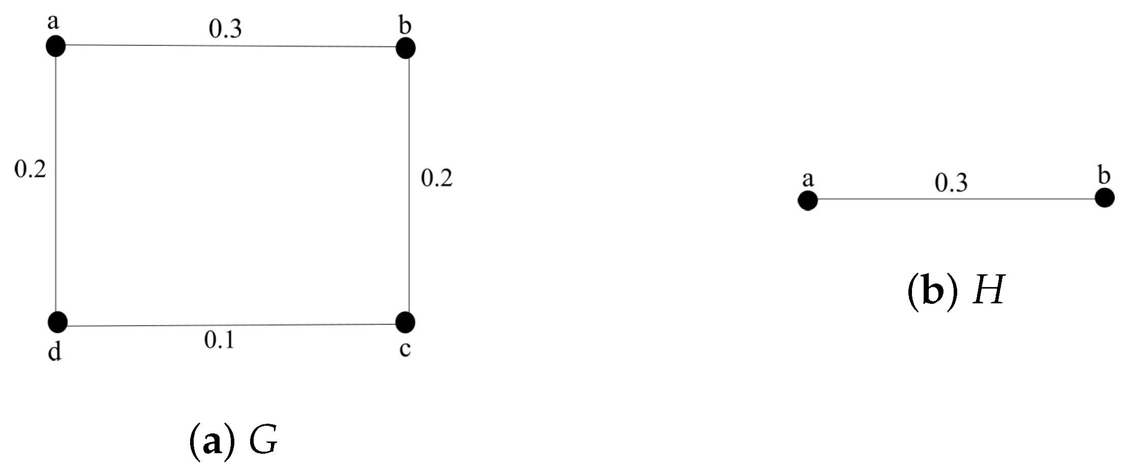
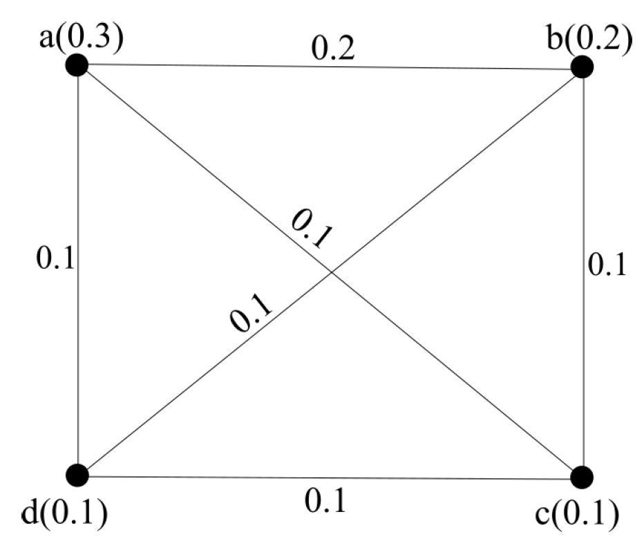
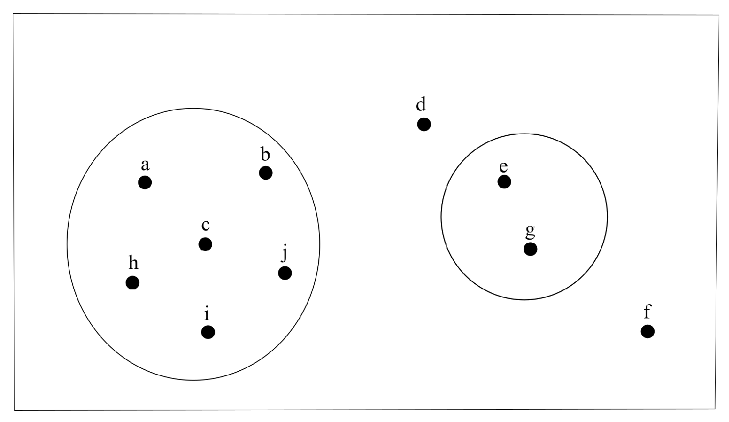
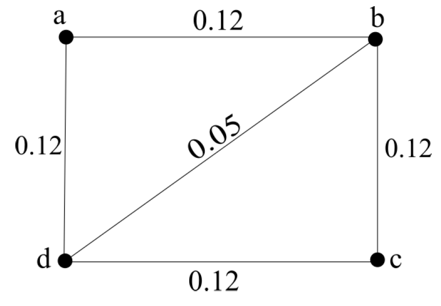
Note that in Theorem 2, the vertex set of H is the same as the vertex set of $G.$ This result is not true for every partial fuzzy subgraph of G, as seen from the fuzzy graph shown in Figure 1.

Figure 1. A fuzzy graph G having a subgraph H with ${\kappa }^{\prime }\left(H\right)>{\kappa }^{\prime }\left(G\right).$

In Figure 1, G is a fuzzy graph with ${\kappa }^{\prime }\left(G\right)=0.2.$ H is a partial fuzzy subgraph of G with ${\kappa }^{\prime }\left(H\right)=0.3.$

Note that the removal of an edge from a fuzzy graph never enhances its edge connectivity as seen from the following result.

Theorem 3.

For any fuzzy graph $G=(\sigma ,\mu ),$${\kappa }^{\prime }(G-e)\le {\kappa }^{\prime }\left(G\right),$ for every $e\in {\mu }^{*}.$

Proof of Theorem 3 follows from Theorem 2 and the fact that $G-e$ is a partial fuzzy subgraph of G on the same vertex set.

Next we study the existence of a super graph whose edge connectivity is greater than the edge connectivity of the original graph.

Theorem 4.

For any connected fuzzy graph with fuzzy edge connectivity ${\kappa }^{\prime }\left(G\right),$ there exists a connected super fuzzy graph $G^{\prime }$ of G with fuzzy edge connectivity ${\kappa }^{\prime }\left(G^{\prime }\right)>{\kappa }^{\prime }\left(G\right).$

Proof. 

Case 1. For any trivial fuzzy graph with ${\sigma }^{*}=\left\{u\right\},$${\kappa }^{\prime }\left(G\right)=0.$ Construct super fuzzy graph as $G^{\prime }=(\rho ,\nu )$ as ${\rho }^{*}={\sigma }^{*}\cup \left\{v\right\}$ and ${\nu }^{*}=\left\{uv\right\}.$ Define,

$$\rho \left(x\right)=\left\{\begin{array}{cc}\sigma \left(x\right)\hfill & ifx=u\hfill \\ 1\hfill & x=v\hfill \end{array}\right.$$

and $\nu \left(uv\right)=t,t\in (0,1].$ Clearly ${\kappa }^{\prime }\left(G^{\prime }\right)>{\kappa }^{\prime }\left(G\right).$

Case 2.

Let G be fuzzy graph with ${\sigma }^{*}=\{u,v\},$ and ${\mu }^{*}=\left\{uv\right\}.$ Thus in this case ${\kappa }^{\prime }\left(G\right)=\mu \left(uv\right)=t$(say). Construct a super graph $G^{\prime }=(\rho ,\nu )$ with ${\rho }^{*}={\sigma }^{*}\cup \left\{z\right\}$ and ${\nu }^{*}={\mu }^{*}\cup \{uz,vz\},$ with

$$\rho \left(x\right)=\left\{\begin{array}{cc}\sigma \left(x\right)\hfill & ifx\in {\sigma }^{*}\hfill \\ 1\hfill & ifx=z\hfill \end{array}\right.$$

and

$$\nu \left(xy\right)=\left\{\begin{array}{cc}\mu \left(xy\right)\hfill & ifxy=uv\hfill \\ s\hfill & ifxy=uzxy=vz,s\nleqq t.\hfill \end{array}\right.$$

If $s>t,$ Then, ${\kappa }^{\prime }\left(G^{\prime }\right)=s>t={\kappa }^{\prime }\left(G\right),$ else then, ${\kappa }^{\prime }\left(G^{\prime }\right)=2s>t={\kappa }^{\prime }\left(G\right).$

Case 3.

Let G be a complete fuzzy graph with n vertices say $\{v_1,v_2,\dots ,v_n\},n\ge 3.$ In this case ${\kappa }^{\prime }\left(G\right)=n*\wedge \{\sigma \left(x\right):x\in {\sigma }^{*}\}.$ Construct a super graph $G^{\prime }=(\rho ,\nu )$ as ${\rho }^{*}={\sigma }^{*}\cup \left\{z\right\}$ and ${\nu }^{*}={\mu }^{*}\cup \{v_{i}z:i=1,2,\dots n\}.$

$$\rho \left(x\right)=\left\{\begin{array}{cc}\sigma \left(x\right)\hfill & ifx\in {\sigma }^{*}\hfill \\ \wedge \{\sigma \left(x\right):x\in {\sigma }^{*}\}\hfill & ifx=z\hfill \end{array}\right.$$

and

$$\nu \left(xy\right)=\left\{\begin{array}{cc}\mu \left(xy\right)\hfill & ifxy\in {\mu }^{*}\hfill \\ \sigma \left(z\right)\hfill & Otherwise.\hfill \end{array}\right.$$

Thus $G^{\prime }$ becomes a CFG with $n+1$ vertices. So, ${\kappa }^{\prime }\left(G^{\prime }\right)=(n+1)*\wedge \{\sigma \left(x\right):x\in \rho *\}>n*\wedge \{\sigma \left(x\right):x\in {\sigma }^{*}\}={\kappa }^{\prime }\left(G\right).$

Case 4.

Let G is not a complete fuzzy graph with edge connectivity ${\kappa }^{\prime }\left(G\right).$

Let E be a minimum fuzzy edge cut of G and X be the collection of end vertices of $E.$ Then there exists a pair of vertices $u,v$ such that $CON{N}_{G-E}(u,v)<CON{N}_G(u,v),$ with at least one of u or v different from the end vertices of $E.$ If $uv$ is a $\delta -$edge, then there exist k internally disjoint strongest $u-v$ paths and $uv$ is the weakest edge of a $k-$cycle. Thus any minimum $u-v$ separating set has cardinality $k.$ Construct a super fuzzy graph $G^{\prime }=(\rho ,\nu )$ with ${\rho }^{*}={\sigma }^{*}\cup \left\{z\right\}$ and ${\nu }^{*}={\mu }^{*}\cup \{uz,vz\}.$

$$\rho \left(x\right)=\left\{\begin{array}{cc}\sigma \left(x\right)\hfill & ifx\in {\sigma }^{*}\hfill \\ 1\hfill & ifx=z\hfill \end{array}\right.$$

and

$$\nu \left(xy\right)=\left\{\begin{array}{cc}\mu \left(xy\right)\hfill & ifxy\in {\mu }^{*}\hfill \\ CON{N}_G(u,v)\hfill & ifx\notin Xory\notin X.\hfill \end{array}\right.$$

By construction, $u-v$ has $k+1$ internally disjoint strongest paths. Hence, minimum $u-v$ separating set $E^{\prime }$ has exactly $k+1$ edges. Moreover, $s^{\prime }\left(E^{\prime }\right)>s^{\prime }\left(E\right).$ If ${\kappa }^{\prime }\left(G^{\prime }\right)>{\kappa }^{\prime }\left(G\right)$ then $G^{\prime }$ becomes the super graph. But if ${\kappa }^{\prime }\left(G^{\prime }\right)={\kappa }^{\prime }\left(G\right),$ then let $E^{″}$ be a minimum fuzzy edge cut of $G^{\prime }.$ Then there exists a pair of vertices $u_1,v_1$ in $G^{\prime }$ such that $CON{N}_{G-E}(u_1,v_1)<CON{N}_G(u_1,v_1).$ If $u_1{v}_1$ is a $\delta -$edge or $u_1$ and $v_1$ are not adjacent, then the above procedure can be repeated. Suppose $G^{\prime }$ is disconnected. let Y be a minimum separating set in $G^{\prime },$ such that $G^{\prime }-E$ is disconnected. Construct $G^{″}=({\rho }^{\prime },{\nu }^{\prime }),$ with ${\rho }^{\prime *}={\rho }^{*}\cup \left\{z\right\}$ and ${\nu }^{\prime *}={\nu }^{*}\cup \{u_{2}z,v_{2}z\},$ where $u_2$ and $v_2$ are in different components with minimum strength of connectedness.

$${\rho }^{\prime }\left(x\right)=\left\{\begin{array}{cc}\sigma \left(x\right)\hfill & ifx\in {\rho }^{*}\hfill \\ 1\hfill & ifx=z\hfill \end{array}\right.$$

and

$${\nu }^{\prime }\left(xy\right)=\left\{\begin{array}{cc}\mu \left(xy\right)\hfill & ifxy\in {\nu }^{*}\hfill \\ CON{N}_G(u_2,v_2)\hfill & ifxy=u_{2}zorxy=v_{2}z.\hfill \end{array}\right.$$

Let $Y^{\prime }$ be a minimum $u_2-v_2$ strength reducing set and there exist $Y+1$ internally disjoint strongest $u_2-v_2$ paths in $G^{″}.$ Hence, $s^{\prime }\left(Y^{\prime }\right)>s^{\prime }\left(Y\right).$ If ${\kappa }^{\prime }\left(G^{″}\right)>{\kappa }^{\prime }\left(G^{\prime }\right)$ then choose super graph as $G^{″}.$ Suppose ${\kappa }^{\prime }\left(G^{″}\right)={\kappa }^{\prime }\left(G^{\prime }\right).$ Repeat the above procedure that have been already discussed. □

Now we study the existence of $t-$edge connected complete fuzzy graphs.

Theorem 5.

There exists a $t-$edge connected complete fuzzy graph for any $t\in {\mathrm{I}\mathrm{R}}^{+}.$

Proof. 

Let us first assume that $t\in (0,1].$ A $t-$connected complete fuzzy graph is simply $G=K_2$ with ${\sigma }^{*}=\{u,v\}$ and $\mu \left(uv\right)\ge t.$

Suppose $t\ge 1,$ let $t\in [n,n+1)$ for some $n\in \mathrm{I}\mathrm{N}.$ Construct a fuzzy graph G with at least $n+2$ vertices namely $v_1,v_2,\dots ,v_{n+2},\dots ,v_{n+k}.$ Let $\sigma \left(v_i\right)\ge \frac{t}{(n+k-1)}$ for $i=1,2,\dots ,,n+k,$ and $\mu \left(v_i{v}_j\right)=\sigma \left(v_i\right)\wedge \sigma \left(v_j\right)$ for $i\ne j.$ Then G is a CFG with $n+k$ vertices. Without loss of generality we can assume $v_1$ be the vertex of minimum degree. Thus by Theorem 4 in Reference [3], ${\kappa }^{\prime }\left(G\right)=(n+k-1)*\wedge \{\sigma \left(x\right):x\in {\sigma }^{*}\}.$ Hence, ${\kappa }^{\prime }\left(G\right)\ge (n+k)*\frac{t}{(n+k-1)}=t.$ Thus, G is a $t-$edge connected complete fuzzy graph. □

Theorem 6.

Let G be a $t-$connected fuzzy graph and let E be a minimum fuzzy edge cut of $G.$ Let $G^{\prime }$ be a fuzzy graph obtained by adding a new vertex z to G and joining z to the end vertices of $E.$ Let $\mu \left(v_{i}z\right)=\wedge \{\mu \left(v_{i}u\right):v_{i}u$ is a strong edge in $G\}.$ Then $G^{\prime }$ is $t-$edge connected.

Proof. 

Let $G=(\sigma ,\mu )$ be a $t-$edge connected fuzzy graph and E be a fuzzy edge cut with minimum strong weight and X be the set of end vertices of edges in $E.$ Let $G^{\prime }$ be the fuzzy graph obtained by adding a new vertex z to $G=(\rho ,\nu )$ and joining z to X and $\mu \left(v_{i}z\right)=\wedge \{\mu \left(v_{i}u\right):v_{i}u$ is a strong edge in $G\}.$ Let $E^{\prime }$ be the minimum fuzzy edge cut of $G^{\prime }.$

It is clear that the edges from ${\nu }^{*}\setminus {\mu }^{*}$ are all strong. Now let, $E^{\prime }$ contains edges from ${\nu }^{*}\setminus {\mu }^{*}.$ Then, removal of those edges from $E^{\prime }$ is a fuzzy edge cut for $G.$ Suppose $E^{\prime }$ contains no edges from ${\nu }^{*}\setminus {\mu }^{*}.$ Then $E^{\prime }$ itself is a fuzzy edge cut of $G.$ Thus, $s^{\prime }\left(E^{\prime }\right)>{\kappa }^{\prime }\left(G\right).$ In both cases, $s^{\prime }\left(E^{\prime }\right)>{\kappa }^{\prime }\left(G\right),$ Thus, ${\kappa }^{\prime }\left(G^{\prime }\right)\ge {\kappa }^{\prime }\left(G\right).$ Hence, $G^{\prime }$ is $t-$edge connected. □

Next we determine the fuzzy edge connectivity of $\beta -$saturated fuzzy cycles.

Theorem 7.

Let $G=(\sigma ,\mu )$ be a fuzzy cycle with $|{\sigma }^{*}|\ge 3.$ If G is $\beta -$saturated, then ${\kappa }^{\prime }\left(G\right)=2\mu \left(xy\right),$ where $xy$ is a weakest edge of $G.$

Proof. 

Let $G=(\sigma ,\mu )$ be a $\beta -$saturated fuzzy cycle with $|{\sigma }^{*}|\ge 3.$ Then every vertex is incident with at least one $\beta -$strong edge. The removal of an $\alpha -$strong edge (if exists) affects only the connectivity of its end vertices, where as the removal of a $\beta -$strong edge never affects the connectivity in $G.$ Thus the removal of a single edge does not affect the edge connectivity between any pair of vertices in $G.$ Also removing any two edges from G disconnects the graph. Thus any two edges form a fuzzy cut set of $G,$ of which one having any two $\beta -$strong edges will have the minimum size. Hence, ${\kappa }^{\prime }\left(G\right)=2\mu \left(xy\right).$ □

Next we determine the fuzzy edge connectivity of odd cycles which are $\alpha -$saturated.

Theorem 8.

Let $G=(\sigma ,\mu )$ be an odd fuzzy cycle with $|{\sigma }^{*}|\ge 3.$ If G is $\alpha -$saturated and e is a weakest edge of $G,$ then ${\kappa }^{\prime }\left(G\right)=\wedge \{m,2\mu \left(e\right)\}$ where $m=\wedge${$\mu \left(uv\right)$: either u or v is incident with $\alpha -$strong edges only}.

Proof. 

Let $G=(\sigma ,\mu )$ be an odd fuzzy cycle with $|{\sigma }^{*}|\ge 3.$ Let X be the collection of vertices in G which are incident with $\alpha -$strong edges alone no $\beta -$strong edges. Since G is $\alpha -$saturated, and is an odd cycle, $\left|X\right|\ne 0.$ Let $u\in X$ and $v\in {\sigma }^{*}$ be such that $uv\in {\mu }^{*}.$ Note that $uv$ is an $\alpha -$strong edge. Being a cycle, there exists $w\in {\sigma }^{*}$ such that $uw$ is $\alpha -$strong. Hence the path $wuv$ is a unique path in $G.$ Removal of $uv$ affects the connectivity between w and $v.$ Also any two $\beta -$strong edges in G form a fuzzy edge cut, of G and the result follows. □

Next we consider the case of even saturated fuzzy cycles.

Theorem 9.

Let $G=(\sigma ,\mu )$ be an even saturated fuzzy cycle with $|{\sigma }^{*}|\ge 3.$ Then ${\kappa }^{\prime }\left(G\right)=2\mu \left(xy\right),$ where $xy$ is a weakest edge of $G.$

Proof. 

Let $G=(\sigma ,\mu )$ be an even saturated fuzzy cycle with $|{\sigma }^{*}|\ge 3,$ then every vertex in G is adjacent to at least one $\beta$-strong edge. No single edge will form a fuzzy edge cut. Collection of any two edges will form a minimal FEC. Of which two edges with minimum weights constitute a minimum fuzzy edge cut. Hence ${\kappa }^{\prime }\left(G\right)=2\mu \left(xy\right).$ □

Theorem 10.

Let $G=(\sigma ,\mu )$ be a fuzzy cycle with $|{\sigma }^{*}|=n\ge 5$ and $\sigma \left(u\right)=t,$$t\in (0,1].$ Then fuzzy edge connectivity of $G^c=(\sigma ,\nu )$ is, ${\kappa }^{\prime }\left(G^c\right)=(n-3)t.$

Proof. 

Let $G=(\sigma ,\mu )$ be a fuzzy cycle with $|{\sigma }^{*}|=n\ge 5.$ Let $\sigma \left(u\right)=t,$$t\in (0,1].$ Being a fuzzy cycle, G contains only strong edges. Also, $CON{N}_{G^c}(x,y)=t,\forall x,y\in {\sigma }^{*}.$ Clearly $uv\in {\mu }^{*}$ becomes a $\delta -$edge in $G^c,$ and there are exactly $n-3$ strong edges incident at every vertex in $G^c.$ Thus the removal of a set S of exactly $n-3$ vertices from G results in the inequality $CON{N}_{G-S}(x,y)<CON{N}_G(x,y)\forall x,y\in {\sigma }^{*}.$ Clearly there exists a pair of vertices $u,v$ with $uv\in {\mu }^{*}$ such that $S\left(P\right)=t$ for every $u-v$ path in $G^c.$ Thus by definition ${\kappa }^{\prime }\left(G^c\right)=(n-3)t.$ □

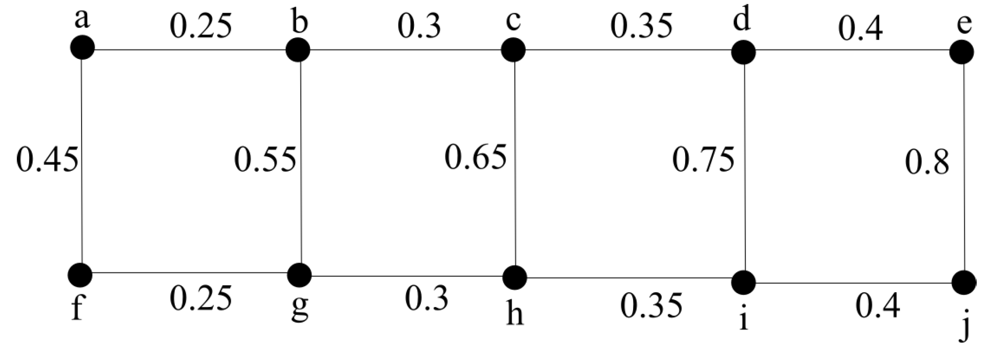
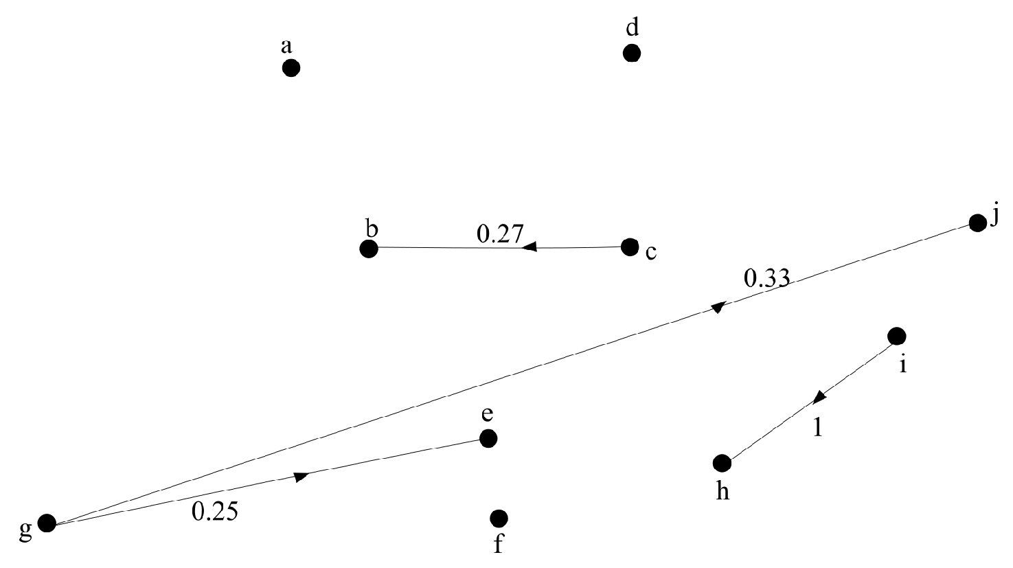
Example 1 illustrates Theorem 10.

Example 1.

Let G=$(\sigma ,\mu )$ be a fuzzy cycle given in Figure 2 with $V=\{a,b,c,d,e\}.$ Define fuzzy subsets σ of V and μ of $E=\{ab,bc,cd,de,ea\}$ as follows $\sigma \left(a\right)=0.5,\sigma \left(b\right)=0.3,\sigma \left(c\right)=0.2,\sigma \left(d\right)=0.4,$$\sigma \left(e\right)=0.5,$$\mu \left(ab\right)=0.3,\mu \left(bc\right)=0.1,\mu \left(cd\right)=0.1,\mu \left(de\right)=0.2$ and $\mu \left(ae\right)=0.2.$

Figure 2. Fuzzy graphs in Example 1.

Here G is a fuzzy cycle with value of t in Theorem 10 is $0.5.$ Now consider the fuzzy graph $G^c.$ Here, $\mu \left(cd\right)=0.4$ and $S\left(P\right)=0.5$ for all other paths from c to $d.$ There are exactly two strong paths from c to $d.$ Also, $ce$ and $ac$ are the strong edges incident at $c.$ Thus $S=\{ce,ac\}$ is a minimum fuzzy cut set for $G^c.$ So, ${\kappa }^{\prime }\left(G^c\right)=1.$

Theorem 11.

Let $G=(\sigma ,\mu )$ be a connected fuzzy graph with $|{\sigma }^{*}|=n.$ Then, ${\kappa }^{\prime }\left(G\right)\le {\kappa }^{\prime }\left(G^{\prime }\right)$ where $G^{\prime }=({\sigma }^{\prime },{\mu }^{\prime })$ is the complete fuzzy graph spanned by the vertex set of $G.$

Proof. 

Let $G=(\sigma ,\mu )$ be a connected fuzzy graph and $G^{\prime }=({\sigma }^{\prime },{\mu }^{\prime })$ be the complete fuzzy graph spanned by $\sigma .$ Let $v\in {\sigma }^{*}$ be a vertex of minimum degree in $G^{\prime }.$ Then ${\kappa }^{\prime }\left(G^{\prime }\right)=(n-1)\sigma \left(v\right).$ Let E denotes the set of edges incident at v in $G^{\prime }$ and $E^{\prime }$ that in $G.$ Then $E^{\prime }$ is a fuzzy edge cut in G and hence $s\left(E^{\prime }\right)\le s\left(E\right)={\kappa }^{\prime }\left(G^{\prime }\right).$ Therefore, conclusion holds for $G^{\prime }$ also. □

Theorem 12.

Let $G=(\sigma ,\mu )$ be a fuzzy tree and F be the corresponding MST of $G.$ Then ${\kappa }^{\prime }\left(G\right)={\kappa }^{\prime }\left(F\right).$

Proof follows from the fact that every strong edge of $G,$ belongs to $F.$

4. Generalized Fuzzy Vertex and Edge Connectivity

The concepts of fuzzy cut vertex and fuzzy bridge are generalized in this section. Generally in a fuzzy edge cut, we consider a set of strong edges $E=\{e_1,e_2,\cdots ,e_n\}$ where $e_i=u_i{v}_i,$$i=1,2,\dots ,n$ with either $CON{N}_{G-E}(x,y)<CON{N}_G(x,y)$ for some pair of vertices $x,y\in {\sigma }^{*}$ with at least one of x or y different from both $u_i$ and $v_i,$$i=1,2,\dots ,n,$ or $G-E$ is disconnected. But it can be seen that even non strong edges contribute towards the connectivity of fuzzy graphs significantly. Also, the condition that x and y should be different from the end vertices of edges in E disqualifies a fuzzy edge cut, being a generalization of classical cut set of edges. The definitions of fuzzy vertex connectivity and fuzzy edge connectivity are modified as in Definition 1.

Definition 1.

A set of vertices $X=\left\{v_1,v_2,\dots ,v_m\right\}\subset {\sigma }^{*}$ of a connected fuzzy graph $G=(\sigma ,\mu )$ is said to be ageneralized fuzzy vertex cut, if either, $CON{N}_{G-X}(x,y)<CON{N}_G(x,y)$ for some pair of vertices $x,y\in {\sigma }^{*}\setminus X$ or $G-X$ is trivial. Theweightof $X,$ denoted by $w_f\left(X\right)$ is defined as ${\displaystyle w_f\left(X\right)=\sum _{x\in X}\mu \left(xy\right),}$ where $\mu \left(xy\right)$ is the minimum of the weights of edges incident at $x.$ Thegeneralized fuzzy vertex connectivity of a connected fuzzy graph G is defined as the minimum weight of a generalized fuzzy vertex cut in $G.$ It is denoted by ${\kappa }_f\left(G\right).$

We call a generalized fuzzy vertex cut as a generalized fuzzy node cut occasionally, when we deal with networks and abbreviate it as a $g-FNC.$ Similar generalized definition for edges is as follows.

Definition 2.

Let $G=(\sigma ,\mu )$ be a fuzzy graph. A set of edges $E=\{e_1,e_2,\dots ,e_n\}$ is said to be ageneralized fuzzy edge cut(abbreviated as $g-FEC$) if either $CON{N}_{G-E}(x,y)<CON{N}_G(x,y)$ for some pair of vertices $x,y\in {\sigma }^{*}$ or $G-E$ is disconnected. 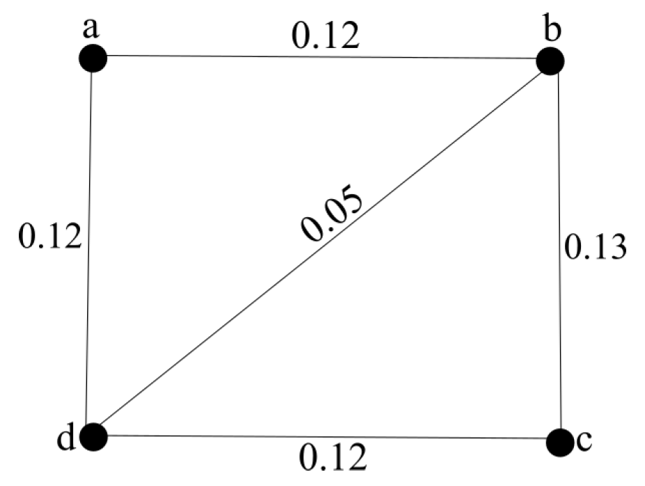Theweight of E is defined as $w_f^{\prime }\left(E\right)=$ ${\displaystyle \sum _{e_i\in E}\mu \left(e_i\right).}$ Thegeneralized fuzzy edge connectivity, ${\kappa }_f^{\prime }\left(G\right)$ of a connected fuzzy graph G is the minimum weight of a generalized fuzzy edge cut in $G.$

Define ${\kappa }_f\left(G\right)={\kappa }_f^{\prime }\left(G\right)=0$ for a disconnected or a trivial fuzzy graph. The fuzzy graph in Example 2 illustrates the above definitions.

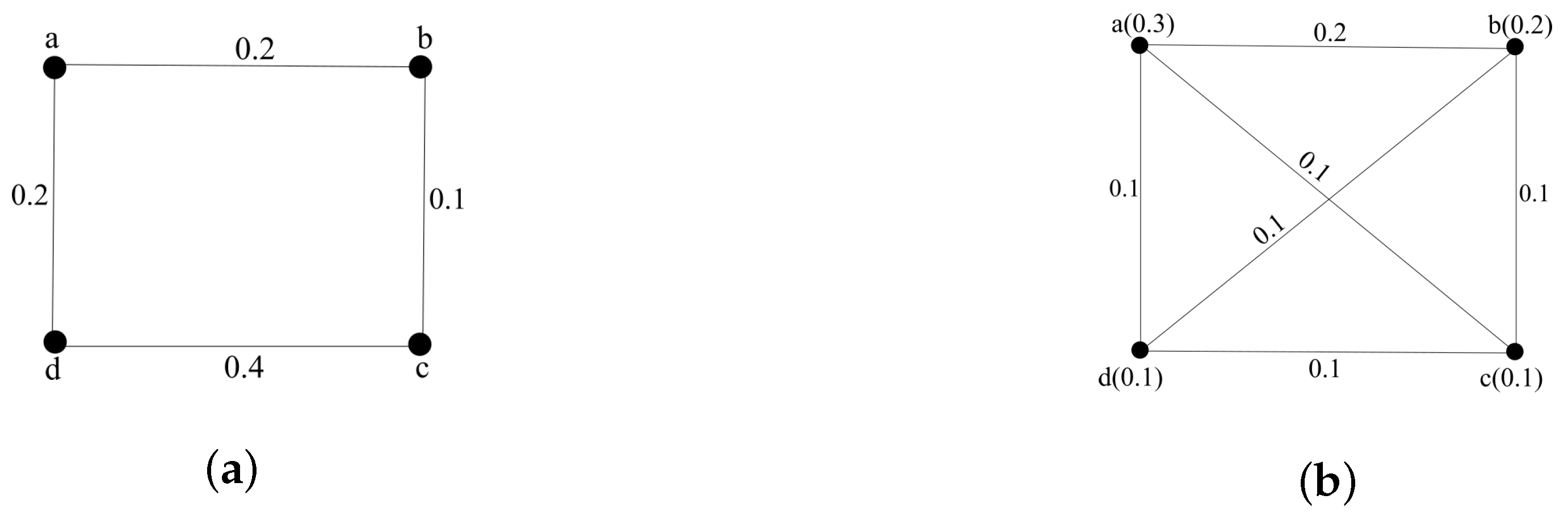
Example 2.

Let $G=(\sigma ,\mu )$ be the fuzzy graph given in Figure 3 with ${\sigma }^{*}=\{a,b,c,d\}.$ Here, ${\mu }^{*}=\{ab,bc,cd,ad,bd\},$ with $\sigma \left(x\right)=1\forall x\in {\sigma }^{*}$ and $\mu \left(ab\right)=0.12,\mu \left(bc\right)=0.13,\mu \left(cd\right)=0.12,$$\mu \left(ad\right)=0.12,$ and $\mu \left(bd\right)=0.05.$ In this fuzzy graph, we can see that $\kappa \left(G\right)=0.24,$${\kappa }_f\left(G\right)=0.1,$${\kappa }^{\prime }\left(G\right)=0.24$ and ${\kappa }_f^{\prime }\left(G\right)=0.13.$

Figure 3. A fuzzy graph with ${\kappa }_f\left(G\right)=0.1$ and ${\kappa }_f^{\prime }\left(G\right)=0.13$.

Theorem 13.

For a connected fuzzy graph $G,$${\kappa }_f\left(G\right)\le \kappa \left(G\right)$ and ${\kappa }_f^{\prime }\left(G\right)\le {\kappa }^{\prime }\left(G\right).$

Proof. 

Let $G=(\sigma ,\mu )$ be a connected fuzzy graph, where ${\sigma }^{*}=\{v_1,v_2,\cdots ,v_n\}.$ Let $X=\{v_1,v_2,\dots ,v_m\}$ be a fuzzy vertex cut with $\kappa \left(G\right)=s\left(X\right).$ So by definition, the removal of X from G reduces the strength of connectedness between some pair of vertices $x,y\in {\sigma }^{*}\setminus X.$ i.e., $CON{N}_{G\setminus X}(x,y)<CON{N}_G(x,y).$ Since we have $w_f\left(X\right)\le s\left(X\right),$ it follows that ${\kappa }_f\left(G\right)=\wedge \{w_f\left(B\right):Bisag-FNCofG\}\le w_f\left(X\right)\le s\left(X\right)=\kappa \left(G\right).$

Let $E=\{e_1,e_2,\dots ,e_n\}$ be a minimum $FEC$ in $G.$ Then, ${\kappa }^{\prime }\left(G\right)=s^{\prime }\left(E\right).$ Also, E satisfies all the conditions for a $g-FEC,$ and hence, ${\kappa }_f^{\prime }\left(G\right)\le {\kappa }^{\prime }\left(G\right).$ □

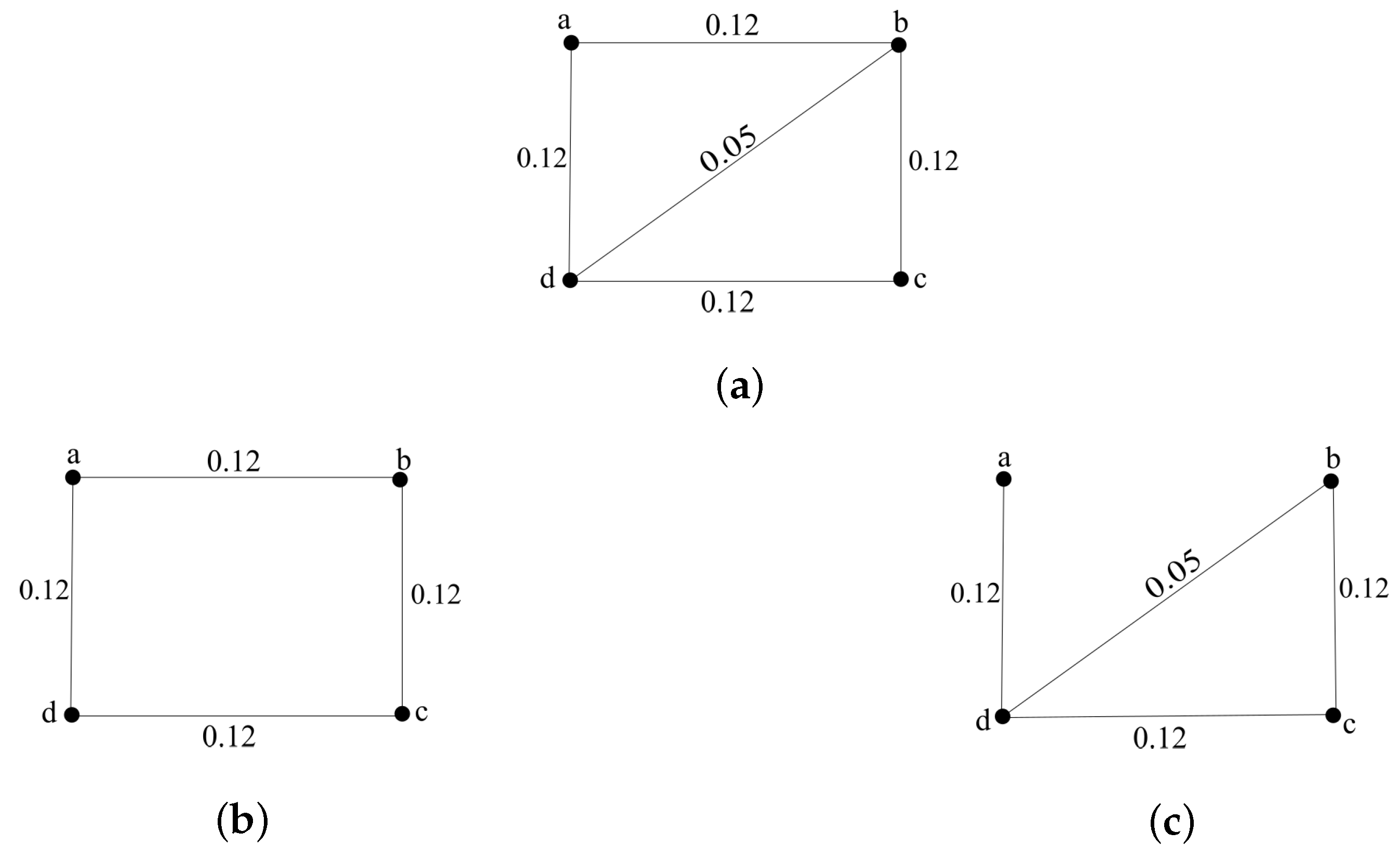
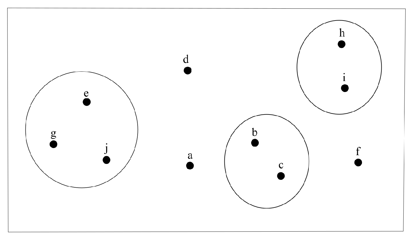
Theorem 1 gives the relationship between vertex connectivity of a fuzzy graph and that of its subgraphs. The below example in Figure 4 shows that this result is not valid in case of a $g-FNC.$

Figure 4. (a) Fuzzy graph with $\kappa \left(G\right)=0.24$ and ${\kappa }_f\left(G\right)=0.1$. (b) $\kappa \left(H\right)=0.24$ and ${\kappa }_f\left(H\right)=0.24$. (c) $\kappa \left(H^{\prime }\right)=0.12$ and ${\kappa }_f\left(H^{\prime }\right)=0.05$.

In this example, ${\kappa }_f\left(H^{\prime }\right)\le {\kappa }_f\left(G\right)\le {\kappa }_f\left(H\right).$ Thus we can see that, for a connected fuzzy graph G with a partial fuzzy subgraph H on the same vertex set, it is not generally true that ${\kappa }_f\left(H\right)\le {\kappa }_f\left(G\right).$ Also it can be seen that ${\kappa }^{\prime }\left(G\right)$ is not always less than or equal to $\lambda \left(G\right)$ in general, but it is always true that ${\kappa }_f^{\prime }\left(G\right)\le \lambda \left(G\right)$ as seen from Theorem 14.

Theorem 14.

For a connected fuzzy graph $G,$${\kappa }_f^{\prime }\left(G\right)\le \lambda \left(G\right).$

Proof. 

Let $G=(\sigma ,\mu )$ be a connected fuzzy graph with edge connectivity $\lambda \left(G\right).$ Let $E=(V_1,V_2)$ be a cut-set in G with weight $\lambda \left(G\right).$ Since E partitions the vertex set into two disjoint sets namely $V_1$ and $V_2,$ the removal of E from G disconnects $G.$ Let $x\in V_1$ and $y\in V_2.$ Then, $CON{N}_{G-E}(x,y)=0<CON{N}_G(x,y).$ Hence, E is a $g-FEC$ in $G.$ Now, ${\kappa }_f^{\prime },$ being the minimum weight of $g-FEC$’s in $G,$ it follows that ${\kappa }_f^{\prime }\left(G\right)\le w_f\left(E\right)=\lambda \left(G\right),$ which completes the proof. □

Combining Theorem 13 and Theorem 14 we have the following result.

Theorem 15.

Let $G=(\sigma ,\mu )$ be a connected fuzzy graph. Then ${\kappa }_f^{\prime }\left(G\right)\le min\{{\kappa }^{\prime }\left(G\right),\lambda \left(G\right)\}$

The existing fuzzy vertex connectivity and fuzzy edge connectivity are related as in the following theorem.

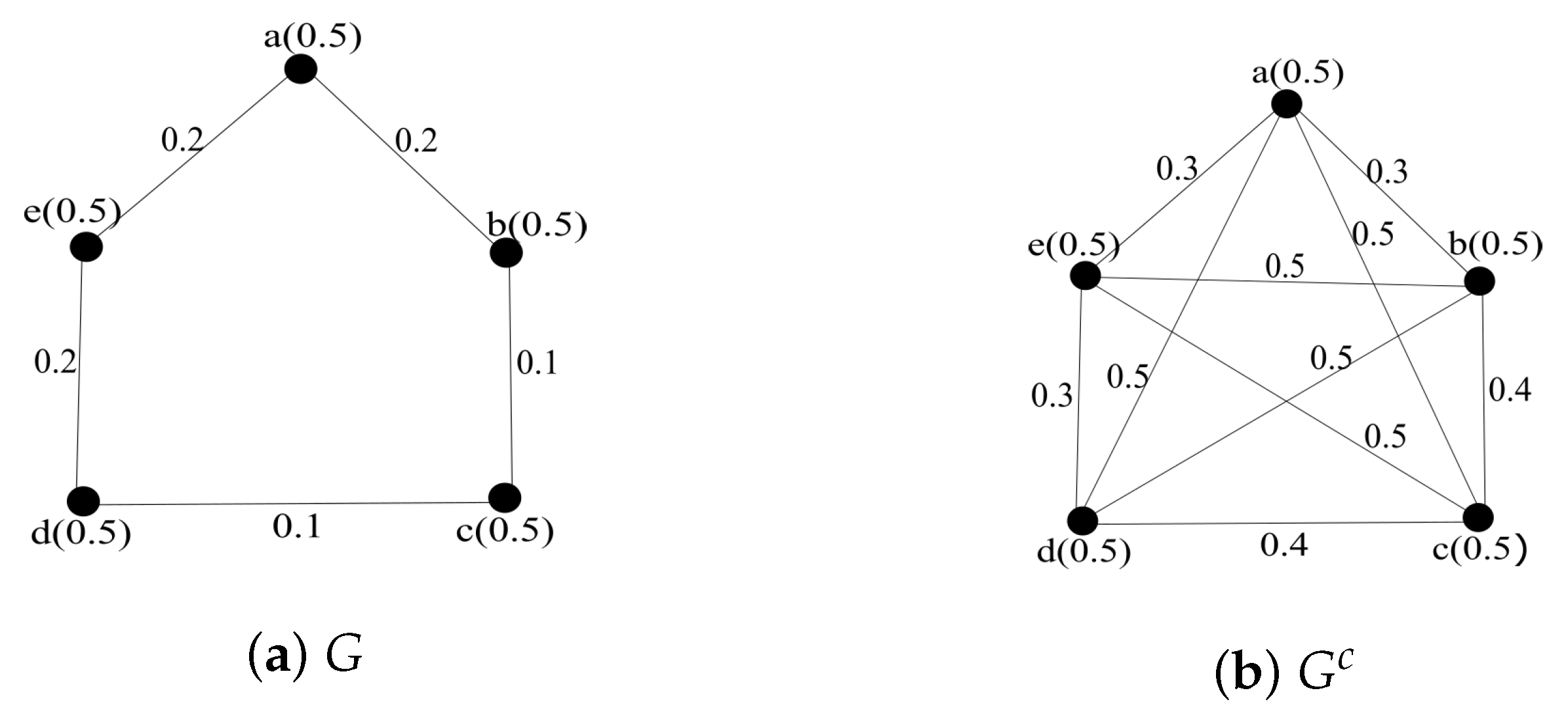
Theorem 16.

[3] In a connected fuzzy graph $G=(\sigma ,\mu ),\kappa \left(G\right)\le {\kappa }^{\prime }\left(G\right).$

As in Theorem 16, we cannot make a general relationship between ${\kappa }_f\left(G\right)$ and ${\kappa }_f^{\prime }\left(G\right).$ This is illustrated in the following example.

Example 3.

Let G=$(\sigma ,\mu )$ be a complete fuzzy graph given in Figure 5 with ${\sigma }^{*}=\{a,b,c,d\}$ and ${\mu }^{*}=\{ab,bc,cd,ad,bd\}.$ Let $\sigma \left(a\right)=0.3,\sigma \left(b\right)=0.2,\sigma \left(c\right)=0.1,\sigma \left(d\right)=0.1$ and $\mu \left(ab\right)=0.2,$$\mu \left(bc\right)=0.1,$$\mu \left(ac\right)=0.1,\mu \left(ad\right)=0.1,\mu \left(bd\right)=0.1$ and $\mu \left(cd\right)=0.1.$ We can see that ${\kappa }_f\left(G\right)=0.3,$ and ${\kappa }_f^{\prime }\left(G\right)=0.2.$

Figure 5. ${\kappa }_f\left(G\right)=0.3,$ and ${\kappa }_f^{\prime }\left(G\right)=0.2$.

Following theorem gives the condition for which ${\kappa }_f\left(G\right)\le {\kappa }_f^{\prime }\left(G\right)$ holds.

Theorem 17.

Let G be a fuzzy graph. If any minimum generalized fuzzy edge cut of G contain more than one element, then ${\kappa }_f\left(G\right)\le {\kappa }_f^{\prime }\left(G\right).$

Proof. 

Let $G=(\sigma ,\mu )$ be a connected fuzzy graph. Let E be a minimum generalized fuzzy edge cut. Then, $w_f^{\prime }\left(E\right)={\kappa }_f^{\prime }.$ Clearly, E does not contain $\alpha$-strong edges, for otherwise, it will contradict the minimality of $E.$ Consider $G-E.$ Then there exist $u,v\in {\sigma }^{*}$ such that $CON{N}_{G-E}(u,v)<CON{N}_G(u,v).$ Let S be the set of end vertices of edges in $E.$ If $u,v\notin S,$ then E is a fuzzy edge cut and hence ${\kappa }^{\prime }\le {\kappa }_f^{\prime }.$ But ${\kappa }_f^{\prime }\le {\kappa }^{\prime }.$ Therefore, ${\kappa }_f^{\prime }={\kappa }^{\prime }.$

Similarly, we can prove that ${\kappa }_f\left(G\right)=\kappa \left(G\right).$ Hence it follows that, ${\kappa }_f\left(G\right)\le {\kappa }_f^{\prime }\left(G\right).$ Either u or v belong to $S.$ Let K be the set of vertices in S which are adjacent either to u or to $v.$ Then $CON{N}_{G-K}(u,v)<CON{N}_G(u,v).$ Therefore, K becomes a $g-FNC$ and hence, ${\kappa }_f^{\prime }={\kappa }^{\prime }.$ Theorem is proved. If G is not connected, then the theorem is trivially true. □

Corollary 1.

If a connected fuzzy graph G contains only $\beta -$strong edges and $\delta -$edges, then ${\kappa }_f\left(G\right)\le {\kappa }_f^{\prime }\left(G\right).$

Proof. 

Let $G=(\sigma ,\mu )$ be a connected fuzzy graph which contain only $\beta -$strong and $\delta -$edges. Then any minimum $g-FEC$ of G contain more than one element, and hence the proof follows by Theorem 17. □

We cannot say anything about the relationship between $g-FNC$ and $g-FEC$ in a connected fuzzy graph $G,$ having a minimum $g-FEC$ containing $\alpha -$strong edges. This is shown in Figure 6.

Figure 6. (a) ${\kappa }_f^{\prime }\left(G\right)=0.2$ and ${\kappa }_f\left(G\right)=0.2$. (b) ${\kappa }_f^{\prime }\left(G\right)=0.2$ and ${\kappa }_f\left(G\right)=0.3$.

Corollary 2.

If a fuzzy graph $G=(\sigma ,\mu )$ satisfies ${\kappa }_f^{\prime }={\kappa }^{\prime },$ then ${\kappa }_f\left(G\right)\le {\kappa }_f^{\prime }\left(G\right).$

Theorem 18.

Let $G=(\sigma ,\mu )$ be a complete fuzzy graph with ${\sigma }^{*}=\{v_1,v_2,\cdots ,v_m\}.$ Let $\sigma \left(v_i\right)=t_i$ for $i=1,2,\cdots ,m$ and $t_1<t_2<\cdots <t_m.$ Then, ${\kappa }_f\left(G\right)=(m-1)t_1$ and ${\kappa }_f^{\prime }\left(G\right)=\wedge \{(m-1)*t_1,$$(m-2)*t_2,$$(m-3)*t_3,\cdots ,2*t_{m-2},t_{m-1}\},$ where * denote the ordinary product.

Proof. 

The first part follows from the fact that any collection of $m-1$ vertices form a minimal $g-FNC$ with weight $(m-1)t_1.$ For the second part, $CON{N}_G(v_i,v_j)=t_i$ as $v_i^{\prime }s$ are arranged in order and G is complete. To reduce $CON{N}_G(v_i,v_j),$ we have to delete a set E of $m-i$ edges incident at $v_i$ with weight $t_i.$ Thus $w_f^{\prime }\left(E\right)=(m-i)*t_i.$ Since $|{\sigma }^{*}|=n,$ there are $\left(\begin{array}{c}n\\ 2\end{array}\right)$$g-$fuzzy edge cuts in $G.$ But they can have weights from the set $\{(m-1)*t_1,(m-2)*t_2,(m-3)*t_3,\cdots ,2*t_{m-2},t_{m-1}\},$ and the proof follows. □

Theorem 19.

For any connected fuzzy graph with generalized fuzzy edge connectivity ${\kappa }_f^{\prime }\left(G\right),$ there exists a connected super fuzzy graph $G^{\prime }$ of G with fuzzy edge connectivity ${\kappa }_f^{\prime }\left(G^{\prime }\right)>{\kappa }_f^{\prime }\left(G\right).$

Proof. Case 1:

For any trivial fuzzy graph with ${\sigma }^{*}=\left\{u\right\},$${\kappa }_f^{\prime }\left(G\right)=0.$ Construct super fuzzy graph as $G^{\prime }=(\rho ,\nu )$ as ${\rho }^{*}={\sigma }^{*}\cup \left\{v\right\}$ and ${\nu }^{*}=\left\{uv\right\}.$ Define,

$$\rho \left(x\right)=\left\{\begin{array}{cc}\sigma \left(x\right)\hfill & ifx=u\hfill \\ 1\hfill & ifx=v\hfill \end{array}\right.$$

and $\nu \left(uv\right)=t,t\in (0,1].$ Clearly ${\kappa }_f^{\prime }\left(G^{\prime }\right)>{\kappa }_f^{\prime }\left(G\right).$

Case 2:

Let G be fuzzy graph with ${\sigma }^{*}=\{u,v\},$ and ${\mu }^{*}=\left\{uv\right\}.$ Thus in this case ${\kappa }_f^{\prime }\left(G\right)=\mu \left(uv\right)=t$(say). Construct a super graph $G^{\prime }=(\rho ,\nu )$ with ${\rho }^{*}={\sigma }^{*}\cup \left\{z\right\}$ and ${\nu }^{*}={\mu }^{*}\cup \{uz,vz\},$ with

$$\rho \left(x\right)=\left\{\begin{array}{cc}\sigma \left(x\right)\hfill & ifx\in {\sigma }^{*}\hfill \\ 1\hfill & ifx=z\hfill \end{array}\right.$$

and

$$\nu \left(xy\right)=\left\{\begin{array}{cc}\mu \left(xy\right)\hfill & ifxy=uv\hfill \\ s\hfill & ifxy=uzxy=vz,s\nleqq t.\hfill \end{array}\right.$$

If $s>t,$ Then, ${\kappa }_f^{\prime }\left(G^{\prime }\right)=s>t={\kappa }_f^{\prime }\left(G\right),$ else then, ${\kappa }_f^{\prime }\left(G^{\prime }\right)=2s>t={\kappa }_f^{\prime }\left(G\right).$

Case 3:

Let G be a fuzzy graph with n vertices say $\{v_1,v_2,\dots ,v_n\},n\ge 3.$ Let $E_1,E_2,\cdots ,E_k$ be minimum generalized fuzzy edge cuts of $G,$ and $X_1,X_2,\cdots ,X_k$ be its end vertices corresponding to each $E_j,j\le k.$ Construct super graphs $G_1,G_2,\cdots ,G_k$ super graphs with $G_k=(\rho ,\nu )$ as ${\rho }^{*}={\sigma }^{*}\cup \left\{z\right\}$ and ${\nu }^{*}={\mu }^{*}\cup \{uz:u\in X_k\}.$

$$\rho \left(x\right)=\left\{\begin{array}{cc}\sigma \left(x\right)\hfill & ifx\in {\sigma }^{*}\hfill \\ \wedge \{\sigma \left(x\right):x\in X_k\}\hfill & ifx=z\hfill \end{array}\right.$$

and

$$\nu \left(xy\right)=\left\{\begin{array}{cc}\mu \left(xy\right)\hfill & ifxy\in {\mu }^{*}\hfill \\ \sigma \left(z\right)\hfill & Otherwise.\hfill \end{array}\right.$$

Thus, every $G_{j}j\ge k,$ we have ${\kappa }_f^{\prime }\left(G_j\right)\ge {\kappa }_f^{\prime }\left(G\right).$ If all ${\kappa }_f^{\prime }\left(G_j\right)={\kappa }_f^{\prime }\left(G\right),$ then $G^{\prime }=\bigcup _{j=1}^k{G}_j$ is super graph with ${\kappa }_f^{\prime }\left(G_j\right)>{\kappa }_f^{\prime }\left(G\right).$

 □

Generalized fuzzy edge connectivity of fuzzy trees coincides with the fuzzy edge connectivity as seen from the following result.

Theorem 20.

For a fuzzy tree $G=(\sigma ,\mu ),{\kappa }_f^{\prime }\left(G\right)=\wedge \{\mu \left(xy\right):xy$ is a strong edge in $G\}.$

Proof. 

Let $G=(\sigma ,\mu )$ be a fuzzy tree. Suppose that G has a cycle, say $C.$ Then there exists a weakest edge $xy$ in $C,$ which is a $\delta -$edge. All other edges in C are strong. Hence the removal of any edge in C other than $xy$ reduces $CON{N}_G(x,y).$ An edge not belonging to a cycle in G is a bridge and hence is a $g-FEC.$

If G has no cycles, then $G^{*}$ is a tree. Every edge of G is bridge and trivially become a $g-FEC.$ Thus it leads to the conclusion that ${\kappa }_f^{\prime }\left(G\right)$ equals to the membership values of strong edges in $G.$ □

As in case of fuzzy node cuts it is not generally true that, for a fuzzy tree ${\kappa }_f\left(G\right)=\wedge \left\{\mathrm{membership}\mathrm{values}\mathrm{of}\mathrm{strong}\mathrm{edges}\mathrm{in}G\right\},$ as seen from the fuzzy graph in Figure 7, whose generalized fuzzy vertex connectivity is $0.1,$ where as the minimum membership value of strong edges in G is $0.2.$ Theorem 21 is trivial.

Figure 7. ${\kappa }_f\left(G\right)=0.1$.

Theorem 21.

For a fuzzy tree $G=(\sigma ,\mu ),$${\kappa }_f^{\prime }(G-uv)\le {\kappa }_f^{\prime }\left(G\right),$ for all $uv\in {\mu }^{*}.$

Theorem 22.

Let $G=(\sigma ,\mu )$ be a fuzzy tree and let $d_s\left(u\right)=d_s\left(v\right)=1,$ for every $\delta -$edge $uv$ in $G.$ Then ${\kappa }_f\left(G\right)=\wedge \{\mu \left(xy\right):xy\mathrm{is}\mathrm{a}\mathrm{strong}\mathrm{edge}\mathrm{in}G\}$.

Proof. 

Consider the fuzzy tree $G=(\sigma ,\mu ).$ Assume the conditions of the theorem. Note that there exist no $g-FNC$ containing the end vertices of $\delta -$edges alone. Consider all strong edges in $G.$ Let $e=xy$ be a strong edge with minimum $\mu -$value. Then either $S_1=\left\{x\right\}$ or $S_2=\left\{y\right\}$ becomes a minimum $g-FNC.$ Precisely, $S_2$ becomes a $g-FNC$ when $d_{\alpha }\left(y\right)=2$ and $S_1$ becomes a $g-FNC$ when $d_{\alpha }\left(x\right)=2.$ Thus ${\kappa }_f\left(G\right)=\wedge \{\mu \left(xy\right):xy\mathrm{is}\mathrm{a}\mathrm{strong}\mathrm{edge}\mathrm{in}G\}$. □

Corollary 3.

Let $G=(\sigma ,\mu )$ be a fuzzy tree such that $G^{*}$ is a cycle, then ${\kappa }_f\left(G\right)=\wedge \{\mu \left(xy\right):xy\mathrm{is}\mathrm{a}\mathrm{strong}\mathrm{edge}\mathrm{in}G\}$

Theorems 23 and 24 show the existance of a generalized $t-$connected and $t-$edge connected complete fuzzy graph for any real $t.$

Theorem 23.

There exists a generalized $t-$connected complete fuzzy graph for any $t\in {\mathrm{I}\mathrm{R}}^{+}.$

Proof. 

Let us first assume that $t\in (0,1].$ A $t-$connected complete fuzzy graph is simply $G=K_2$ with ${\sigma }^{*}=\{u,v\}$ and $\mu \left(uv\right)\ge t.$

Suppose $t\ge 1,$ let $t\in [n,n+1)$ for some $n\in \mathrm{I}\mathrm{N}.$ Model a fuzzy graph G with at least $n+2$ vertices namely $v_1,v_2,\dots ,v_{n+2},\dots ,v_{n+k}.$ Let $\sigma \left(v_i\right)\ge \frac{t}{(n+k)}$ for $i=1,2,\dots ,n+k,$ along with $\mu \left(v_i{v}_j\right)=\sigma \left(v_i\right)\wedge \sigma \left(v_j\right)$ for $i\ne j.$ Then G is a CFG with $n+k$ vertices. Without loss of generality we can assume $v_1$ be the vertex of minimum degree. Thus by Theorem 18, ${\kappa }_f\left(G\right)=(n+k)*\wedge \{\sigma \left(x\right):x\in {\sigma }^{*}\}.$ Thus, ${\kappa }_f\left(G\right)\ge (n+k)*\frac{t}{(n+k)}=t.$ Thus, G is a generalized $t-$connected complete fuzzy graph. □

Theorem 24.

There exists a generalized $t-$edge connected complete fuzzy graph for any $t\in {\mathrm{I}\mathrm{R}}^{+}.$

Proof. 

Let us first assume that $t\in (0,1].$ A generalized $t-$connected complete fuzzy graph is simply $G=K_2$ with ${\sigma }^{*}=\{u,v\}$ and $\mu \left(uv\right)\ge t.$

Suppose $t\ge 1,$ let $t\in [n,n+1)$ for some $n\in \mathrm{I}\mathrm{N}.$ Construct a fuzzy graph G with at least $n+2$ vertices namely $v_1,v_2,\dots ,v_{n+2},\dots ,v_{n+k}.$ Let $\sigma \left(v_i\right)\ge \frac{t}{(n+k)-i}$ for $i=1,2,\dots ,k,k+1$ in a manner that no $v_i$ get he same value. Let $p=\wedge \{\sigma \left(v_i\right):i=1,2,\dots ,k+1\},$$q=\vee \{\sigma \left(v_i\right):i=1,2,\dots ,k+1\}$ and list $\sigma \left(v_i\right)=q\forall v_i$ for $i=k+1,,k+2,\dots ,k+n.$ And now place $\mu \left(v_i{v}_j\right)=\sigma \left(v_i\right)\wedge \sigma \left(v_j\right)$ for $i\ne j.$ By construction G is a complete fuzzy graph. Arrange the vertices in an ascending order of their weights and rename as $u_1,u_2,\dots ,u_{n+k},$$\sigma \left(u_i\right)=t_i$ for $i=1,2,\cdots ,n+k$ and $t_1<t_2<\cdots <t_{k+1}.$ Without loss of generality we can use the Theorem 18 with $n+k$ vertices and ${\kappa }_f^{\prime }\left(G\right)=\wedge \{(n+k-1)*t_1,(n+k-2)*t_2,(n+k-3)*t_3,\cdots ,(n+1)*t_{k-1},\left(n\right)*t_k\}.$ Since $(n+k-j)*t_j=(n+k-j)*\sigma \left(u_j\right)=(n+k-j)*\sigma \left(v_l\right)\ge (n+k-j)*\frac{t}{(n+k)-l}.$ Clearly it can be seen that $(n+k-j)*t_j\ge t$ for any $j,$ as j varies only from $1,2,\dots ,k.$ Thus by definition ${\kappa }_f^{\prime }\left(G\right)\ge t.$ Hence proof follows. □

Theorem 25.

Let $G=(\sigma ,\mu )$ be a fuzzy cycle. Then ${\kappa }_f^{\prime }\left(G\right)=\wedge \{m,2\mu \left(xy\right)\},$ where $xy$ is a weakest edge in $G,$ and m is the minimum membership value of $\alpha -$strong edges in $G.$

Proof. 

Let $G=(\sigma ,\mu )$ be a fuzzy cycle. Then all edges in G are strong. Clearly, any set consisting of a single $\alpha -$ strong edge or two $\beta -$strong edges constitutes $g-FEC$’s in $G.$ Let m be the minimum membership value of $\alpha -$strong edges in G and let $xy$ be an edge of minimum $\mu -$value. Note that any $\beta -$strong edge in G will have membership value $\mu \left(xy\right)$ and any $g-FEC$ containing two $\beta -$ strong edges has strength equal to $2\mu \left(xy\right).$ Then, ${\kappa }_f^{\prime }\left(G\right)=\wedge \{m,2\mu \left(xy\right)\}.$ □

Theorem 26.

Let $G=(\sigma ,\mu )$ be a β-saturated fuzzy cycle. Then ${\kappa }_f^{\prime }(G-v)={\kappa }_f^{\prime }(G-uv)=k$$\forall v\in {\sigma }^{*}$, $uv\in {\mu }^{*}$ where k is the membership value of weakest edge in $G.$

Proof. 

Consider a $\beta$-saturated fuzzy cycle $G,$ then every vertex is adjacent to at least one $\beta$-strong edge. Clearly, the removal of a vertex from G results in a tree. Since G is $\beta -$saturated, $G-u$ has at least one edge say $uv$ such that $\mu \left(uv\right)=k$ where k is the minimum membership value of weakest edge in $G.$ Then by Theorem 14, the result follows. □

Figure 5 shows that the result is true is not true in general. Note that fuzzy graph in Figure 8 is not $\beta -$saturated and Theorem 26 fails.

Figure 8. ${\kappa }_f^{\prime }\left(G\right)=0.4and{\kappa }_f^{\prime }(G-c)=0.4$.

Theorem 27.

Let $G=(\sigma ,\mu )$ be a fuzzy cycle with $|{\sigma }^{*}|=n\ge 5$ and $\sigma \left(u\right)=t,$$t\in (0,1].$ Then for $G^c=(\sigma ,\nu ),$${\kappa }_f\left(G^c\right)\le (n-3)\times \vee \{t-\mu \left(uv\right):\mu \left(uv\right)\ne 0\}.$

Proof. 

Let $G=(\sigma ,\mu )$ be a fuzzy cycle with $|{\sigma }^{*}|=n\ge 5$ and $\sigma \left(u\right)=t,$$t\in (0,1].$ Being a fuzzy cycle G contains only strong edges. Also, $CON{N}_{G^c}(x,y)=t\forall x,y\in {\sigma }^{*}.$ Clearly any $uv\in {\mu }^{*}$ becomes a $\delta -$edge in $G^c,$ and there are exactly $n-3$ strong edges incident at every vertex in $G^c.$ Thus any $g-FNC$X in $G^c$ has cardinality $n-3.$ Also each vertex in X is adjacent with at least one $\delta -$edge whose $\nu -$value is strictly less than $k.$ Let m be the minimum membership value of edges in $G.$ Then, $\nu \left(xy\right)\le t-m\forall xy\in {\mu }^{*}.$ So, ${\kappa }_f\left(G^c\right)\le (n-3)\times \vee \{t-\mu \left(uv\right):\mu \left(uv\right)\ne 0\}.$ □

We can also find a lower bound for the generalized fuzzy vertex connectivity of complements of fuzzy cycles as given in the following theorem. Proof is similar and is omitted.

Theorem 28.

Let $G=(\sigma ,\mu )$ be a fuzzy cycle with $|{\sigma }^{*}|=n\ge 5$ and $\sigma \left(u\right)=t,$$t\in (0,1].$ Then generalized fuzzy vertex connectivity of $G^c=(\sigma ,\nu )$ satisfies ${\kappa }_f\left(G^c\right)\ge (n-3)\times \wedge \{t-\mu \left(uv\right):\mu \left(uv\right)\ne 0\}.$

Definition 3.

Let G be a connected fuzzy graph and $t\in (0,\infty ).$ G is called generalized t-fuzzy connected if ${\kappa }_f\left(G\right)\ge t$ and G is called generalized t-fuzzy edge connected if ${\kappa }_f^{\prime }\left(G\right)\ge t.$

In other words a fuzzy graph G is t-fuzzy connected if there exist no generalized fuzzy vertex cut with weight less than t and is t-fuzzy edge connected if there exist no generalized fuzzy edge cut with weight less than $t.$

Theorem 29.

Every generalized $t-$fuzzy connected graph G is $t-$ connected fuzzy graph.

Proof. 

Let G be a generalized $t-$fuzzy connected graph, so, ${\kappa }_f\left(G\right)\ge t.$ Then by Theorem 13 we have $t\le \kappa \left(G\right).$ Thus G is $t-$connected. □

Below Figure 9 Shows the converse of the above theorem need not true.

Figure 9. $\kappa \left(G\right)=0.24and{\kappa }_f\left(G\right)=0.1$.

In Figure 9, G is $0.23-$connected but it is not generalized $0.23-$fuzzy connected.

5. Algorithm

This section is intended to provide an algorithm for clustering of fuzzy graphs, based on the newly defined connectivity parameters. This algorithm seems to be better than the existing algorithms for fuzzy graph clustering. A comparison is provided. For better understanding we give some of the definitions used in the procedure.

Definition 4.

A generalized $t-$fuzzy edge component of $G=(\sigma ,\mu )$ is a maximal generalized $t-$fuzzy edge connected fuzzy subgraph of $G=(\sigma ,\mu ).$ In other words a maximal generalized $t-$fuzzy edge connected subgraph, is a fuzzy subgraph H of $G,$ induced by a set of vertices in G such that ${\kappa }_f^{\prime }\left(H\right)=t.$

The above concept is illustrated in the following example.

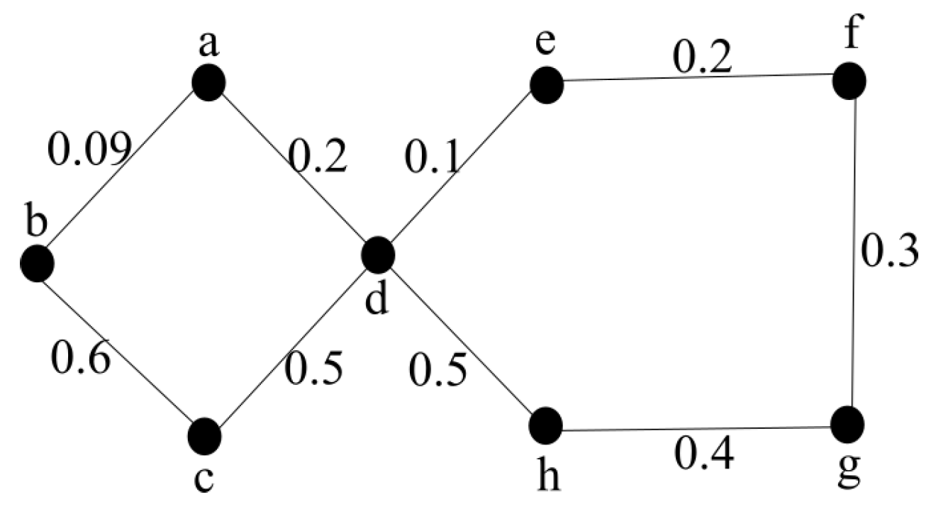
Example 4.

Let G be a fuzzy graph with ${\sigma }^{*}=\{a,b,c,d\}$ and $\sigma \left(x\right)=1\forall x\in {\sigma }^{*},\mu \left(ab\right)=\mu \left(cd\right)=0.2,$$\mu \left(bc\right)=0.5,$ and $\mu \left(ad\right)=0.6.$

Here, ${\kappa }_f^{\prime }\left(G\right)=0.4.$ Hence, G is generalized $t-$fuzzy edge connected for all t such that $t\le 0.4.$ Thus, G itself is a generalized $t-$fuzzy edge component for all t such that $0\le t\le 0.4.$ Now let $t=0.5.$ Then the generalized $0.5-$fuzzy edge components of G are $H_1=\{b,c\},H_2=\left\{a\right\},H_3=\left\{d\right\}$ with ${\kappa }_f^{\prime }\left(H_1\right)=0.5.$ When $t=0.6,$ generalized fuzzy edge components of G are $H_4=\{a,d\},$$H_5=\left\{b\right\}$, $H_6=\left\{c\right\}$ with ${\kappa }_f^{\prime }\left(H_4\right)=0.6.$

Definition 5.

Let $G=(\sigma ,\mu )$ be a fuzzy graph. A collection C of vertices in G is called a generalized fuzzy cluster of level t if the fuzzy subgraph of G induced by C is a generalized $t-$fuzzy edge component of $G.$

We use cohesive matrix M defined by Yeh and Bang [4] to find the maximal $t-$edge connected components of a fuzzy graph $G.$ An element of G is defined to be either a vertex or an edge. The cohesiveness of an element denoted by $h\left(e\right),$ is the maximum value of edge connectivity of the subgraphs of G containing $e.$ And the cohesive matrix M of G is defined as $M=\left(m_{i,j}\right),$ where $m_{i,j}=$ the cohesiveness of the edge $v_i{v}_j$ if $i\ne j$ and the cohesiveness of the vertex $v_i$ if $i=j.$

Now we define generalized cohesive matrix that is used to find maximal generalized $t-$edge connected components of a fuzzy graph $G.$

Definition 6.

Let $G=(\sigma ,\mu )$ be a fuzzy graph. An element of G is defined to be either a vertex or an edge. The generalized cohesiveness of an element denoted by $h\left(e\right),$ is the maximum value of generalized edge connectivity of the subgraphs of G containing $e.$

Definition 7.

Let $G=(\sigma ,\mu )$ be a fuzzy graph. The cohesive matrix M of G is defined as $M=\left(m_{i,j}\right),$ where $m_{i,j}=$ the cohesiveness of the edge $v_i{v}_j$ if $i\ne j$ and the cohesiveness of the vertex $v_i$ if $i=j.$

We use generalized cohesive matrix M to find the maximal generalized $t-$fuzzy edge connected components of a fuzzy graph $G.$

Note that a vertex $v\in {\sigma }^{*}$ is said to be in a cluster of level $t,$ if v belongs to a generalized $t-$fuzzy edge component of $G.$ Thus, finding the generalized $t-$fuzzy edge components of G is equivalent to the extraction of clusters from $G.$ This process of finding generalized $t-$fuzzy edge components and fuzzy clusters using generalized fuzzy edge connectivity is termed $generalizedt-fuzzyedgeconnectivityprocedure.$

Generalized $t-$fuzzy edge connectivity procedure:

Step 1:

Obtain the generalized cohesive matrix M of the fuzzy graph $G.$

Step 2:

Obtain the t-threshold graph $G_t$ of $M.$

Step 3:

The maximal complete subgraphs of $G_t$ are the generalized $t-$fuzzy edge components.

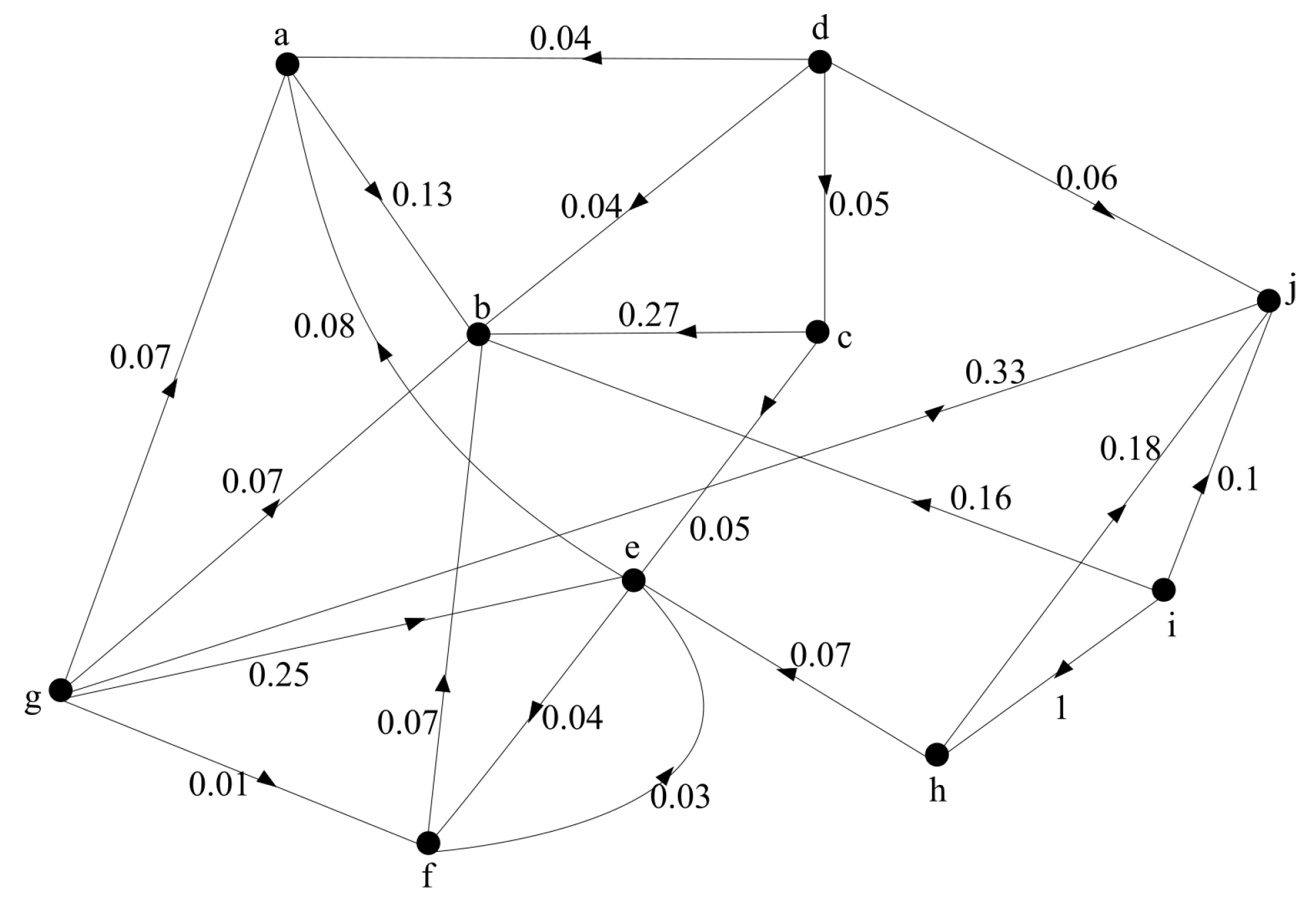
Illustration: Consider the following part of the grid network represented as a fuzzy subgraph given in Figure 10.

Figure 10. A grid network.

The matrix representation of the fuzzy graph in Figure 10 with 10 nodes is,

$$G=\left[\begin{array}{cccccccccc}0& 0.25& 0& 0& 0& 0.45& 0& 0& 0& 0\\ 0.25& 0& 0.3& 0& 0& 0& 0.55& 0& 0& 0\\ 0& 0.3& 0& 0.35& 0& 0& 0& 0.65& 0& 0\\ 0& 0& 0.35& 0& 0.4& 0& 0& 0& 0.75& 0\\ 0& 0& 0& 0.4& 0& 0& 0& 0& 0& 0.8\\ 0.45& 0& 0& 0& 0& 0& 0.25& 0& 0& 0\\ 0& 0.55& 0& 0& 0& 0.25& 0& 0.3& 0& 0\\ 0& 0& 0.65& 0& 0& 0& 0.3& 0& 0.35& 0\\ 0& 0& 0& 0.75& 0& 0& 0& 0.35& 0& 0.4\\ 0& 0& 0& 0& 0.8& 0& 0& 0& 0.4& 0\end{array}\right]$$

The cohesive matrix M of the fuzzy graph in Figure 10 is,

$$M=\left[\begin{array}{cccccccccc}0& 0.5& 0.5& 0.5& 0.5& 0.5& 0.5& 0.5& 0.5& 0.5\\ 0.5& 0& 0.6& 0.6& 0.6& 0.5& 0.6& 0.6& 0.6& 0.6\\ 0.5& 0.6& 0& 0.7& 0.7& 0.5& 0.6& 0.7& 0.7& 0.7\\ 0.5& 0.6& 0.7& 0& 0.8& 0.5& 0.6& 0.7& 0.8& 0.8\\ 0.5& 0.6& 0.7& 0.8& 0& 0.5& 0.6& 0.7& 0.8& 0.8\\ 0.5& 0.5& 0.5& 0.5& 0.5& 0& 0.5& 0.5& 0.5& 0.5\\ 0.5& 0.6& 0.6& 0.6& 0.6& 0.5& 0& 0.6& 0.6& 0.6\\ 0.5& 0.6& 0.7& 0.7& 0.7& 0.5& 0.6& 0& 0.7& 0.7\\ 0.5& 0.6& 0.7& 0.8& 0.8& 0.5& 0.6& 0.7& 0& 0.8\\ 0.5& 0.6& 0.7& 0.8& 0.8& 0.5& 0.6& 0.7& 0.8& 0\end{array}\right]$$

The generalized cohesive matrix M of G is given by,

$$M=\left[\begin{array}{cccccccccc}0& 0.45& 0.45& 0.45& 0.45& 0.45& 0.45& 0.45& 0.45& 0.45\\ 0.45& 0& 0.55& 0.55& 0.55& 0.45& 0.55& 0.55& 0.55& 0.55\\ 0.45& 0.55& 0& 0.65& 0.65& 0.45& 0.55& 0.65& 0.65& 0.65\\ 0.45& 0.55& 0.65& 0& 0.75& 0.45& 0.55& 0.65& 0.75& 0.75\\ 0.45& 0.55& 0.65& 0.75& 0& 0.45& 0.55& 0.65& 0.75& 0.8\\ 0.45& 0.45& 0.45& 0.45& 0.45& 0& 0.45& 0.45& 0.45& 0.45\\ 0.45& 0.55& 0.55& 0.55& 0.55& 0.45& 0& 0.55& 0.55& 0.55\\ 0.45& 0.55& 0.65& 0.65& 0.65& 0.45& 0.55& 0& 0.65& 0.65\\ 0.45& 0.55& 0.65& 0.75& 0.75& 0.45& 0.55& 0.65& 0& 0.75\\ 0.45& 0.55& 0.65& 0.75& 0.8& 0.45& 0.55& 0.65& 0.75& 0\end{array}\right]$$

We consider both clustering procedures given in Reference [3] and the one described above. We can see that the new procedure excels compared to the old.

Generalized $t-$fuzzy connectivity procedure

It is not hard to see that, $K_f^{\prime }\left(G\right)=0.45.$ Using generalized $t-$connectivity procedure we can obtain the generalized fuzzy clusters as follows.

Level	Generalized fuzzy clusters
$(0.8,\infty )$	$\left\{a\right\},\left\{b\right\},\left\{c\right\},\left\{d\right\},\left\{e\right\},\left\{f\right\},\left\{g\right\},\left\{h\right\},\left\{i\right\},\left\{j\right\}$
$(0.75,0.8]$	$\left\{a\right\},\left\{b\right\},\left\{c\right\},\left\{d\right\},\left\{f\right\},\left\{g\right\},\left\{h\right\},\left\{i\right\},\{e,j\}$
$(0.65,0.75]$	$\left\{a\right\},\left\{b\right\},\left\{c\right\},\left\{f\right\},\left\{g\right\},\left\{h\right\},\{d,e,i,j\}$
$(0.55,0.65]$	$\left\{a\right\},\left\{b\right\},\left\{f\right\},\left\{g\right\},\{c,d,e,h,i,j\}$
$(0.45,0.55]$	$\left\{a\right\},\left\{f\right\},\{b,c,d,e,g,h,i,j\}$
$(0,0.45]$	$\{a,b,c,d,e,f,g,h,i,j\}$

Consider the same fuzzy graph used for the above illustration. The clusters obtained while applying $t-$fuzzy edge connectivity procedure in Reference [3] is given below.

$t-$fuzzy edge connectivity procedure

We have $K^{\prime }\left(G\right)=0.5,$ using $t-$fuzzy edge connectivity procedure, we obtain fuzzy clusters as,

Level	Fuzzy clusters
$(0.8,\infty )$	$\left\{a\right\},\left\{b\right\},\left\{c\right\},\left\{d\right\},\left\{e\right\},\left\{f\right\},\left\{g\right\},\left\{h\right\},\left\{i\right\},\left\{j\right\}$
$(0.7,0.8]$	$\left\{a\right\},\left\{b\right\},\left\{c\right\},\left\{f\right\},\left\{g\right\},\left\{h\right\},\{d,e,i,j\}$
$(0.6,0.7]$	$\left\{a\right\},\left\{b\right\},\left\{f\right\},\left\{g\right\},\{c,d,e,h,i,j\}$
$(0.5,0.6]$	$\left\{a\right\},\left\{f\right\},\{b,c,d,e,g,h,i,j\}$
$(0,0.5]$	$\{a,b,c,d,e,f,g,h,i,j\}$

We can observe that the generalized $t-$fuzzy edge connectivity procedure finds more qualitative clusters. For example, the cluster corresponding to the threshold value $t=0.68$ is not present in the second set of clusters. Also note that clusters obtained through the old method appears in the new procedures for lower levels of the thresholds, which is an advantage with regard to the computational complexity involved.

Thus we can see that generalized $t-$fuzzy edge connectivity procedure is more effective than the old $t-$fuzzy edge connectivity procedure in multiple perspectives. In the next section this new clustering technique will be applied in natural human trafficking networks.

6. Application: Human Trafficking

Trafficking of persons is a transnational crime that is often carried out domestically or within a given subregion. Most offenders are convicted in their countries of citizenship. Victims, on the other hand, are often foreigners in the country where their exploitation was detected. Trafficking flows are usually confined to a geographically limited area, either within a country or between neighboring or relatively close countries. In Chapter II of Reference [35], regional overviews are given concerning trafficking situation in four regions, (1) Europe and Central Asia, (2) the Americas, (3) South Asia., East Asia and the Pacific, and (4) Africa and the Middle East. Profiles of offenders, victims, trafficking flows, and regional responses to the trafficking crime are given.

In this section, we proceed with a model given in Reference [36]. In Reference [36], the authors divided the four regions mentioned above further and studied human trafficking between different locations of the globe and represented it as a directed fuzzy graph. Some of the most vulnerable routes are identified and major human trafficking paths are classified. The directed graph $\overrightarrow{G}$ obtained after fuzzyfication is given in Figure 11. In this section, we apply the clustering technique developed in this paper to the said model and draw some conclusions. We use the following subregions: $\left(a\right)$ West-Central Europe, $\left(b\right)$ West-Southern Europe, $\left(c\right)$ Central Europe $\left(d\right)$ Eastern Europe and Central Asia $\left(e\right)$ North and Central America and caribbeans, $\left(f\right)$ South America $\left(g\right)$ East Asia and Pacific $\left(h\right)$ South Asia $\left(i\right)$ Sub Saharan Africa $\left(j\right)$ Middle East.

Figure 11. Directed graph model of human trafficking from Reference [36].

The diagram shows the illegal flow of humans between 10 different subregions of the world. The associated connectivity matrix $A=D_f\left(\overrightarrow{G}\right)$ of the directed fuzzy graph is given below.

$$A=\left[\begin{array}{cccccccccc}0& 0.13& 0& 0& 0& 0& 0& 0& 0& 0\\ 0& 0& 0& 0& 0& 0& 0& 0& 0& 0\\ 0.05& 0.27& 0& 0& 0.05& 0.04& 0& 0& 0& 0\\ 0.05& 0.05& 0.05& 0& 0.05& 0.04& 0& 0& 0& 0.06\\ 0.08& 0.08& 0& 0& 0& 0.04& 0& 0& 0& 0\\ 0.03& 0.07& 0& 0& 0.03& 0& 0& 0& 0& 0\\ 0.08& 0.07& 0& 0& 0.25& 0.04& 0& 0& 0& 0.33\\ 0.07& 0.07& 0& 0& 0.07& 0.04& 0& 0& 0& 0.18\\ 0.07& 0.16& 0& 0& 0.07& 0.04& 0& 1& 0& 0.18\\ 0& 0& 0& 0& 0& 0& 0& 0& 0& 0\end{array}\right]$$

Each entry $a_{ij}$ in A denotes the flow from ith region to jth region. In order to apply the technique developed in this article, the connectivity matrix A of the directed graph is reconstructed by taking $a_{ij}=a_{ji}$ as the connectivity matrix of an un-directed graph as follows. If there is no path from a to $b,$ then the strength from b to a is assigned as $CON{N}_G(a,b).$

$$B=\left[\begin{array}{cccccccccc}0& 0.13& 0.05& 0.05& 0.08& 0.03& 0.08& 0.07& 0.07& 0\\ 0.13& 0& 0.27& 0.05& 0.08& 0.07& 0.07& 0.07& 0.16& 0\\ 0.05& 0.27& 0& 0.05& 0.05& 0.04& 0& 0& 0& 0\\ 0.05& 0.05& 0.05& 0& 0.05& 0.04& 0& 0& 0& 0.06\\ 0.08& 0.08& 0.05& 0.05& 0& 0.04& 0.25& 0.07& 0.07& 0\\ 0.03& 0.07& 0.04& 0.04& 0.04& 0& 0.04& 0.04& 0.04& 0\\ 0.08& 0.07& 0& 0& 0.25& 0.04& 0& 0& 0& 0.33\\ 0.07& 0.07& 0& 0& 0.07& 0.04& 0& 0& 1& 0.18\\ 0.07& 0.16& 0& 0& 0.07& 0.04& 0& 1& 0& 0.18\\ 0& 0& 0& 0.06& 0& 0& 0.33& 0.18& 0.18& 0\end{array}\right]$$

We now apply the new clustering procedure, by finding the cohesiveness matrix. The generalized cohesiveness matrix M for the directed fuzzy graph $\overrightarrow{G}$ is,

$$M=\left[\begin{array}{cccccccccc}0& 0.13& 0.05& 0.05& 0.08& 0.03& 0.08& 0.07& 0.07& 0.08\\ 0.13& 0& 0.27& 0.05& 0.08& 0.07& 0.07& 0.07& 0.16& 0.07\\ 0.05& 0.27& 0& 0.05& 0.05& 0.04& 0.07& 0.07& 0.16& 0.06\\ 0.05& 0.05& 0.05& 0& 0.05& 0.04& 0.06& 0.06& 0.06& 0.06\\ 0.08& 0.08& 0.05& 0.05& 0& 0.04& 0.25& 0.07& 0.07& 0.25\\ 0.03& 0.07& 0.04& 0.04& 0.04& 0& 0.04& 0.04& 0.04& 004\\ 0.08& 0.07& 0.07& 0.06& 0.25& 0.04& 0& 0.07& 0.18& 0.33\\ 0.07& 0.07& 0.07& 0.06& 0.07& 0.04& 0.07& 0& 1& 0.18\\ 0.07& 0.16& 0.16& 0.06& 0.07& 0.04& 0.18& 1& 0& 0.18\\ 0.08& 0.07& 0.05& 0.06& 0.25& 0.04& 0.33& 0.18& 0.18& 0\end{array}\right]$$

Using the algorithm from Reference [6], we have $K_f^{\prime }\left(\overrightarrow{G}\right)=0.03.$ Generalized $t-$connectivity procedure we can produce fuzzy clusters as given bellow.

Level	Fuzzy Clusters
$(1,\infty )$	$\left\{a\right\},\left\{b\right\},\left\{c\right\},\left\{d\right\},\left\{e\right\},\left\{f\right\},\left\{g\right\},\left\{h\right\},\left\{i\right\},\left\{j\right\}$
$(0.33,1]$	$\left\{d\right\},\left\{f\right\},\left\{a\right\},\{b,c\},\left\{e\right\},\left\{g\right\},\left\{j\right\},\{h,i,\}$
$(0.25,0.33]$	$\left\{d\right\},\left\{f\right\},\left\{a\right\},\{b,c\},\left\{e\right\},\{g,j\},\{h,i,\}$
$(0.18,0.25]$	$\left\{d\right\},\left\{f\right\},\left\{a\right\},\{b,c\},\{e,g,j\},\{h,i\}$
$(0.16,0.18]$	$\left\{d\right\},\left\{f\right\},\left\{a\right\},\{b,c\},\{e,g,j\},\{h,i\}$
$(0.13,0.16]$	$\left\{d\right\},\left\{f\right\},\left\{a\right\},\{b,c\},\{e,g,h,i,j\}$
$(0.08,0.13]$	$\left\{d\right\},\left\{f\right\},\{e,g\},\{a,b,c,h,i,j\}$
$(0.07,0.08]$	$\left\{d\right\},\left\{f\right\},\{e,g\},\{a,b,c,h,i,j\}$
$(0.06,0.07]$	$\left\{d\right\},\{a,b,c,e,f,g,h,i,j\}$
$(0.05,0.06]$	$\{a,b,c,d,e,f,g,h,i,j\}$
$(0.04,0.05]$	$\{a,b,c,d,e,f,g,h,i,j\}$
$(0.03,0.04]$	$\{a,b,c,d,e,f,g,h,i,j\}$
$(0,0.03]$	$\{a,b,c,d,e,f,g,h,i,j\}$

Induced subgraph of G with generalized edge connectivity ${\kappa }_f^{\prime }\left(G\right)=0.13$ is given in Figure 12.

Figure 12. Cluster induced subgraph for the level $0.13$.

Cluster of the above subgraph is given in Figure 13.

Figure 13. The Venn Diagram for the graph in Figure 12.

Induced subgraph H of the directed graph G having ${\kappa }_f^{\prime }\left(H\right)=0.18$ is given in Figure 14.

Figure 14. Cluster induced subgraph for the level $0.18$.

Cluster of the above subgraph is given in Figure 15.

Figure 15. The Venn Diagram for the graph in Figure 14.

We can see that there is a moderate flow of humans between most of the locations, except South America, eastern Europe and central Asia. There is a reasonably high flow from the cluster formed by South Asia, Middle East, Sub saharan Africa to North and central America and central Europe to west and Southern Europe. It is possible to assign numerical parameters to the clusters at any level. For example the average cluster density $\rho$ defined by $\frac{n_1*k_1+n_2*k_2+\cdots +n_l*k_l}{n_1+n_2+\cdots +n_l}$ where $n_i$ denote the number of vertices in ith connected component in the cluster induced subgraph and $k_i$ denote the generalized edge connectivity in the ith connected component, gives value $0.16$ for the level $t=0.13$ and $0.47$ for the level $t=0.18.$ More realistic parameters can be defined using cluster size, average distance, and so forth.

7. Conclusions

Graph parameters are extremely important in modeling and controlling dynamic interconnection networks. Widest paths problems and bottleneck problems have been studied widely by computer experts in the past but there were no mathematical theories to substantiate the results until recently. Most of the concepts in the recently introduced fuzzy graph theory can be directly applied to problems which were previously developed algorithmically. This article is an attempt to redefine some of the existing connectivity parameters. The existence of super fuzzy graphs and complete fuzzy graphs with pre-fixed connectivity values are established. Also the existing parametric values are computed for saturated fuzzy cycles and complements of fuzzy graphs. The best possible generalizations for vertex and edge connectivity in graph theory are presented and their values are computed for some of the major sub classes. It is demonstrated with an example that the new values excel the old ones and is helpful in fuzzy graph clustering to find more qualitative clusters. An example, which uses these concepts in the area of human trafficking, is also provided, where the authors are working as a part of a project on sustainable development goals of the United Nations.

References

1. Zadeh, L.A. Fuzzy sets. Inf. Control 1965, 8, 338–353. [Google Scholar] [CrossRef] [Green Version]
2. Rosenfeld, A. Fuzzy graphs. In Fuzzy Sets and Their Applications; Zadeh, L.A., Fu, K.S., Shimura, M., Eds.; Academic Press: New York, NY, USA, 1975; pp. 77–95. [Google Scholar]
3. Mathew, S.; Sunitha, M.S. Node connectivity and arc connectivity in fuzzy graphs. Inf. Sci. 2010, 180, 519–531. [Google Scholar] [CrossRef]
4. Yeh, R.T.; Bang, S.Y. Fuzzy graphs, fuzzy relations, and their applications to cluster analysis. In Fuzzy Sets and Their Applications; Zadeh, L.A., Fu, K.S., Shimura, M., Eds.; Academic Press: New York, NY, USA, 1975; pp. 125–149. [Google Scholar]
5. Bhattacharya, P. Some remarks on fuzzy graphs. Pattern Recognit. Lett. 1987, 6, 297–302. [Google Scholar] [CrossRef]
6. Bhattacharya, P.; Suraweera, F. An algorithm to compute the supremum of max-min powers and a property of fuzzy graphs. Pattern Recognit. Lett. 1991, 12, 413–420. [Google Scholar] [CrossRef]
7. Bhutani, K.R.; Rosenfeld, A. Strong arcs in fuzzy graphs. Inf. Sci. 2003, 152, 319–322. [Google Scholar] [CrossRef]
8. Bhutani, K.R. On automorphisms of fuzzy graphs. Pattern Recognit. Lett. 1989, 9, 159–162. [Google Scholar] [CrossRef]
9. Bhutani, K.R.; Rosenfeld, A. Fuzzy end nodes in fuzzy graphs. Inf. Sci. 2003, 152, 323–326. [Google Scholar] [CrossRef]
10. Bhutani, K.R.; Rosenfeld, A. Geodesics in fuzzy graphs. Electron. Notes Discrete Math. 2003, 15, 51–54. [Google Scholar] [CrossRef]
11. Sunitha, M.S.; Vijayakumar, A. A characterization of fuzzy trees. Inf. Sci. 1999, 113, 293–300. [Google Scholar] [CrossRef] [Green Version]
12. Sunitha, M.S.; Vijayakumar, A. Blocks in fuzzy graphs. J. Fuzzy Math. 2005, 13, 13–23. [Google Scholar]
13. Sunitha, M.S.; Vijayakumar, A. Complement of a fuzzy graph. Indian J. Pure Ap. Mat. 2002, 33, 1451–1464. [Google Scholar]
14. Mathew, S.; Sunitha, M.S. Types of arcs in a fuzzy graph. Inf. Sci. 2009, 179, 1760–1768. [Google Scholar] [CrossRef]
15. Mathew, S.; Sunitha, M.S. Cycle connectivity in fuzzy graphs. J. Intell. Fuzzy Syst. 2013, 24, 549–554. [Google Scholar] [CrossRef]
16. Anjali, N.; Mathew, S. Critical blocks in fuzzy graphs. J. Fuzzy Math. 2015, 23, 907–916. [Google Scholar]
17. Anjali, N.; Mathew, S. On blocks and stars in fuzzy graphs. J. Intell. Fuzzy Syst. 2015, 28, 1659–1665. [Google Scholar] [CrossRef]
18. Mathew, S.; Anjali, N.; Mordeson, J.N. Transitive blocks and their applications in fuzzy interconnection networks. Fuzzy Set. Syst. 2018, in press. [Google Scholar] [CrossRef]
19. Mathew, S.; Sunitha, M.S. A characterization of blocks in fuzzy graphs. J. Fuzzy Math. 2010, 18, 999–1006. [Google Scholar]
20. Mordeson, J.N.; Malik, D.S.; Richards, C.S.; Trebbian, J.A.; Boyce, M.A.; Byrne, M.B.P.; Cousino, B.J. Fuzzy graphs and complentary fuzzy graphs. J. Fuzzy Math. 2016, 24, 271–288. [Google Scholar]
21. Akram, M. Bipolar fuzzy graphs. Inf. Sci. 2011, 181, 5548–5564. [Google Scholar] [CrossRef]
22. Akram, M. Interval-valued fuzzy line graphs. Neural Comput. Appl. 2012, 21, 145–150. [Google Scholar] [CrossRef]
23. Akram, M.; Davvaz, B. Strong intuitionistic fuzzy graphs. Filomat 2012, 26, 177–196. [Google Scholar] [CrossRef] [Green Version]
24. Mathew, S.; Mordeson, J.N.; Malik, D.S. Fuzzy Graph Theory; Springer: Berlin, Germany, 2018. [Google Scholar]
25. Mordeson, J.N.; Nair, P.S. Fuzzy Graphs and Fuzzy Hypergraphs; Physica-Verlag: Heidelberg, Germany, 2000. [Google Scholar]
26. Mordeson, J.N.; Mathew, S.; Malik, D.S. Fuzzy Graph Theory with Applications to Human Trafficking; Springer: Berlin, Germany, 2018. [Google Scholar]
27. Mordeson, J.N. Fuzzy line graphs. Pattern Recognit. Lett. 1993, 14, 381–384. [Google Scholar] [CrossRef]
28. Mordeson, J.N.; Nair, P.S. Cycles and cocycles of fuzzy graphs. Inf. Sci. 1996, 90, 39–49. [Google Scholar] [CrossRef]
29. Binu, M.; Mathew, S.; Mordeson, J.N. Wiener index of a fuzzy graph and application to illegal immigration networks. Fuzzy Set Syst. 2019, 384, 132–147. [Google Scholar]
30. Binu, M.; Mathew, S.; Mordeson, J.N. Connectivity index of a fuzzy graph and its application to human trafficking. Fuzzy Set Syst. 2019, 360, 117–136. [Google Scholar]
31. Binu, M.; Mathew, S.; Mordeson, J.N. Cyclic connectivity index of fuzzy graphs. IEEE T. Fuzzy Syst. 2020. accepted. [Google Scholar] [CrossRef]
32. Mordeson, J.N.; Yao, Y.Y. Fuzzy cycles and fuzzy trees. J. Fuzzy Math. 2002, 10, 189–202. [Google Scholar]
33. Mathew, S.; Mathew, J.K. Saturation in fuzzy graphs. New Math. Nat. Comput. 2018, 1, 113–128. [Google Scholar] [CrossRef]
34. Ali, S.; Mathew, S.; Mordeson, J.N.; Rashmanlou, H. Vertex connectivity of fuzzy graphs with applications to human trafficking. New Math. Nat. Comput. 2018, 14, 457–485. [Google Scholar] [CrossRef]
35. United Nations Office on Drugs and Crime. Global Report on Trafficking in Persons; United Nations Office on Drugs and Crime: Vienna, Austria, 2014. [Google Scholar]
36. Mordeson, J.N.; Mathew, S. Non-deterministic flow in fuzzy networks and its application in identification of human trafficking chains. New Math. Nat. Comput. 2017, 13, 231–243. [Google Scholar] [CrossRef] [Green Version]
Figure 1. A fuzzy graph G having a subgraph H with κ ( H ) > κ ( G ) .
Mathematics 08 00424 g001