Topology in the Alternative Set Theory and Rough Sets via Fuzzy Type Theory

Abstract

In this paper, we will visit Rough Set Theory and the Alternative Set Theory (AST) and elaborate a few selected concepts of them using the means of higher-order fuzzy logic (this is usually called Fuzzy Type Theory). We will show that the basic notions of rough set theory have already been included in AST. Using fuzzy type theory, we generalize basic concepts of rough set theory and the topological concepts of AST to become the concepts of the fuzzy set theory. We will give mostly syntactic proofs of the main properties and relations among all the considered concepts, thus showing that they are universally valid.

1. Introduction

This is a theoretical paper, in which we will visit the well known Rough Set Theory and less known Alternative Set Theory (AST) and show that the basic notions of rough set theory have been included already in AST (though their motivation was different).

Recall that after establishing the rough set theory [1], generalization to its fuzzy version soon appeared (see [2] and the citations therein). This suggests the idea that classical and fuzzy rough set theories can be developed as one formal theory using the formalism of mathematical fuzzy logic. We will do it in this paper using higher-order fuzzy logic (Fuzzy Type Theory; FTT).

AST includes a mathematical model of the vagueness and imprecision phenomena. From this point of view, it has a similar motivation as the fuzzy set theory. Hence, it seems natural to generalize some of the concepts of AST to become the concepts of the fuzzy set theory. We will then formally show the equivalence of them with those of rough set theory.

The goals of this paper are the following:

• Using formalism of FTT, we will unify rough set and fuzzy rough set theories into one formal system. Their concepts can be distinguished only semantically in a model.
• Using formalism of FTT, we will show the equivalence of the concepts of rough set theory with some of the topological concepts introduced earlier in AST. All the considered concepts are then passed into the fuzzy set theory by introducing a proper model.
• We will let the readers know about a very interesting set theory that claims to become an alternative to the classical one, and that has the potential to stand behind foundations of new mathematics.

Our method is simple: the considered concepts of both theories are expressed formally. Therefore, we can directly transform them into the syntax of FTT. Consequently, we obtain fuzzy versions of (the concepts of) both theories. This can be done because the crucial role in both theories is played by the concept of indiscernibility equivalence. As there is the corresponding concept in fuzzy logic, namely fuzzy equality, we use the latter in the mentioned formal definitions. Furthermore, we will mostly prove their properties syntactically and, hence, the results become universally valid in any conceivable model.

For a full understanding of this paper, it is necessary to be acquainted with FTT, which was presented in detail in [3] or [4]. Since the proofs proceed mostly using syntactic means, a detailed presentation of them would be lengthy and tedious. Therefore, in many places, we write “using the properties of FTT” assuming that the reader can finish them him/her-self.

The structure of the paper is the following: In the next two sections, we give a short overview of the rough set theory and AST. We especially present the notions that are elaborated later in Section 5. In Section 4, we provide an overview of the main principles of the fuzzy type theory. As FTT was presented in detail in many papers, our outline is rather brief.

Section 5 is the main contribution of this paper. We transform selected formulas of the rough set theory and AST into the language of FTT. We prove many fundamental properties of the introduced notions (e.g., figure, closure, monad, upper and lower approximation, etc.). Note that these notions and their properties were originally presented and analyzed in the respective theories using only semantic means. Syntactic proofs, together with the completeness theorem, assure us that our results hold in all models. We argue that the use of the language of (mathematical) fuzzy logic suggests more in-depth insight into the character of the discussed concepts and also helps us to better understand why the proved properties hold. At the end of Section 5, we present one (class of a) possible model and demonstrate the studied notions on it.

2. Few Selected Concepts of AST

Though it is not necessary for this paper, we will in this section briefly overview some of the main ideas of AST. Our goal is to let the reader know about this fascinating theory.

The alternative set theory is an attempt to establish a new set theory based on which we could then develop new mathematics. Of course, all of the useful principles of the classical set theory are included, and only some of those leading to counterintuitive results are replaced by more natural ones.

The AST was established by Petr Vopěnka and developed by his school, especially in the 70s and 80s of the previous century. There are many papers published on this theory, and AST is presented in detail in two books [5,6]. Unfortunately, AST was developed in quite difficult times in Czechoslovakia, and so, a few members of the team (including Vopěnka) had limited possibilities to publish and to travel abroad. This is the main reason why the theory did not become popular though being mathematically and philosophically very profound. Still, we believe that in the future it will gain its due attention.

The primary outcome of AST is a new understanding of infinity. In classical set theory, infinity is actual, which means that all elements of a given set, no matter whether it is finite or infinite, are already at one’s disposal. The infinite set is obtained by unlimitedly adding new elements. Of course, such a set can be seen as a whole only by God; we can see its part only. In AST, another concept of infinity called natural infinity is introduced. This kind of infinity can be encountered on large but otherwise classically finite sets.

For example, all atoms forming a visible universe are estimated to be ${10}^{80}$. This number is finite, but it is so large that its end is unreachable for us; any attempt to reach this number by simple counting using even a supercomputer would last longer than the whole universe exists (12.5 $\times {10}^9$ years). Vopěnka also demonstrated that huge sets have virtually the same properties as being classically infinite.

The basic concepts of AST are those of a class and a set. A class X is some actualized grouping of objects that may be delineated unsharply. A set a is a sharp grouping of objects that can be written on a list and for which there is a linear ordering ≤, according to which a has the first as well as last elements. Every set is a class but not vice-versa. A class that is not a set is called proper. A semiset X is a class to which there exists a set a such that $X\subseteq a$. Every set is a semiset, but there also exist proper semisets that are not sets. Semisets are unsharply defined classes.

The fundamental proper semiset is the semiset of finite natural numbers $\mathbb{FN}$. We thus distinguish a proper class (not a semiset) of natural numbers $\mathbb{N}$ and its subclass $\mathbb{FN}\subset \mathbb{N}$. The finite natural numbers $\mathbb{FN}$ form an infinitely countable class, while $\mathbb{N}$ is an uncountable class.

A class X is called set-theoretically definable (we write $\mathrm{sd}\left(X\right)$) if it is defined using a set formula (in a standard way common in the classical set theory). This means that it is sharp. It can be proved that if $\mathrm{sd}\left(X\right)$ and there is a set a such that $X\subseteq a$, then X is a set.

Another essential concept is that of indiscernibility relation (equivalence). It is a class relation

$$\doteq =\bigcap \{R_n\mid n\in \mathbb{FN}\}$$

(1)

where for any $n\in \mathbb{FN}$, $R_n$ is set-theoretically definable, reflexive and symmetric binary relation, $R_{n+1}\subseteq R_n$, and for any elements $x,y,z$, $\langle x,y\rangle \in R_{n+1}$, $\langle y,z\rangle \in R_{n+1}$ implies $\langle x,z\rangle \in R_n$. The informal motivation of this definition is the following: we say that two elements are indiscernible if all sharp criteria that we can distinguish fail. The sharp criteria are modeled by the sharp relations $R_n$.

It can be proved that (1) is an equivalence relation that is a semiset, and it is a mathematical model of the indiscernibility phenomenon. Using it, we can define basic topological concepts. The essential one is the model of a shape that is mathematically grasped by the concept of figure.

Definition 1.

Let ≐ be an indiscernibility equivalence.

(a) 

A figure is a class X fulfilling the following condition:

$$(\forall x)(\forall y)(x\in X\&(x\doteq y)\Rightarrow y\in X).$$

(2)

If X is a class then the figure of X is the class

$$\mathrm{Fig}\left(X\right)=\{x\mid (\exists y\left)\right(y\in X\&(y\doteq x)\left)\right\}.$$

(3)

(b) 

A monad of an element x is a class

$$\mathrm{Mon}\left(x\right)=\{y\mid y\doteq x\}=\mathrm{Fig}\left(\right\{x\left\}\right).$$

(4)

(c) 

Classes$X,Y$are separable,$\mathrm{Sep}(X,Y)$, if there is a set-theoretically definable class Z such that$\mathrm{Fig}\left(X\right)\subseteq Z$and$Z\cap \mathrm{Fig}\left(Y\right)=\varnothing$.

(d) 

Closure of a class X is the class

$$\mathrm{Clo}\left(X\right)=\{x\mid \neg \mathrm{Sep}(\left\{x\right\},X\left)\right\}.$$

Note that the metatheory of AST is classical logic. However, one of the aspects of its motivation is to provide a model of vagueness and imprecision. Therefore, we will transfer these concepts and the basic concepts of rough (fuzzy) set theory into formalism of FTT and show how they are related.

3. Basic Concepts of Rough Set Theory

The rough set theory was introduced by Pavlak in [1]. Its fundamental notion is also indiscernibility equivalence. Let U be a set taken as a universe and let an equivalence relation ≗ be given on U. If $x\in U$, then the equivalence class of x with respect to ≗ is denoted by $\left[x\right]$. Using it, the concepts of upper and lower approximation of a given set are introduced.

Definition 2.

Let $X\subseteq U$ be a set. Then the set

$$\overline{X}=\{u\mid \left[u\right]\cap X\ne \varnothing \}$$

(5)

is called upper approximation, and

$$\underline{X}=\{u\mid \left[u\right]\subseteq X\}$$

(6)

is called lower approximation of X. The boundary region is

$$\mathrm{BN}X:=\mathrm{Up}X\backslash \mathrm{Lo}X.$$

A set is called rough if its boundary region is non-empty, otherwise it is crisp.

Note that

$$\left[u\right]\cap X\ne \varnothing \hspace{1em}\mathrm{iff}\hspace{1em}(\exists v)(v\in [u]\&v\in X)\hspace{1em}\mathrm{iff}\hspace{1em}(\exists v)(v\circeq u\&v\in X).$$

(7)

Similarly

$$\left[u\right]\subseteq X\hspace{1em}\mathrm{iff}\hspace{1em}(\forall v)(v\in [u]\Rightarrow v\in X)\hspace{1em}\mathrm{iff}\hspace{1em}(\forall v)(v\circeq u\Rightarrow v\in X).$$

(8)

The concepts above are, analogously as in AST, defined on the basis of the indiscernibility relation. This is defined on a finite set U of objects using a finite set A of attributes and a set V of values (usually numbers, or some abstract objects). The initial data (they are often called information system) are given by a set of mappings $\{I_a:U\to V\mid a\in A\}$. Then, given a set $P\subseteq A$, an indiscernibility relation ${\circeq }_P$ is

$${\circeq }_P=\{(x,y)\in U^2\mid (\forall a\in P)(I_a\left(x\right)=I_a\left(y\right))\}.$$

(9)

Note that this definition is, in a certain sense, analogous to the definition of indiscernibility relation in AST. While in the latter, we consider a sequence of crisp criteria $R_n$, which by using them we can distinguish the given objects, in rough set theory, we require an equality $I_a\left(x\right)=I_a\left(y\right)$ of values of all attributes $a\in P$. The main difference consists in the finiteness of A. In AST, the sequence $\{R_n\mid n\in \mathbb{FN}\}$ is countably infinite (in the sense of AST), though, of course, restricting this sequence to some finite set is not excluded. Let us emphasize, however, that all the above-considered notions do not depend on the way in which the indiscernibility relation is introduced.

4. Brief Overview of FTT

The first step when defining any (mathematical) fuzzy logic is the definition of an algebra of truth values. Based on it, logical axioms are formulated, and the whole formal system can be developed. In this paper, we need a fuzzy type theory in which the law of double negation holds. This requirement is fulfilled, e.g., by FTT whose truth values form an IMTL-algebra (see [3]). The Łukasiewicz FTT has even more useful properties, and so we will confine to it in this paper. Note that the most general FTT is based on a good EQ_Δ-algebra of truth values (cf. [4]) (Let us remark that we can also introduce a core fuzzy type theory on the basis of which all other kinds of FTT can be obtained—see [7]).

It is important to note that formulas of FTT are interpreted, in general, by functions. Because functions of n variables can be expressed using functions of one variable only (This trick was introduced by M. Schönfinkel, Über die Bausteine der mathematischen Logik. Mathematische Annalen (9)2 (1924), 150–182), we confine in FTT to the latter.

4.1. Truth Degrees

The truth degrees of the Łukasiewicz FTT form a linearly ordered complete MV_Δ-algebra. The latter is the algebra

$${\epsilon }_{\Delta }=\langle E,\vee ,\wedge ,\otimes ,\to ,\mathbf{0},\mathbf{1},\Delta \rangle$$

(10)

fulfilling the following conditions for all $a,b,c\in E$:

(i)

$\langle E,\vee ,\wedge ,\mathbf{0},\mathbf{1}\rangle$ is a bounded lattice (0, 1, are the least and the greatest elements, respectively);

(ii)

$\langle L,\otimes ,\mathbf{1}\rangle$ is a commutative monoid;

(iii)

The operation → is a residuation operation with respect to ⊗, i.e.

$$a\otimes b\le c\hspace{1em}\mathrm{iff}\hspace{1em}a\le b\to c;$$

(iv)

$(a\to b)\vee (b\to a)=\mathbf{1}$;                        (prelinearity)

(v)

$(a\to b)\to b=a\vee b$.

The additional operation $\Delta :E\to E$ is called a (Baaz) delta and for linearly ordered algebras it is defined by

$$\Delta \left(a\right)=\left\{\begin{array}{c}\mathbf{1}\hspace{1em}\mathrm{if}a=\mathbf{1},\hfill \\ \mathbf{0}\hspace{1em}\mathrm{otherwise}.\hfill \end{array}\right.$$

Note that the theory of MV-algebras is well known and described in many papers and books (see, e.g., [8,9] and elsewhere).

A special case is the standard MV_Δ-algebra for which $E=[0,1]$ and the operations are defined as follows:

$$\begin{array}{cccc}\hfill \wedge & =\mathrm{minimum},\hfill & \hfill \vee & =\mathrm{maximum},\hfill \\ \hfill a\otimes b& =0\vee (a+b-1),\hfill & \hfill a\to b& =1\wedge (1-a+b),\hfill \\ \hfill \neg a& =a\to 0=1-a,\hfill & \hfill \Delta \left(a\right)& =\left\{\begin{array}{cc}1\hfill & \mathrm{if}a=1,\hfill \\ 0\hfill & \mathrm{otherwise}.\hfill \end{array}\right.\hfill \end{array}$$

A natural interpretation of logical equivalence in FTT is the operation of biresiduation

$$a\leftrightarrow b=(a\to b)\wedge (b\to a).$$

4.2. Fuzzy Equality

For the semantics of FTT, we also need the concept of a fuzzy equality. It can be defined on an arbitrary set M as a binary fuzzy relation $\doteq :M\times M⟶E$ such that the following holds for all $m,m^{\prime },m^{″}\in M$:

(i)

reflexivity

$$\doteq (m,m)=1;$$

(ii)

symmetry

$$\doteq (m,m^{\prime })=\doteq (m^{\prime },m);$$

(iii)

⊗-transitivity

$$\doteq (m,m^{\prime })\otimes \doteq (m^{\prime },m^{″})\le \doteq (m,m^{″}).$$

We will usually write the truth value of the fuzzy equality between m and $m^{\prime }$ as $[m\doteq m^{\prime }]$, instead of the more precise $\doteq (m,m^{\prime })$. We say that ≐ is separated provided that the equivalence

$$[m\doteq m^{\prime }]=1\hspace{1em}\mathrm{iff}\hspace{1em}m=m^{\prime }$$

holds for all $m,m^{\prime }\in M$.

Let $f,g:M_{\alpha }\to M_{\beta }$ be functions, and let a fuzzy equality ${\doteq }_{\beta }$ on $M_{\beta }$ be given. Then we define the fuzzy equality ${\doteq }_{\beta \alpha }$ between $f,g$ by

$$\left[f{\doteq }_{\beta \alpha }g\right]=\bigwedge \{\left[f\left(x\right){\doteq }_{\beta }g\left(x\right)\right]\mid x\in M_{\alpha }\}.$$

(11)

It can be easily proven that (11) is indeed a fuzzy equality. Moreover, if ${\doteq }_{\beta }$ is separated then (11) is separated, too.

4.3. Syntax

The basic syntactical objects of FTT are those of the classical type theory—see [10], namely the concepts of type and formula. The atomic types are $ϵ$ (elements) and o (truth degrees). Complex types $\left(\beta \alpha \right)$ are formed from the previously formed ones $\beta$ and $\alpha$. The set of all types is denoted by Types.

The language of FTT denoted by J consists of variables $x_{\alpha },\dots$, special constants $c_{\alpha },\dots$ ($\alpha \in$ Types), auxiliary symbol $\lambda$, and brackets. Formulas are formed of variables, constants (each of specific type), and the symbol $\lambda$. Thus, each formula A is assigned a type (we write $A_{\alpha }$). A set of formulas of type $\alpha$ is denoted by Form_α, the set of all formulas by Form. Interpretation of a formula $A_{\beta \alpha }$ is a function from the set of objects of type $\alpha$ into the set of objects of type $\beta$. Thus, if $B\in {Form}_{\beta \alpha }$ and $A\in {Form}_{\alpha }$ then $\left(BA\right)\in {Form}_{\beta }$. Similarly, if $A\in {Form}_{\beta }$ and $x_{\alpha }\in J$, $\alpha \in$Types is a variable and then $\lambda x_{\alpha }{A}_{\beta }\in {Form}_{\beta \alpha }$ is a formula whose interpretation is a function which assigns to each object of type $\alpha$ an object of type $\beta$ represented by the formula $A_{\beta }$.

Remark 1.

Note that each formula is assigned a type. Thus, if $\alpha \in$ Types is a type then $A_{\alpha }$ is a formula of type α. However, to relax the notation from the abundance of subscripts, we will alternatively write $A\in {Form}_{\alpha }$ and understand that A is a formula of type α. If no misunderstanding threatens, in more complex formulas we will often write the type of a subformula at its first occurrence only and omit it in the rest.

It is specific for the type theory that connectives are also formulas. Thus, special formulas (connectives) introduced in FTT are fuzzy equality/equivalence ≡, conjunction ∧, strong conjunction &, disjunction ∨, implication ⇒, and the delta connective Δ, which is interpreted by the delta operation.

Specific constants always present in the language of FTT are the following: ${\mathbf{E}}_{\left(o\alpha \right)\alpha }$, $\alpha \in$ Types (fuzzy equality), ${\mathbf{C}}_{\left(oo\right)o}$ (conjunction), ${\mathbf{S}}_{\left(oo\right)o}$ (strong conjunction), and ${\mathbf{D}}_{oo}$ (delta). The constants ⊤ and $\perp \in {Form}_o$ denote hereditary truth and falsity, respectively.

The fundamental connective in FTT is the fuzzy equality syntactically defined as follows:

(i)

${\equiv }_{\left(oo\right)o}:=\lambda x_o\lambda y_o\left({\mathbf{E}}_{\left(oo\right)o}{y}_o\right)x_o$,

(ii)

${\equiv }_{\left(oϵ\right)ϵ}:=\lambda x_{ϵ}\lambda y_{ϵ}\left({\mathbf{E}}_{\left(oo\right)o}{y}_{ϵ}\right)x_{ϵ}$,

(iii)

${\equiv }_{\left(o\right(\beta \alpha \left)\right)\left(\beta \alpha \right)}:=\lambda f_{\beta \alpha }\lambda g_{\beta \alpha }\left({\mathbf{E}}_{\left(o\right(\beta \alpha \left)\right)\left(\beta \alpha \right)}{g}_{\beta \alpha }\right)f_{\beta \alpha }$.

We will write the fuzzy equality ≡ usually without indicating its type and understand that its type conforms with the type of the connected formulas. We always assume that the interpretation of ≡ is a separated fuzzy equality considered in Section 4.2.

Remark 2.

Note that the fuzzy equality (i) is a logical (fuzzy) equivalence, (ii) fuzzy equality between elements, and (iii) fuzzy equality among functions of type$\beta \alpha$.

Implication is a formula $\Rightarrow \equiv {\lambda x}_o{\lambda y}_o·(x\wedge y)\equiv x$ and negation is $\neg \equiv {\lambda x}_o·x\equiv \perp$. Quantifiers are defined by

$$(\forall x_{\alpha })A_o\equiv (\lambda x_{\alpha }{A}_o\equiv \lambda x_{\alpha }\top ),\hspace{1em}\hspace{1em}\hspace{1em}\hspace{1em}\hspace{1em}\hspace{1em}\hspace{1em}\left(general\right(universal\left)quantifier\right)$$

$$(\exists x_{\alpha })A_o\equiv \neg (\forall x_{\alpha })\neg A_o.\hspace{1em}\hspace{1em}\hspace{1em}\hspace{1em}\hspace{1em}\hspace{1em}\hspace{1em}\hspace{1em}\hspace{1em}\hspace{1em}\hspace{1em}\hspace{1em}\hspace{1em}\left(existentialquantifier\right)$$

Axioms of FTT are presented in detail in [3,4]. They include fundamental axioms characterizing fuzzy equality and functions, axioms of truth values, axioms of delta, quantifiers, and axiom of descriptions.

FTT has two inference rules:

• Rule (R): From $A_{\alpha }\equiv A_{\alpha }^{\prime }$ and $B\in {Form}_o$ infer $B^{\prime }$, where $B^{\prime }$ comes from B by replacing one occurrence of $A_{\alpha }$, which is not preceded by $\lambda$, by $A_{\alpha }^{\prime }$.
• Rule (N): from $A_o$ infer $\Delta A_o$.

A special theory T of FTT (When speaking about a special theory T, we will usually write “a theory T” and omit the adjective “special”.) is a set of formulas of type o (determined by a subset of special axioms, as usual). Provability is defined as usual. If T is a (special) theory and $A_o$ a formula then $T⊢A_o$ means that $A_o$ is provable in T. A theory T is contradictory if $T⊢\perp$. Otherwise it is consistent.

4.4. Semantics

Interpretation of formulas is realized in a general frame which is a tuple

$$\mathcal{M}=\langle {\left(M_{\alpha },{\doteq }_{\alpha }\right)}_{\alpha \in Types},{\epsilon }_{\Delta }\rangle$$

(12)

so that the following holds:

(i)

The ${\epsilon }_{\Delta }$ is a linearly ordered MV_Δ algebra of truth degrees. We put $M_o=E$; $M_{ϵ}$ is a set of arbitrary elements.

(ii)

${\doteq }_{\alpha }:M_{\alpha }\times M_{\alpha }\to E$ is a separated fuzzy equality on $M_{\alpha }$ introduced in Section 4.2.

As a special case, we define: ${\doteq }_o:=\leftrightarrow$ (biresiduation). The fuzzy equality ${\doteq }_{ϵ}$ between elements of type $ϵ$ must be given explicitly. The fuzzy equality between functions $f,f^{\prime }\in M_{\beta \alpha }$ is defined in (11).

(iii)

If $\alpha =\gamma \beta \in Types$ then $M_{\gamma \beta }\subseteq M_{\gamma }^{M_{\beta }}$. As a special case, the set $M_{oo}\cup M_{\left(oo\right)o}$ contains all the operations of the algebra ${\epsilon }_{\Delta }$.

Interpretation of a formula $A_{\alpha }$ in a frame $\mathcal{M}$ is an element from the corresponding set $M_{\alpha }$. It is defined recurrently using an assignment p of elements from $M_{\alpha }$ to variables (of the same type), and we write ${\mathcal{M}}_p\left(A_{\alpha }\right)\in M_{\alpha }$.

More specifically, ${\mathcal{M}}_p\left(A_o\right)\in M_o=E$ and ${\mathcal{M}}_p\left(A_{ϵ}\right)\in M_{ϵ}$. Otherwise, let $\alpha =\gamma \beta$. Then ${\mathcal{M}}_p\left(A_{\gamma \beta }\right)=f\in M_{\gamma \beta }$ where f is a function $f:M_{\beta }\to M_{\gamma }$. If, moreover, $B_{\beta }$ is a formula of type $\beta$ having an interpretation ${\mathcal{M}}_p\left(B_{\beta }\right)=b\in M_{\beta }$, then interpretation ${\mathcal{M}}_p\left(A_{\gamma \beta }{B}_{\beta }\right)$ of the formula $A_{\gamma \beta }{B}_{\beta }$ is a functional value $f\left(b\right)\in M_{\gamma }$ of the function f at point b. Interpretation of the $\lambda$-formula ${\mathcal{M}}_p\left(x_{\alpha }{B}_{\beta }\right)$ is a function $F:M_{\alpha }\to M_{\beta }$ which assigns to each $m_{\alpha }\in M_{\alpha }$ an element $F\left(m_{\alpha }\right)={\mathcal{M}}_{p^{\prime }}\left(B_{\beta }\right)$ determined by an assignment $p^{\prime }$ that is equal to p except for the variable $x_{\alpha }$, for which $p^{\prime }\left(x_{\alpha }\right)=m_{\alpha }$ (For precise definitions see [3].).

A model of a theory T is a general frame $\mathcal{M}$ for which ${\mathcal{M}}_p\left(A_o\right)=$ 1 holds for all axioms $A_o$ of T. A formula $B_o$ is true in the theory T, $T\vDash B_o$, if ${\mathcal{M}}_p\left(B_o\right)=$ 1 in all models $\mathcal{M}$ of T. We will usually consider models in which the algebra ${\epsilon }_{\Delta }$ of truth values is the standard Łukasiewicz one.

The following theorem generalizes the Henkin completeness theorem for classical type theory [11] (cf. also [10]).

Theorem 1.

([3,4])

(a) 

A theory T is consistent iff it has a general model$\mathcal{M}$.

(b) 

For every theory T and a formula$A_o$

$$T⊢A_o\hspace{1em}iff\hspace{1em}T\vDash A_o.$$

We say that a formula $A_o$ is crisp if ${\mathcal{M}}_p\left(A_o\right)\in \{\mathbf{0},\mathbf{1}\}$ in every model $\mathcal{M}$. For example, a formula $\Delta A_o$ is crisp.

Below we will often use the special (derived) formulas ${\mathbf{Y}}_{oo}$ and ${\widehat{\mathbf{Y}}}_{oo}$, by which we can express what the truth value as given in formula $A_o$ has in every model. Their formal definition is ${\mathbf{Y}}_{oo}:=\lambda z_o·\neg \Delta (\neg z_o)$, ${\widehat{\mathbf{Y}}}_{oo}:=\lambda z_o·\neg \Delta (z_o\vee \neg z_o)$. Thus, if $A_o$ is a formula representing a truth value and p is an assignment, then ${\mathcal{M}}_p\left(\widehat{\mathbf{Y}}{A}_o\right)=$ 1 iff ${\mathcal{M}}_p\left(A_o\right)\in (\mathbf{0},\mathbf{1})$ and ${\mathcal{M}}_p\left(\mathbf{Y}{A}_o\right)=$ 1 iff ${\mathcal{M}}_p\left(A_o\right)>0$ holds in any model $\mathcal{M}$. The formulas $\mathbf{Y}{A}_o$ and $\widehat{\mathbf{Y}}{A}_o$ are crisp.

The following lemma will be used below.

Lemma 1.

(a) 

$⊢(\exists z_o)(z_o\equiv y_o)$,

(b) 

$⊢y_o\equiv (\exists z_o)(z_o\&(z_o\equiv y_o))$,

(c) 

$⊢y_o\equiv (\exists z_o)(z_o\&\Delta (z_o\equiv y_o))$,

(d) 

$⊢(\exists z_o)z_o$,

(e) 

If${\mathbf{r}}_o$is a constant then$⊢(\forall x_{\alpha }){\mathbf{r}}_o\equiv {\mathbf{r}}_o$and$⊢(\exists x_{\alpha }){\mathbf{r}}_o\equiv {\mathbf{r}}_o$.

(f) 

$⊢(x_o\equiv y_o)\equiv (\exists z_o)((x_o\equiv z_o)\&(z_o\equiv y_o))$,

(g) 

$⊢x_o\Rightarrow \mathbf{Y}{x}_o$.

Proof. 

(a) follows from the reflexivity of ≡ and ∃-substitution. The proof of (b) is the same as in [12], where the provable property $A_o\Rightarrow (B_o\Rightarrow C_o)⊢A_o\&B_o\Rightarrow C_o)$ must be used. (c) follows from (b). (d) follows from (a) when putting $y_o:=\top$. Similarly for (e) using quantifier axioms and the properties of fuzzy equality. (f) was proved in [12]. (g) follows from the definition $\mathbf{Y}$ using contraposition.  □

5. Rough Sets and AST via Fuzzy Type Theory

5.1. Fuzzy Set Theory in FTT

The fuzzy set theory can be easily formulated using the means of the fuzzy type theory. A fuzzy set in a universe $M_{\alpha }$, $\alpha \in Types$ is obtained by the interpretation of some formula $A_{o\alpha }$. Thus, if a model $\mathcal{M}$ and an assignment p to variables are given, then the interpretation of $A_{o\alpha }$ in $\mathcal{M}$ is the function ${\mathcal{M}}_p\left(A_{o\alpha }\right):M_{\alpha }\to M_o$, which is a fuzzy set in the universe$M_{\alpha }$.

To simplify the explanation, we will not distinguish between a fuzzy set represented by a formula $A_{o\alpha }$ and its interpretation as a fuzzy set. Hence, by abuse of language we will simply say “a fuzzy set $A_{o\alpha }$” and not “a formula $A_{o\alpha }$ whose interpretation is a fuzzy set in the universe $M_{\alpha }$”.

Several basic formal definitions of operations on fuzzy sets are the following:

where $\alpha \in Types$.

Note that the empty and universal fuzzy sets ${\varnothing }_{\alpha }$ and ${\mathbf{V}}_{o\alpha }$ have a type. This means that for each type there are different empty and universal fuzzy sets. This is correct because fuzzy sets are, in fact, functions, which holds also for these special fuzzy sets being identified with constant functions having all values equal to 0 or 1.

The formula $\neg \Delta (z_{o\alpha }\equiv \varnothing )$ expresses that the fuzzy set $z_{o\alpha }$ is nonempty. The complement $\mathbf{V}\backslash A$ of a fuzzy set $A_{o\alpha }$ is represented by a formula

$$\neg A_{o\alpha }:=\lambda u_{\alpha }·\top \&\neg Au.$$

We also need to specify crisp sets: a fuzzy set is crisp if it can be characterized by a formula

$${\mathrm{Crisp}}_{o\left(o\alpha \right)}:=\lambda x_{o\alpha }·(\forall u_{\alpha })(xu\equiv \Delta \left(xu\right)).$$

(13)

The formula $\mathrm{Crisp}$ assigns a truth value to any fuzzy set $x_{o\alpha }$. Hence, saying that $X_{o\alpha }$ is crisp means that $⊢\mathrm{Crisp}{X}_{o\alpha }$, which means that the following is provable:

$$⊢\mathrm{Crisp}{X}_{o\alpha }\equiv (\forall u_{\alpha })\Delta (Xu\equiv \left(Xu\right)).$$

Clearly, ${\mathcal{M}}_p\left(\mathrm{Crisp}{X}_{o\alpha }\right)$ is true in any model $\mathcal{M}$ in which the membership degree ${\mathcal{M}}_p\left(X\right)\left(m\right)\in \{0,1\}$ for all $m\in M_{\alpha }$.

Lemma 2.

For all fuzzy sets$X,Y\in {Form}_{o\alpha }$:

(a) 

$⊢\mathrm{Crisp}{\varnothing }_{o\alpha }$and$⊢\mathrm{Crisp}{\mathbf{V}}_{o\alpha }$.

(b) 

$⊢\mathrm{Crisp}\left(\mathrm{Supp}X\right)$.

(c) 

$⊢X\subseteq \mathrm{Supp}X$.

(d) 

Proof. 

Let $u\in {Form}_{\alpha }$.

(a) This immediately follows from $⊢\perp \equiv \Delta \perp$ and $⊢\top \equiv \Delta \top$.

(b) From the definition, we obtain

$$⊢(\forall u)\left(\right(\mathrm{Supp}X)u\equiv \mathrm{Y}(Xu\left)\right)$$

using the properties of FTT. But since the formula $\left(\mathrm{Y}X\right)u$ is crisp, we have $⊢\mathrm{Y}\left(Xu\right)\equiv \Delta \mathrm{Y}\left(Xu\right)$. From this, using Rule (R) and generalization, we obtain

$$⊢(\forall u)\left(\right(\mathrm{Supp}X)u\equiv \mathrm{Y}(\mathrm{Supp}X\left)u\right)$$

from which $⊢\mathrm{Crisp}\left(\mathrm{Supp}X\right)$ follows.

(c) From Lemma 1g it follows that

$$⊢Xu\Rightarrow \mathrm{Y}\left(Xu\right)$$

from which (b) follows using generalization.

(d) The proof can proceed semantically: let $\mathcal{M}$ be an arbitrary model and p an assignment. Then ${\mathcal{M}}_p\left(\mathrm{Supp}X\right)$ is a crisp set in which the membership degree of any element is either 1 or 0.

Let us denote $⊠\in \{\wedge ,\otimes \}$. Then ${\mathcal{M}}_p\left(\left(\mathrm{Supp}X\right)u\right)⊠{\mathcal{M}}_p\left(Yu\right)=0$ iff, either ${\mathcal{M}}_p\left(Yu\right)=0$ or ${\mathcal{M}}_p\left(\left(\mathrm{Supp}X\right)u\right)=0$, iff ${\mathcal{M}}_p\left(\left(\mathrm{Supp}X\right)u\right)⊠{\mathcal{M}}_p\left(\left(\mathrm{Supp}Y\right)u\right)=0$.  □

A singleton (of type $\alpha$), i.e., a one-element set containing an element of type $\alpha$, is specified in FTT as follows:

$${\mathrm{sg}}_{\left(o\alpha \right)\alpha }{u}_{\alpha }:=\lambda v_{\alpha }·\Delta (u\equiv v).$$

(14)

In words: the interpretation of (14) is a (fuzzy) set of all elements $v\in M_{\alpha }$ equal in the degree 1 to a given element $u\in M_{\alpha }$. By the separation of ${\doteq }_{\alpha }$ (interpretation of ≡), all such elements are classically equal to u, and hence every interpretation of ${\mathrm{sg}}_{\left(o\alpha \right)\alpha }{u}_{\alpha }$ is a one-element set $\left\{u\right\}\subset M_{\alpha }\}$.

Lemma 3.

Let ${\mathrm{sg}}_{\left(o\alpha \right)\alpha }$ be a formula defining a singleton set and $u_{\alpha }$ be a formula of type α.

(a) 

$⊢\mathrm{Crisp}\left(\mathrm{sg}{u}_{\alpha }\right)$.

(b) 

$⊢\mathrm{Supp}\left(\mathrm{sg}u\right)\equiv \mathrm{sg}u$.

Proof. 

(a)

is obvious.

(b)

This follows from the following sequence of provable formulas:

$⊢\mathrm{Supp}\left(\mathrm{sg}u\right)\equiv \lambda v_{\alpha }·\mathrm{Y}\left(\mathrm{sg}u\right)v$, $⊢\mathrm{Supp}\left(\mathrm{sg}u\right)\equiv \lambda v_{\alpha }·\mathrm{Y}(\Delta (u\approx v))$ and

$⊢\mathrm{Supp}\left(\mathrm{sg}u\right)\equiv \mathrm{sg}u$.

 □

5.2. Transfer of Selected Concepts of AST into Fuzzy Set Theory

In this and the following subsections, we will translate several concepts developed in AST and rough set theory into the language of the fuzzy type theory. The outcome is a unified formulation of similar concepts from different theories. Then, when choosing a proper model, we immediately obtain the theory of rough fuzzy sets. Moreover, we will also see that there is a close parallel between topological concepts developed in AST based on the indiscernibility relation and the basic concepts of rough (fuzzy) set theory. This is especially interesting if we realize that AST has been developed earlier than rough set theory and arises from foundations very different from those of the former.

Let us extend the language of FTT by a new fuzzy equality ${\approx }_{\left(o\alpha \right)\alpha }$, $\alpha \in Types$, that fulfills the following axioms for all $t,u,z\in {Form}_{\alpha }$:

(EV1)

$t\approx t$,

(EV2)

$t\approx u\equiv u\approx t$,

(EV3)

$t\approx u\&u\approx z·\Rightarrow t\approx z$,

(EV4)

$\Delta (z\equiv t)\equiv \Delta (z\approx t)$.

Axioms (EV1)–(EV3) are the standard axioms of any fuzzy equality. Axiom (EV4) says that the fuzzy equality ${\approx }_{\left(o\alpha \right)\alpha }$ is separated. In the sequel, we will omit the type $\left(o\alpha \right)\alpha$ at the symbol ≈ and assume that it is always clear from the context.

To simplify the explanation, we will not introduce a special theory but write $⊢A_o$ and understand that $A_o$ is provable in some theory, in which, at least, axioms (EV1)–(EV4) are valid.

Definition 3.

Let$X,Y\in {Form}_{o\alpha }$be fuzzy sets (formulas) and$u\in {Form}_{\alpha }$an element.

(i) 

A figure of a fuzzy set $x_{o\alpha }$ is defined by

$${\mathrm{Fig}}_{\left(o\alpha \right)\left(o\alpha \right)}\equiv \lambda x_{o\alpha }\lambda u_{\alpha }·(\exists v_{\alpha })(xv\&(u\approx v)).$$

(15)

(ii) 

A monad of an element u is defined by

$${\mathrm{Mon}}_{\left(o\alpha \right)\alpha }\equiv \lambda u_{\alpha }\lambda v_{\alpha }·u\approx v.$$

(16)

(iii) 

A property characterizing a fuzzy set to be a figure is represented by the formula

$${\mathbf{FIG}}_{o\left(o\alpha \right)}\equiv {\lambda x}_{o\alpha }·(\forall u_{\alpha })(\forall v_{\alpha })(xu\&(u\approx v)\Rightarrow xv).$$

(17)

By $\lambda$-conversion, a figure of $X\in {Form}_{o\alpha }$ is a fuzzy set

$$⊢\mathrm{Fig}X\equiv \lambda u_{\alpha }·(\exists v_{\alpha })(Xv\&(u\approx v)).$$

At the same time, by $\lambda$-conversion, a monad of $u_{\alpha }$ is a fuzzy set

$$⊢\mathrm{Mon}{u}_{\alpha }\equiv \lambda v_{\alpha }·u\approx v.$$

We say that a fuzzy set $X_{o\alpha }$ is a figure (Note that in the fuzzy set theory, such a fuzzy set is called extensional (w.r.t. ≈).) if

$$⊢\mathbf{FIG}X.$$

Lemma 4.

Let$X,Y\in {Form}_{o\alpha }$and$u,v\in {Form}_{\alpha }$.

(a) 

$⊢\mathbf{FIG}{\varnothing }_{\alpha }$ and $⊢\mathbf{FIG}{\mathbf{V}}_{\alpha }$.

(b) 

$⊢X\subseteq \mathrm{Fig}X$.

(c) 

$⊢\mathbf{FIG}\left(\mathrm{Fig}X\right)$, i.e.,$\mathrm{Fig}X$is a figure.

(d) 

$⊢\mathrm{Fig}\left(\mathrm{sg}u\right)\equiv \mathrm{Mon}u$.

(e) 

If$⊢X\subseteq Y$then$⊢\mathrm{Fig}X\subseteq \mathrm{Fig}Y$.

(f) 

$⊢\mathrm{Fig}(X\cup Y)\equiv (\mathrm{Fig}X\cup \mathrm{Fig}Y)$.

Proof. 

(a) After rewriting, we obtain

$$⊢\mathbf{FIG}{\varnothing }_{\alpha }\equiv (\forall u_{\alpha })(\forall v_{\alpha })({\varnothing }_{\alpha }u\&(u\approx v)\Rightarrow {\varnothing }_{\alpha }v).$$

Due to the definition of ∅, the formula on the right-hand side is equivalent to ⊤, from which (a) follows. For ${\mathbf{V}}_{\alpha }$ the proof is analogous.

(b) This follows from $⊢Xu\&(u\approx u)$

(c) Using $\lambda$-conversion, we obtain from (17) that

$$⊢\mathbf{FIG}\left(\mathrm{Fig}X\right)\equiv (\forall u)(\forall v)\left(\right(\mathrm{Fig}X)u\&u\approx v\Rightarrow (\mathrm{Fig}X\left)v\right)$$

(18)

must be provable. The right-hand side of (18), however, is equivalent to

$$⊢(\exists w)(Xw\&(u\approx v)\&(u\approx w\left)\right)\Rightarrow (\exists w)(Xw\&(v\approx w\left)\right)$$

which is provable using (EV3), the properties of &, and quantifiers.

(d) We start with axiom (EV3):

$$⊢(u\approx w)\&(w\approx v)\Rightarrow u\approx v.$$

Using generalization, the properties of Δ and quantifiers we obtain

$$⊢(\exists w)(\Delta (u\approx w)\&(w\approx v\left)\right)\Rightarrow u\approx v.$$

Conversely, by [12] (Lemma 3(a)), we can prove the opposite implication. Then

$$⊢(\exists w)(\Delta (u\approx w)\&(w\approx v\left)\right)\equiv u\approx v$$

and by generalization and [3] (Theorem 11), we obtain

$$⊢\lambda v·(\exists w)(\Delta (u\approx w)\&(w\approx v\left)\right)\equiv \lambda v·u\approx v.$$

After substitution of the definition of singleton we obtain

$$⊢\lambda v·(\exists w)\left(\right(\mathrm{sg}u)w\&(w\approx v\left)\right)\equiv \lambda v·u\approx v.$$

which is (d) after substituting the definition of a figure.

(e) follows immediately from the definition of $\mathrm{Fig}X$ and the properties of strong conjunction &.

(f) follows from the provable formula

$$⊢(\exists v)\left(\right(Xv\vee Yv)\&(u\approx v\left)\right)\equiv (\exists v)(Xv\&(u\approx v\left)\right)\vee (\exists v)(Yv\&(u\approx v\left)\right)$$

by the properties of FTT ($\lambda$-abstraction).  □

Lemma 5.

Let$X_{o\alpha }$be a fuzzy set. The the following is equivalent.

(a) 

$⊢\mathbf{FIG}X$.

(b) 

$⊢X\equiv \lambda v_{\alpha }·(\exists u)((u\approx v)\&Xu)$.

(c) 

$⊢(\forall u_{\alpha })(Xu\Rightarrow (\mathrm{Mon}u\subseteq X))$.

Proof. 

(a)⇒ (b): Applying (17), we obtain

$$⊢\mathbf{FIG}X\equiv (\forall v)\left(\right(\exists u\left)\right(Xu\&(u\approx v))\Rightarrow Xv).$$

(19)

(b)⇒ (a): Since $⊢(v\approx v)\equiv \top$, using the properties of FTT we can prove that $⊢(\forall v)(Xv\Rightarrow (\exists u\left)\right(Xu\&(v\approx u)\left)\right)$. Joining this and (19), we obtain the first equivalence after application of the properties of FTT.

The equivalence between (b) and (c) follows by the properties of FTT if we realize that $⊢(\mathrm{Mon}u\subseteq X)\equiv (\forall v)\left(\right(u\approx v)\Rightarrow Xv)$.  □

Lemma 6.

Let$X_{o\alpha }$be a fuzzy set.

(a) 

$⊢\mathbf{FIG}\left(X\right)$iff$⊢X\equiv \mathrm{Fig}X$.

(b) 

$⊢\mathrm{Fig}\left(\mathrm{Fig}X\right)\equiv \mathrm{Fig}X$.

Proof. 

(a) Let $⊢\mathbf{FIG}\left(X\right)$. Then

$$⊢(\forall u)(\forall v)(Xu\&u\approx v\Rightarrow Xv)$$

from which

$$⊢(\forall v)\left(\right(\exists u\left)\right(Xu\&u\approx v)\Rightarrow Xv),$$

i.e., $⊢\mathrm{Fig}X\subseteq X$. The converse inclusion follows from Lemma 4(c).

The converse implication follows from Lemma 4(c) and Rule (R).

(b) This follows immediately from Lemma 4(c) and (b).  □

Lemma 7.

$⊢\mathbf{FIG}\left(\mathrm{Mon}{u}_{\alpha }\right)$, i.e., a monad of an element$u_{\alpha }$is a figure.

Proof. 

By Lemma 6(a) we must prove that

$$⊢\mathrm{Mon}{u}_{\alpha }\equiv \mathrm{Fig}\left(\mathrm{Mon}{u}_{\alpha }\right)$$

(20)

After substitution of the definitions of monad and figure, we have

$$⊢\mathrm{Fig}\left(\mathrm{Mon}{u}_{\alpha }\right)\equiv \lambda v_{\alpha }·(\exists z_{\alpha })((u\approx z)\&(z\approx v)),$$

which using [12] (Lemma 3(a)) gives (20).  □

Definition 4.

Let$X,Y\in {Form}_{o\alpha }$be fuzzy sets (formulas) and$u\in {Form}_{\alpha }$an element. Then the following concepts can be introduced:

(i) 

Separability of two fuzzy sets is characterized by the formula

$${\mathrm{Sep}}_{o\left(o\alpha \right)\left(o\alpha \right)}\equiv \lambda x_{o\alpha }\lambda y_{o\alpha }·(\forall v_{\alpha })(\forall v_{\alpha })(\left(\mathrm{Fig}x\right)v\wedge \left(\mathrm{Fig}y\right)w\Rightarrow \neg \mathrm{Y}(v\approx w)).$$

(21)

(ii) 

$X,Y$are separable if$⊢\left(\mathrm{Sep}X\right)Y$.

(iii) 

A special case is separability of an element u from X:

$${\mathrm{Sep}}_{o\alpha \left(o\alpha \right)}\equiv \lambda x_{o\alpha }\lambda u_{\alpha }·(\forall v_{\alpha })(\forall w_{\alpha })(\left(\mathrm{Fig}X\right)v\wedge \left(\mathrm{Mon}u\right)w\Rightarrow \neg \mathrm{Y}(v\approx w)).$$

(22)

(iv) 

Closure of a fuzzy set X is a fuzzy set

$${\mathrm{Clo}}_{(}o\alpha )\left(o\alpha \right)X\equiv \lambda u_{\alpha }·\neg \left(\mathrm{Sep}X\right)u.$$

(23)

Remark 3.

(a) 

Formula (21) means that if fuzzy sets$X_{o\alpha },Y_{o\alpha }$are separated, then if u belongs to$\mathrm{Fig}X$in a non-zero degree and v belongs to$\mathrm{Fig}Y$in a non-zero degree then they cannot be equal in a non-zero degree. Interpretation of this formula, however, can be many-valued, i.e., we can have two fuzzy sets separable only by some degree. Full separability is obtained if provability of$\left(\mathrm{Sep}X\right)Y$is assured—cf. item (ii).

(b) 

Formula (22) is, in fact, different from Formula (21). The special case of the latter is$\left(\mathrm{Sep}X\right)\left(\mathrm{sg}u\right)$. For obvious reasons, however, we will use the same symbol both for separability of two fuzzy sets and separability of an element from a fuzzy set, if no misunderstanding can occur.

If follows from (22) that

$$\neg \left(\mathrm{Sep}X\right)u\equiv (\exists v_{\alpha })(\exists w_{\alpha })((\left(\mathrm{Fig}X\right)v\wedge \left(\mathrm{Mon}u\right)w)\&\mathrm{Y}(v\approx w)).$$

(24)

(c) 

Closure of X is a fuzzy set of elements$u_{\alpha }$, to which there are elements$v_{\alpha }$from the figure$\mathrm{Fig}{X}_{o\alpha }$, and an element$w_{\alpha }$from the monad of$\mathrm{Mon}u$that are fuzzy equal in a non-zero degree.

The following is immediate.

Lemma 8.

$$⊢\left(\mathrm{Clo}X\right)u\equiv (\exists v_{\alpha })(\exists w_{\alpha })((\left(\mathrm{Fig}X\right)v\wedge (u\approx w))\&\mathrm{Y}(v\approx w)).$$

Lemma 9.

Let$X\in {Form}_{o\alpha }$and$u\in {Form}_{\alpha }$.

(a) 

$⊢\mathbf{FIG}\left(\mathrm{Clo}X\right)$, i.e.,$\mathrm{Clo}X$is a figure.

(b) 

$⊢X\subseteq \mathrm{Clo}X$.

(c) 

$⊢\mathrm{Fig}\left(\mathrm{Clo}X\right)\equiv \mathrm{Clo}X$.

(d) 

$⊢\mathrm{Clo}\left(\mathrm{Clo}X\right)\equiv \mathrm{Clo}X$.

(e) 

If X is a figure then$⊢\mathrm{Clo}X\equiv \mathrm{Clo}\left(\mathrm{Fig}X\right)$.

Proof. 

(a) We must prove that

$$⊢(\forall r_{\alpha })(\forall s_{\alpha })(\left(\mathrm{Clo}X\right)r\&(r\approx s)\Rightarrow \left(\mathrm{Clo}X\right)s).$$

(25)

We start with the following provable formula (based on the transitivity of ≈, the properties of FTT and quantifiers):

$$\begin{array}{c}⊢(\exists v_{\alpha })(\exists w_{\alpha })[(\left(\mathrm{Fig}X\right)v\wedge ((r\approx w)\&(r\approx s)))\&\mathrm{Y}(v\approx w)]\Rightarrow \hfill \\ \hfill (\exists v_{\alpha })(\exists w_{\alpha })[(\left(\mathrm{Fig}X\right)v\wedge (w\approx s))\&\mathrm{Y}(v\approx w)]\end{array}$$

(26)

where the right-hand side of the implication is equivalent to $\left(\mathrm{Clo}X\right)s$. The left-hand side is obtained from the provable implication

$$\begin{array}{c}⊢(\exists v_{\alpha })(\exists w_{\alpha })[((\left(\mathrm{Fig}X\right)v\&(r\approx s))\wedge ((r\approx w)\&(r\approx s)))\&\mathrm{Y}(v\approx w)]\Rightarrow \hfill \\ \hfill (\exists v_{\alpha })(\exists w_{\alpha })[(\left(\mathrm{Fig}X\right)v\wedge ((r\approx w)\&(r\approx s)))\&\mathrm{Y}(v\approx w)]\end{array}$$

(27)

in which the provable formula $⊢(A\&C)\wedge (B\&C)\equiv (A\wedge B)\&C$ was used in the left-hand side of (27). Joining the latter with (26) we obtain the implication

$$⊢(\exists v_{\alpha })(\exists w_{\alpha })[(\left(\mathrm{Fig}X\right)v\wedge (r\approx w))\&\mathrm{Y}(v\approx w)\&(r\approx s)]\Rightarrow \left(\mathrm{Clo}X\right)s$$

which, after applying generalization, is equivalent to (25).

(b) Using Lemma 4(b) and the properties of FTT, we obtain the provable formula

$$⊢(Xu\wedge (u\approx u\left)\right)\&\mathrm{Y}(u\approx u)\Rightarrow \left(\right(\mathrm{Fig}X)u\wedge (u\approx u\left)\right)\&\mathrm{Y}(u\approx u).$$

Applying two times substitution to the right-hand side of this implication and using transitivity of ⇒, we obtain the formula

$$⊢Xu\Rightarrow (\exists w)(\exists v)\left[\right(\left(\mathrm{Fig}X\right)v\wedge (u\approx w))\&\mathrm{Y}(v\approx w\left)\right].$$

Finally, using generalization we obtain a formula that is equivalent to (b).

(c) is a consequence of (a) and Lemma 6.

(d) holds if $⊢\left(\mathrm{Clo}\right(\mathrm{Clo}X\left)\right)u\equiv \left(\mathrm{Clo}X\right)u$, where $u\in {Form}_{\alpha }$ is a variable.

The inclusion right to left follows from (b). The opposite inclusion is equivalent to

$$\begin{array}{c}⊢(\exists v)(\exists w)\left(\right(\left(\mathrm{Fig}\right(\mathrm{Clo}X\left)\right)v\wedge (u\approx w))\&\mathrm{Y}(v\approx w\left)\right)\Rightarrow \hfill \\ \hfill (\exists r)(\exists s)\left(\right(\left(\mathrm{Fig}X\right)r\wedge (u\approx s))\&\mathrm{Y}(r\approx s\left)\right).\end{array}$$

(28)

Using (c) and Rule (R), (28) becomes

$$\begin{array}{c}⊢(\exists v)(\exists w)\left[\right[\left[\right(\exists r\left)\right(\exists s\left)\right(\left(\right(\mathrm{Fig}X)r\wedge (v\approx s\left)\right)\&\mathrm{Y}(r\approx s)\left)\right]\wedge (u\approx w)]\&\mathrm{Y}(v\approx w\left)\right]\Rightarrow \hfill \\ \hfill (\exists r)(\exists s)\left(\right(\left(\mathrm{Fig}X\right)r\wedge (u\approx s))\&\mathrm{Y}(r\approx s\left)\right).\end{array}$$

(29)

Using prenex operations, we can rewrite (29) into

$$\begin{array}{c}⊢(\exists v)(\exists w)(\exists r)(\exists s)\left[\right[\left[\right(\left(\mathrm{Fig}X\right)r\wedge (v\approx s))\&\mathrm{Y}(r\approx s\left)\right]\wedge (u\approx w)]\&\mathrm{Y}(v\approx w\left)\right]\Rightarrow \hfill \\ \hfill (\exists r)(\exists s)\left(\right(\left(\mathrm{Fig}X\right)r\wedge (u\approx s))\&\mathrm{Y}(r\approx s\left)\right).\end{array}$$

(30)

Let us denote $D:=(\exists v)(\exists w)(\exists r)(\exists s)\left[\right[\left[\right(\left(\mathrm{Fig}X\right)r\wedge (v\approx s))\&\mathrm{Y}(r\approx s\left)\right]\wedge (u\approx w)]\&\mathrm{Y}(v\approx w\left)\right]$. To prove (30), we start with the provable formula

$$⊢D\Rightarrow (\exists v)(\exists w)(\exists r)(\exists s)\left[\right[\left[\right(\left(\mathrm{Fig}X\right)r\wedge (v\approx s))\&\mathrm{Y}(r\approx s\left)\right]\wedge (u\approx w)]\&\mathrm{Y}(v\approx w\left)\right].$$

(31)

Now, we can consider formulas $\mathrm{Y}(r\approx s),\mathrm{Y}(v\approx w)$ to be equivalent to ⊤ since otherwise they can be equivalent to ⊥ and, consequently, (30) is trivially provable. Using the property $⊢A_o\&\top \equiv A_o$ and the properties of quantifiers, we obtain from (31) the formula

$$⊢D\Rightarrow (\exists v)(\exists w)(\exists r)(\exists s)\left[\right(\mathrm{Fig}X)r\wedge (v\approx s)\wedge (u\approx w\left)\right].$$

After realizing equivalent substitutions, we have

$$⊢D\Rightarrow (\exists w)(\exists r)\left[\right(\mathrm{Fig}X)r\wedge (u\approx w\left)\right]\wedge (\exists v)(\exists s)(v\approx s)$$

(32)

where $⊢(\exists v)(\exists s)(v\approx s)\equiv \top$. We conclude from (32) that

$$⊢D\Rightarrow (\exists w)(\exists r)\left[\right(\mathrm{Fig}X)r\wedge (u\approx w\left)\right].$$

(33)

Renaming bound variables in (33) and adding the formula $\mathrm{Y}(r\approx s),$

$$⊢D\Rightarrow (\exists r)(\exists s)\left[\right(\left(\mathrm{Fig}X\right)r\wedge (u\approx s))\&\mathrm{Y}(r\approx s\left)\right]$$

which proves (d).

(e) follows immediately from Lemma 6 using Rule (R).  □

Definition 5.

Let$X,Y\in {Form}_{o\alpha }$be fuzzy sets (formulas) and$v\in {Form}_{\alpha }$an element.

(i) 

Interior of a fuzzy set:

$${\mathrm{Int}}_{\left(o\alpha \right)\left(o\alpha \right)}:=\lambda x_{o\alpha }\lambda v_{\alpha }·(\exists y_{o\alpha })(\mathbf{FIG}y\wedge (y\subseteq x)\wedge yv).$$

(34)

(ii) 

A fuzzy set Y is dense in X if

$$⊢(Y\subseteq X)\wedge (X\subseteq \mathrm{Clo}Y).$$

(35)

Theorem 2.

Let$X\in {Form}_{o\alpha }$and$u,v\in {Form}_{\alpha }$. Then

(a) 

$⊢{\mathrm{Int}}_{\left(o\alpha \right)\left(o\alpha \right)}{X}_{o\alpha }\equiv \lambda v_{\alpha }·(\exists u_{\alpha })(Xu\wedge (\mathrm{Mon}u\subseteq X)\&\left(\mathrm{Mon}u\right)v).$

(b) 

$⊢{\mathrm{Int}}_{\left(o\alpha \right)\left(o\alpha \right)}{X}_{o\alpha }\equiv \lambda v_{\alpha }·(\exists u_{\alpha })((Xu\wedge (\forall v)(v\approx u\Rightarrow Xv))\&(u\approx v))$.

Proof. 

(a) follows from Definition 5(i) using Lemma 5.

(b) is obtained by rewriting (a).  □

By this theorem, the interior of a fuzzy set X is obtained as a union of all monads contained in it.

Lemma 10.

Let$X\in {Form}_{o\alpha }$and$u,v,w,z\in {Form}_{\alpha }$. A fuzzy set Y is dense in X if$⊢(\forall u)(Yu\Rightarrow Xu)$and

$$⊢(\forall u)[Xu\Rightarrow (\exists z\left)\right(\exists v\left)\right(\exists w\left)\right(\left(\right(Yz\&(v\approx z))\wedge (w\approx u\left)\right)\&(v\approx w)\left)\right].$$

Proof. 

This can be obtained by detailed rewriting of Definition 5(ii).  □

5.3. Rough Fuzzy Sets in FTT

We can define rough fuzzy sets using the formalism of FTT. In the resulting theory we obtain generalization of the original rough set theory.

Definition 6.

The following formulas define special properties of fuzzy sets.

(i) 

Upper approximation of a fuzzy set$x_{o\alpha }$:

$${\mathrm{Up}}_{\left(o\alpha \right)\left(o\alpha \right)}:=\lambda x_{o\alpha }\lambda u_{\alpha }·(\exists v_{\alpha })(xv\&\left(\mathrm{Mon}u\right)v).$$

(36)

(ii) 

Lower approximation of a fuzzy set$x_{o\alpha }$:

$${\mathrm{Lo}}_{\left(o\alpha \right)\left(o\alpha \right)}:=\lambda x_{o\alpha }\lambda u_{\alpha }·(\forall v_{\alpha })(\left(\mathrm{Mon}u\right)v\Rightarrow xv).$$

(37)

When realizing that a monad of $u_{\alpha }$ in (16) is just an equivalence class of $u_{\alpha }$ with regard to ≈, Formulas (36) and (37) are just Formulas (7) and (8) rewritten in the language of FTT. This becomes obvious also from the following lemma.

Lemma 11.

Let$X\in {Form}_{o\alpha }$and$u\in {Form}_{\alpha }$.

(a) 

$\mathrm{Up}X\equiv \lambda u_{\alpha }·(\exists v_{\alpha })(Xv\&(u\approx v))$.

(b) 

$\mathrm{Lo}X\equiv \lambda u_{\alpha }·(\forall v_{\alpha })((u\approx v)\Rightarrow Xv)$.

Proof. 

Obvious.  □

We conclude that Definition 6 indeed defines the concepts of upper and lower approximation of Definition 2 in the formalism of FTT.

Lemma 12.

Let$X\in {Form}_{o\alpha }$.

(a) 

$⊢\mathbf{FIG}\left(\mathrm{Up}X\right)$, i.e.,$\mathrm{Up}X$is a figure.

(b) 

$⊢\mathbf{FIG}\left(\mathrm{Lo}X\right)$, i.e.,$\mathrm{Lo}X$is a figure.

Proof. 

(a) We want to prove that

$$⊢(\forall u)(\forall v)\left(\right(\mathrm{Up}X)u\&(u\approx v\left)\right)\Rightarrow \left(\mathrm{Up}X\right)v.$$

(38)

First note that, after rewriting and by the properties of quantifiers, we obtain

$$⊢(\forall u)(\forall v)\left(\right(\exists z\left)\right(Xz\&(z\approx u))\&(u\approx v\left)\right)\equiv (\forall u)(\forall v)\left(\right(\exists z\left)\right(Xz\&(z\approx u)\&(u\approx v)\left)\right)$$

(39)

Furthermore, using the transitivity of ≈ and the properties of implication, we can prove that

$$⊢Xz\&(z\approx u)\&(u\approx v)\Rightarrow Xz\&(z\approx v).$$

Using generalization and quantifier properties, we obtain

$$⊢(\exists z)(Xz\&(z\approx u)\&(u\approx v\left)\right)\Rightarrow (\exists z)(Xz\&(z\approx v\left)\right).$$

From this, using generalization twice and (39), we obtain (38).

(b) We start with the following provable formula:

$$⊢(v\approx z)\&(u\approx v)\&\left(\right(u\approx z)\Rightarrow Xz)\Rightarrow (u\approx z)\&\left(\right(u\approx z)\Rightarrow Xz).$$

Furthermore, $⊢(u\approx z)\&\left(\right(u\approx z)\Rightarrow Xz)\Rightarrow Xz$. By transitivity of implication and formal adjunction, we obtain from these two formulas that

$$⊢\left(\right(u\approx z)\Rightarrow Xz)\&(u\approx v)\Rightarrow \left(\right(v\approx z)\Rightarrow Xz).$$

Finally, by generalization and properties of quantifiers we obtain

$$(\forall z)\left(\right(u\approx z)\Rightarrow Xz)\&(u\approx v)\Rightarrow (\forall z)\left(\right(v\approx z)\Rightarrow Xz)$$

which is (b).  □

Theorem 3.

Let$X\in {Form}_{o\alpha }$and$u,v\in {Form}_{\alpha }$. Then

$$⊢\mathrm{Up}X\equiv \mathrm{Fig}X.$$

Proof. 

L.1

$⊢\mathrm{Up}X\equiv u·(\exists v)(Xv\&(u\approx v\left)\right)\hspace{1em}\hspace{1em}\hspace{1em}\hspace{1em}\hspace{1em}\hspace{1em}\hspace{1em}\hspace{1em}\hspace{1em}\hspace{1em}\mathrm{Lemma}11\left(\mathrm{a}\right)$

L.2

$⊢\mathrm{Fig}X\equiv \lambda u·(\exists v)(Xv\&(u\approx v\left)\right)\hspace{0.17em}\hspace{0.17em}\hspace{1em}\hspace{1em}\hspace{1em}\hspace{1em}\hspace{1em}\hspace{1em}\hspace{1em}\hspace{1em}\hspace{1em}\mathrm{Lemma}4\left(\mathrm{b}\right)$

L.3

$⊢\mathrm{Up}X\equiv \mathrm{Fig}X\hspace{1em}\hspace{1em}\hspace{1em}\hspace{1em}\hspace{1em}\hspace{1em}\hspace{1em}\hspace{1em}\hspace{1em}\hspace{1em}\hspace{1em}\hspace{1em}\hspace{1em}\mathrm{L}.1,\mathrm{L}.2,\mathrm{Rule}\left(\mathrm{R}\right)$

 □

By this theorem, we see that the concepts of upper approximation from the rough set theory and that of a figure of a (fuzzy) set X from AST are equivalent. It is important to emphasize, however, that the motivation of both concepts is different. While in rough set theory, the goal was to introduce an approximation of a set using an equivalence relation, in AST, the goal was to characterize shapes of objects using the indiscernibility relation. Unlike rough set theory, the latter is an infinitary concept in AST. Namely, it is a mathematical model of the situation in which originally different points begin to merge if any imaginable crisp criteria to discern the objects fail.

The following lemma shows that the basic known properties of rough sets are universally valid.

Lemma 13.

Let$X,Y\in {Form}_{o\alpha }$.

(a) 

$⊢\mathrm{Lo}X\subseteq X$and$⊢X\subseteq \mathrm{Up}X$.

(b) 

$⊢\mathrm{Lo}\varnothing \equiv \varnothing$and$⊢\mathrm{Up}\varnothing \equiv \varnothing$.

(c) 

$⊢\mathrm{Up}(X\cup Y)\equiv (\mathrm{Up}X\cup \mathrm{Up}Y)$.

(d) 

$⊢\mathrm{Lo}(X\cap Y)\equiv (\mathrm{Lo}X\cap \mathrm{Lo}Y)$.

(e) 

$⊢\mathrm{Up}(X\cap Y)\subseteq (\mathrm{Up}X\cap \mathrm{Up}Y)$.

(f) 

$⊢(\mathrm{Lo}X\cup \mathrm{Lo}Y)\subseteq \mathrm{Lo}(X\cup Y)$.

(g) 

$⊢\mathrm{Lo}\left(\mathrm{Lo}X\right)\equiv \mathrm{Lo}X$and$⊢\mathrm{Up}\left(\mathrm{Up}X\right)\equiv \mathrm{Up}X$.

Proof. 

(a) Both inclusions follow from the substitution axioms and the reflexivity of ≈, namely $⊢(u\approx u)\equiv \top$:

$$\begin{array}{cc}\hfill & ⊢(\forall v)\left(\right(u\approx v)\Rightarrow Xu)\Rightarrow \left(\right(u\approx u)\Rightarrow Xu))\hfill \\ \hfill & ⊢Xu\&(u\approx u)\Rightarrow (\exists v)(Xv\&(u\approx v\left)\right)\hfill \end{array}$$

(b) $⊢\mathrm{Lo}\varnothing \equiv \varnothing$ follows from (a). The other equality follows from $⊢(\mathrm{Up}\varnothing )u\equiv (\exists v)(\varnothing u\&$$(u\approx v))$, where the right-hand side is equivalent to ⊥.

(c) follows from Theorem 3 and Lemma 4(f).

(d) will follow if we prove that

$$⊢(\forall v)\left(\right(u\approx v)\Rightarrow (Xv\wedge Yv\left)\right)\equiv (\forall v)\left(\right(u\approx v)\Rightarrow Xv)\wedge (\forall v)\left(\right(u\approx v)\Rightarrow Yv).$$

This formula is implied by the following two provable implications using the quantifier properties:

$$\begin{array}{cc}\hfill \left(\right(u\approx v)\Rightarrow (Xv\wedge Yv\left)\right)\Rightarrow & \left(\right(u\approx v)\Rightarrow Xv)\wedge \left(\right(u\approx v)\Rightarrow Yv),\hfill \\ \hfill \left(\right(u\approx v)\Rightarrow Xv)\wedge \left(\right(u\approx v)\Rightarrow Yv)\Rightarrow & \left(\right(u\approx v)\Rightarrow (Xv\wedge Yv\left)\right).\hfill \end{array}$$

(g) The first formula follows from the provable formula

$$⊢(\forall v_{\alpha })(\forall z_{\alpha })((u\approx v)\&(v\approx z)\Rightarrow Xz)\equiv (\forall z_{\alpha })((u\approx z)\Rightarrow Xz),$$

which is obtained after applying $⊢(u\approx z)\equiv (\exists v)\left(\right(u\approx v)\&(v\approx z\left)\right)$ (cf. [12]).

The second formula is proved analogously.  □

Theorem 4.

Let$X\in {Form}_{o\alpha }$be a fuzzy set and$⊢\mathbf{FIG}X$, i.e., it is a figure..

(a) 

$⊢X\equiv \mathrm{Lo}X$,

(b) 

$⊢\mathrm{Lo}X\equiv \mathrm{Up}X.$

Proof. 

(a) $⊢\mathrm{Lo}X\subseteq X$ by Lemma 13(a).

Let $X\in {Form}_{o\alpha }$ be a figure and $u,v\in {Form}_{\alpha }$. Then

$$⊢(\forall u)(\forall v)(Xu\&(u\approx v)\Rightarrow Xv).$$

From this we obtain

$$⊢Xu\Rightarrow (\forall v)\left(\right(u\approx v)\Rightarrow Xv)$$

using the properties of quantifiers and other properties of FTT. The latter implies the lemma.

(b) by (a), $⊢\mathrm{Lo}X\equiv X$. By Theorem 3, $⊢\mathrm{Up}X\equiv \mathrm{Fig}X$. If X is a figure then $⊢X\equiv \mathrm{Fig}X$ by Lemma 6. Using Rule (R), we have $⊢\mathrm{Lo}X\equiv \mathrm{Fig}X$ and thus $⊢\mathrm{Lo}X\equiv \mathrm{Up}X$.  □

In the same way as in rough set theory we can introduce the fuzzy boundary region and the interior of a fuzzy set.

Definition 7.

Let$X\in {Form}_{o\alpha }$. A boundary regionof X is the fuzzy set

$$\mathrm{BN}X:=\mathrm{Up}X\backslash \mathrm{Lo}X.$$

(40)

It is easy to prove the following.

Lemma 14.

Let$X\in {Form}_{o\alpha }$.

(a) 

If X is a figure, i.e.,$⊢\mathbf{FIG}X$, then$⊢\mathrm{BN}X\equiv \varnothing$.

(b) 

Proof. 

This is obtained by rewriting the corresponding formulas and using the properties of quantifiers. Namely, for all $u,v,w\in {Form}_{\alpha }$, we obtain the following sequence of provable formulas:

The lemma is then obtained by $\lambda$-abstraction.  □

Theorem 5.

Let$X\in {Form}_{o\alpha }$. Then

$$⊢\mathrm{Int}X\equiv \mathrm{Lo}X.$$

Proof. 

By Lemma 13(a), $⊢\mathrm{Lo}X\subseteq X$. Let $u\in {Form}_{\alpha }$. Then $⊢\left(\mathrm{Lo}X\right)u\Rightarrow Xu$, from which $⊢\left(\mathrm{Lo}X\right)v\wedge X_u\equiv Xu$. On the basis of this and using definition of lower approximation, we derive the following sequence of equivalences:

$$\begin{array}{cc}\hfill ⊢\mathrm{Int}X& \equiv \lambda v_{\alpha }·(\exists u_{\alpha })((Xu\wedge (\forall v)(w\approx u\Rightarrow Xv))\&(u\approx v)),\hfill \\ \hfill ⊢\mathrm{Int}X& \equiv \lambda v_{\alpha }·(\exists u_{\alpha })(\left(\mathrm{Lo}X\right)u\&(u\approx v)),\hfill \\ \hfill ⊢\mathrm{Int}X& \equiv \mathrm{Fig}\left(\mathrm{Lo}X\right).\hfill \end{array}$$

The theorem follows from the last equivalence using Lemmas 6 and 12.  □

Thus, by this theorem the concepts of interior and lower approximation are equivalent.

Theorem 6.

Let$X\in {Form}_{o\alpha }$. Then the following is equivalent.

(a) 

$⊢\mathrm{BN}X\equiv \varnothing$.

(b) 

$⊢\mathrm{Lo}X\equiv \mathrm{Up}X$.

(c) 

$⊢\mathbf{FIG}X$.

Proof. 

(a)⇒ (b): Then $⊢(\forall u_{\alpha })(\left(\mathrm{Up}X\right)u\&\left(\mathrm{Lo}X\right)u)\equiv \perp$. By the properties of FTT, this implies that $⊢\mathrm{Up}X\subseteq \mathrm{Lo}X$, which gives (b) by Lemma 13(a).

(b)⇒ (a) follows from the definition difference of fuzzy sets and the fact that $⊢(A_o\&\neg A_o)\equiv \perp$.

(b)⇒ (c): Let $⊢\mathrm{Lo}X\equiv \mathrm{Up}X$. By Lemma 13(a), this implies that $⊢\mathrm{Lo}X\equiv X$. Furthermore, by Theorem 3, $⊢\mathrm{Up}X\equiv \mathrm{Fig}X$ which implies that $⊢\mathrm{Lo}X\equiv \mathrm{Fig}X$ using Rule R and we conclude that $⊢X\equiv \mathrm{Fig}X$ from which $⊢\mathbf{FIG}X$ follows by Lemma 6(a).

(c)⇒ (b) follows from Lemma 14(a).  □

By this theorem, figures have an empty boundary. Following the rough set theory, a fuzzy set is rough if its boundary is non-empty (), i.e., if it is not a figure.

5.4. Model

Let us demonstrate the above notions on a model of FTT. We will construct a model

$${\mathcal{M}}^R=\langle {\left(M_{\alpha },{\doteq }_{\alpha }\right)}_{\alpha \in Types},{\epsilon }_{\Delta }\rangle$$

(cf. (12)) where the algebra of truth values ${\epsilon }_{\Delta }$ is the standard ukasiewicz MV_Δ-algebra and, furthermore,

$$\begin{array}{cccc}\hfill M_o& =[0,1],\hfill & \hfill {\doteq }_o& =\leftrightarrow ,\hfill \\ \hfill M_{ϵ}& =\mathrm{ℝ},\hfill & \hfill {\doteq }_{ϵ}(x,y)& =1-min\{1,|x-y\left|\right\},x,y\in \mathrm{ℝ},\hfill \\ \hfill M_{\beta \alpha }& \subseteq M_{\beta }^{M_{\alpha }},\hfill & \hfill {\doteq }_{\beta \alpha }(f,g)& =\bigwedge \{f\left(x\right){\doteq }_{\beta }g\left(x\right)\mid x\in M_{\alpha }\}\hfill \end{array}$$

where $a\leftrightarrow b=(a\to b)\wedge (b\to a)=1-|a-b|$, $a,b\in [0,1]$, is the operation of biresiduation in ${\epsilon }_{\Delta }$, and ${\doteq }_{\beta \alpha }$ is the fuzzy equality (11). The sets $M_{\beta \alpha }$ are supposed to contain all functions $f:M_{\alpha }\to M_{\beta }$ so that all formulas $B_{\beta \alpha }$ are assured to have a value in $M_{\beta \alpha }$ (Note that such a definition of a model of FTT generalizes the concept of a safe model of fuzzy predicate logic introduced by Hájek in [9].).

For simplicity, we will put ${\mathcal{M}}_p^R(\approx )={\mathcal{M}}_p^R(\equiv )$ where p is an assignment of values from ${\mathcal{M}}^R$ to variables. Hence, axioms (EV1)–(EV4) are trivially true in ${\mathcal{M}}^R$ and, therefore, it is a model of our theory. Fuzzy sets on arbitrary universe $M_{\alpha }$ are functions from the set $M_{o\alpha }$ that are obtained as interpretation ${\mathcal{M}}_p^R\left(A_{o\alpha }\right)$ of certain formulas $A_{o\alpha }$.

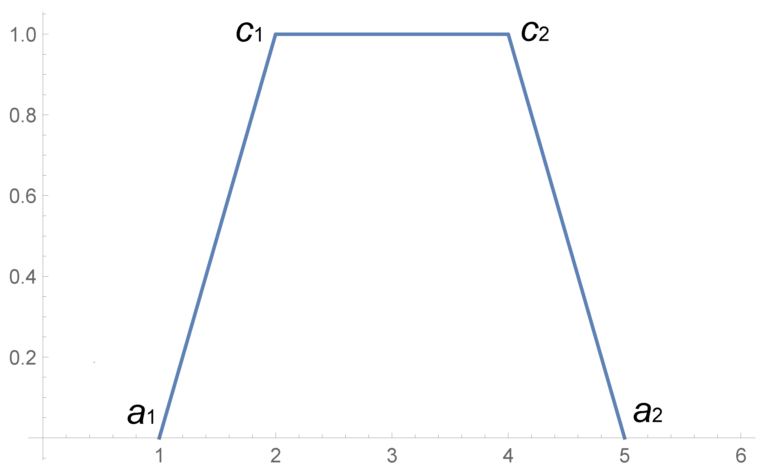
Let us define the function ${\mathsf{\Pi }}_{a_1,c_1,c_2,a_2}:\mathrm{ℝ}\to [0,1]$ by

$${\mathsf{\Pi }}_{a_1,c_1,c_2,a_2}\left(z\right)=\left\{\begin{array}{cc}0\hfill & z<a_1\mathrm{or}{a}_2<z,\hfill \\ 1\hfill & z\in [c_1,c_2],\hfill \\ \frac{z-a_1}{c_1-a_1}\hfill & z\in [a_1,c_1],\hfill \\ \frac{a_2-z}{a_2-c_2}\hfill & z\in [c_2,a_2]\hfill \end{array}\right.$$

where $a_1\le c_1\le c_2\le a_2$ are parameters. The function is a simple trapezoidal function depicted in Figure 1.

Proposition 1.

Let$A\in {Form}_{oϵ}$be a formula whose interpretation in the model${\mathcal{M}}^R$is a fuzzy set with the membership function${\mathcal{M}}^R\left(A\right)={\mathsf{\Pi }}_{a_1,c_1,c_2,a_2}$, provided that$c_1-a_1\ge 1$as well as$a_2-c_2\ge 1$. Then${\mathcal{M}}^R\left(A\right)$is a figure in the model${\mathcal{M}}^R$, i.e.,${\mathcal{M}}_p^R\left(\mathbf{FIG}A\right)=1$.

Proof. 

We must check that for all $x,y\in \mathrm{ℝ}$,

$${\mathcal{M}}_p^R\left(A\right)\left(x\right)\otimes (1-min\{1,|x-y|\left\}\right)\le {\mathcal{M}}_p^R\left(A\right)\left(y\right).$$

To prove this inequality is a tedious but straightforward task.  □

Let us consider a fuzzy set $X\in {Form}_{oϵ}$.

(i)

Let the interpretation ${\mathcal{M}}_p^R\left(X\right)=[c1,c2]$ (a set). Then interpretation ${\mathcal{M}}_p^R\left(\mathrm{Fig}X\right)$ of a figure of X is a fuzzy set depicted in Figure 2.

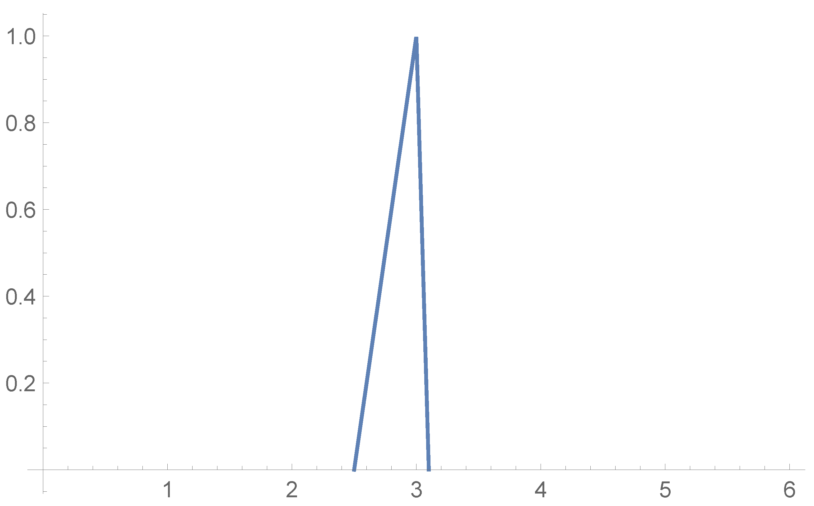
(ii)

Let the interpretation ${\mathcal{M}}_p^R\left(X\right)$ be

$${\mathcal{M}}_p^R\left(X\right)\left(z\right)=\left\{\begin{array}{cc}1-\frac{x_0-z}{0.5}\hfill & z\in [x_0-0.5,x_0],\hfill \\ 1-\frac{z-x_0}{0.1}\hfill & z\in [x_0,x_0+0.1],\hfill \\ 0\hfill & \mathrm{otherwise}\hfill \end{array}\right.$$

(41)

where $x_0\in \mathrm{ℝ}$. This fuzzy set is depicted in Figure 3. Then interpretation ${\mathcal{M}}_p^R\left(\mathrm{Fig}X\right)$ of a figure of X is a fuzzy set depicted in Figure 4.

6. Conclusions

This paper focuses on a few concepts of two, originally unrelated theories: the Rough Set Theory and the Alternative Set Theory. It turns out that the topology in AST has been developed using the notion of indiscernibility relation (equivalence), which is also the leading notion in rough set theory.

Our core idea is a translation of some concepts developed in AST and rough sets, which are formulated using logical formulas, into the language of fuzzy type theory. We thus obtain a unified formulation of similar concepts from different theories and, after choosing a proper model, we get either classical or rough fuzzy set theories enriched by the concepts of AST. Moreover, we learned that the concepts of upper approximation and figure coincide and that many properties of all the concepts have a general validity because they are proved syntactically.

We can continue the development of our theory by introducing further (fuzzy) topological concepts, e.g., closed and open fuzzy sets (a fuzzy set $X_{o\alpha }$ is closed if $⊢X\equiv \mathrm{Clo}X$ and open if $\mathbf{V}\backslash X$ is closed), or connected fuzzy sets, etc. This may be the topic of some of the future papers.

One of the author’s old ideas is finding a bridge between the concepts of a semiset (the crucial concept of AST) and a fuzzy set. This problem has been partially solved in [13,14] (Chapter 4). Fuzzy sets are constructed there as approximations of semisets within AST. The present paper also suggests another principle, namely, to interpret axioms of AST in a special model of FTT and, hence, to obtain fuzzy sets as the natural pendant of semisets. This topic will be the focus of some of the future papers.