Article

Global Mittag–Leffler Stability and Stabilization Analysis of Fractional-Order Quaternion-Valued Memristive Neural Networks

by
Grienggrai Rajchakit
1,*,
Pharunyou Chanthorn
2,
Pramet Kaewmesri
3,
Ramalingam Sriraman
4 and
Chee Peng Lim
5
1
Department of Mathematics, Faculty of Science, Maejo University, Chiang Mai 50290, Thailand
2
Research Center in Mathematics and Applied Mathematics, Department of Mathematics, Faculty of Science, Chiang Mai University, Chiang Mai 50200, Thailand
3
Department of Mathematics, Faculty of Science, King Mongkut’s University of Technology Thonburi (KMUTT), 126 Pracha-Uthit Road, Bang mod, Thung Khru 10140, Thailand
4
Vel Tech High Tech Dr.Rangarajan Dr.Sakunthala Engineering College, Avadi, Tamil Nadu-600 062, India
5
Institute for Intelligent Systems Research and Innovation, Deakin University, Waurn Ponds, VIC 3216, Australia
*
Author to whom correspondence should be addressed.
Mathematics 2020, 8(3), 422; https://doi.org/10.3390/math8030422
Submission received: 13 February 2020 / Revised: 9 March 2020 / Accepted: 11 March 2020 / Published: 14 March 2020
(This article belongs to the Special Issue Impulsive Control Systems and Complexity)

Abstract

:
This paper studies the global Mittag–Leffler stability and stabilization analysis of fractional-order quaternion-valued memristive neural networks (FOQVMNNs). The state feedback stabilizing control law is designed in order to stabilize the considered problem. Based on the non-commutativity of quaternion multiplication, the original fractional-order quaternion-valued systems is divided into four fractional-order real-valued systems. By using the method of Lyapunov fractional-order derivative, fractional-order differential inclusions, set-valued maps, several global Mittag–Leffler stability and stabilization conditions of considered FOQVMNNs are established. Two numerical examples are provided to illustrate the usefulness of our analytical results.

1. Introduction

Memristor is regarded as the fourth basic circuit element, which was first proposed by Chua [1]. In 2008, the first practical memristor device was invented by the HP company [2]. Recently, the memristor device has developed a large potential application due to its role in demonstrating the relationship between the magnetic flow and electric charge [3,4]. The memristor system has significant potential for synaptic use and for simulating the human brain, which can be used in artificial neural network hardware and software. One of these applications is the memristive neural networks (MNNs), which is formulated by introducing a memristor into the connection weights [5,6,7,8]. Until now, many efforts have been made to develop the dynamical behaviors of MNNs. The dynamics for various MNNs, including boundedness, stability, Mittag–Leffler stability, stabilization, synchronization, and global exponential stability, have been frequently studied in recent years [9,10,11,12].
In artificial intelligence science, neural networks (NNs) have been considered as the most important nonlinear model for their successful applications in signal processing, pattern recognition, optimization, and other engineering fields [13,14]. On the other side, real-valued neural networks (RVNNs) and complex-valued neural networks (CVNNs) have been successfully applied in modeling, control, associative memory, and image recognition [15,16]. Recently, compared to RVNNs, the CVNNs have shown the best performance in solving problems. For example, when encountering the problem of detection of symmetry and XOR problem, RVNNs may become helpless, while this problem can be resolved ideally with CVNNs [17,18]. Therefore, the occurrence of CVNNs has attracted a lot of interest from various aspects. Until now, many efforts have been made to develop the dynamical behaviors of CVNNs and numerous achievements have sprung up [12,16,19,20,21]. For example, the problems of global stability, global Lagrange stability, global exponential stability, passivity, and finite-time stability for CVNNs have been studied [12,16,20,21].
On the other hand, as the most generalization of the RVNNs and CVNNs, QVNNs ones have been obtained, with the signals states, connection weights, and activation functions defined on the quaternion-valued [22]. In practice, the main advantage of using quaternion is that it can view and operate three-dimensional or four-dimensional vectors as a single entity that significantly reduces computational complexity in multidimensional problems and by employing quaternion variables can achieve efficient information processing directly [23,24,25]. Therefore, QVNNs have been successfully implemented in body images, attitude control of satellites, computer graphics, 3 D wind forecasting, 4D signals, color-face recognition, and vector sensor processing [26,27,28,29,30,31,32,33]. The problem of global μ stability for QVNNs with mixed time delays was studied in [22]. In [26], based on the non-commutativity of quaternion multiplication, global exponential stability for QVNNs was analyzed by separating QVNNs into four RVNNs. In [27], leakage delay-dependent synchronization conditions for fractional-order QVNNs with discrete delays have been studied. Based on the parameter uncertainties, sufficient conditions are obtained for stability and synchronization of fractional-order memristive QVNNs [30]. The problem of global Mittag–Leffler stability and synchronization for fractional-order QVNNs was studied in [31]. The problem of exponential input-to-state stability of QVNNs with time delay was studied in [32].
On the other hand, the fractional calculus has been obtained as an extension of the integer-order calculus and has received growing research attention in the fields of engineering and physics [34,35]. In addition, fractional-order derivatives have many advantages compared to integer order calculus in defining an infinite memory and inherited properties [36]. Therefore, the use of fractional-order calculus in NN models could describe better dynamic behavior, and many excellent results on fractional-order NNs have been published, such as the problem of global robust synchronization, Mittag–Leffler synchronization, quasi-pinning synchronization, and finite-time Mittag–Leffler stability [37,38,39,40]. To the best of our knowledge, the current results of this paper have not yet been proposed for FOQVMNNs. This motivates us to this current research.
Motivated by the above debates, our paper focuses primarily on analyzing the global Mittag–Leffler stability and stabilization of FOQVMNNs. On the basis of non-commutative quaternion multiplication of the Hamilton principle, the considered FOQVMNNs have been divided into four RVNNs. By use of the homeomorphism principle, Lyapunov fractional-order derivative, set-valued maps, and some analytical methods, new sufficient conditions for global Mittag–Leffler stability and stabilization of FOQVMNNs are derived. Two numerical examples are provided to illustrate our analytical results. The organization of the paper is as follows: the problem model is formally defined in the next section. The main results are described in Section 3. Section 4 yields numerical examples with their simulations. Conclusions are declared in Section 5.

2. Preliminaries and Problem Statement

2.1. Notations

D σ denote σ -order fractional derivative operator. R , C , and Q stand for the real field, the complex field and the skew field of quaternion, respectively. R n , C n , and Q n stands for n-dimension vector whose elements are R , C , and Q , respectively. R n × n , C n × n and Q n × n represents n × n matrices with entries from R , C and Q , respectively. The quaternion-valued function is denoted by z = { z ( R ) + i z ( I ) + j z ( J ) + k z ( K ) | z ( R ) , z ( I ) , z ( J ) , z ( K ) R } , where i , j , k are standard imaginary units satisfying the Hamilton rules i j k = i 2 = j 2 = k 2 = 1 , i j = k = j i , j k = i = k j , k i = j = i k . The quaternion multiplication is non-commutative under the above Hamilton law. For any z ( t ) Q , the modulus of z is defined as | z | = z z * = ( z ( R ) ) 2 + ( z ( I ) ) 2 + ( z ( J ) ) 2 + ( z ( K ) ) 2 , where z * = z R ( t ) i z I ( t ) j z J ( t ) k z K ( t ) represents the conjugate transpose of z. The norm of z is defined as z = x = 1 n ( z ( R ) ) 2 + x = 1 n ( z ( I ) ) 2 + x = 1 n ( z ( J ) ) 2 + x = 1 n ( z ( K ) ) 2 , N = 1 , 2 , , n . The operation of addition and subtraction in quaternion field are similar to those in complex numbers. For the objective of simpleness, the following notations are adopted in the resulting parts:
| G y R | : = | g y R ( a y ( t ) , b y ( t ) , c y ( t ) , d y ( t ) ) | ,
| G y I | : = | g y I ( a y ( t ) , b y ( t ) , c y ( t ) , d y ( t ) ) | ,
| G y J | : = | g y J ( a y ( t ) , b y ( t ) , c y ( t ) , d y ( t ) ) | ,
| G y K | : = | g y K ( a y ( t ) , b y ( t ) , c y ( t ) , d y ( t ) ) | ,
( G y * ) : = y R R | a y ( t ) | + y R I | b y ( t ) | + y R J | c y ( t ) | + y R K | d y ( t ) | ,
( G y * * ) : = y I R | a y ( t ) | + y I I | b y ( t ) | + y I J | c y ( t ) | + y I K | d y ( t ) | ,
( G y * * * ) : = y J R | a y ( t ) | + y J I | b y ( t ) | + y J J | c y ( t ) | + y J K | d y ( t ) | ,
( G y * * * * ) : = y K R | a y ( t ) | + y K I | b y ( t ) | + y K J | c y ( t ) | + y K K | d y ( t ) | ,
| a x | * | a y | : = | a x ( t ) | ς 1 | a y ( t ) | ,
| a x | * | b y | : = | a x ( t ) | ς 1 | b y ( t ) | ,
| a x | * | c y | : = | a x ( t ) | ς 1 | c y ( t ) | ,
| a x | * | d y | : = | a x ( t ) | ς 1 | d y ( t ) | ,
| b x | * | a y | : = | b x ( t ) | ς 1 | a y ( t ) | ,
| b x | * | b y | : = | b x ( t ) | ς 1 | b y ( t ) | ,
| b x | * | c y | : = | b x ( t ) | ς 1 | c y ( t ) | ,
| b x | * | d y | : = | b x ( t ) | ς 1 | d y ( t ) | ,
| c x | * | a y | : = | c x ( t ) | ς 1 | a y ( t ) | ,
| c x | * | b y | : = | c x ( t ) | ς 1 | b y ( t ) | ,
| c x | * | c y | : = | c x ( t ) | ς 1 | c y ( t ) | ,
| c x | * | d y | : = | c x ( t ) | ς 1 | d y ( t ) | ,
| d x | * | a y | : = | d x ( t ) | ς 1 | a y ( t ) | ,
| d x | * | b y | : = | d x ( t ) | ς 1 | b y ( t ) | ,
| d x | * | c y | : = | d x ( t ) | ς 1 | c y ( t ) | ,
| d x | * | d y | : = | d x ( t ) | ς 1 | d y ( t ) | ,
| a * a | y : = ς 1 ς | a x ( t ) | ς υ 1 + 1 ς | a y ( t ) | ς 1 υ 1 ς 1 ,
| a * b | y : = ς 1 ς | a x ( t ) | ς υ 2 + 1 ς | b y ( t ) | ς 1 υ 2 ς 1 ,
| a * c | y : = ς 1 ς | a x ( t ) | ς υ 3 + 1 ς | c y ( t ) | ς 1 υ 3 ς 1 ,
| a * d | y : = ς 1 ς | a x ( t ) | ς υ 4 + 1 ς | d y ( t ) | ς 1 υ 4 ς 1 ,
| b * a | y : = ς 1 ς | b x ( t ) | ς υ 5 + 1 ς | a y ( t ) | ς 1 υ 5 ς 1 ,
| b * b | y : = ς 1 ς | b x ( t ) | ς υ 6 + 1 ς | b y ( t ) | ς 1 υ 6 ς 1 ,
| b * c | y : = ς 1 ς | b x ( t ) | ς υ 7 + 1 ς | c y ( t ) | ς 1 υ 7 ς 1 ,
| b * d | y : = ς 1 ς | b x ( t ) | ς υ 8 + 1 ς | d y ( t ) | ς 1 υ 8 ς 1 ,
| c * a | y : = ς 1 ς | c x ( t ) | ς υ 9 + 1 ς | a y ( t ) | ς 1 υ 9 ς 1 ,
| c * b | y : = ς 1 ς | c x ( t ) | ς υ 10 + 1 ς | b y ( t ) | ς 1 υ 10 ς 1 ,
| c * c | y : = ς 1 ς | c x ( t ) | ς υ 11 + 1 ς | c y ( t ) | ς 1 υ 11 ς 1 ,
| c * d | y : = ς 1 ς | c x ( t ) | ς υ 12 + 1 ς | d y ( t ) | ς 1 υ 12 ς 1 ,
| d * a | y : = ς 1 ς | d x ( t ) | ς υ 13 + 1 ς | a y ( t ) | ς 1 υ 13 ς 1 ,
| d * b | y : = ς 1 ς | d x ( t ) | ς υ 14 + 1 ς | b y ( t ) | ς 1 υ 14 ς 1 ,
| d * c | y : = ς 1 ς | d x ( t ) | ς υ 15 + 1 ς | c y ( t ) | ς 1 υ 15 ς 1 ,
| d * d | y : = ς 1 ς | d x ( t ) | ς υ 16 + 1 ς | d y ( t ) | ς 1 υ 16 ς 1 .

2.2. Caputo Fractional-Order Derivative

We give the definition of Euler’s gamma function Γ ( s ) as
Γ ( s ) = 0 + t r 1 e x p ( t ) d t .
Definition 1
([11]). The fractional-order of Caputo derivative of order σ for a function w ¯ ( t ) C n ( [ t 0 , + ) , R ) is defined as
t 0 C D t σ w ¯ ( t ) = 1 Γ ( n σ ) t 0 t w ¯ ( n ) ( ) ( t ) σ n + 1 d ,
where t t 0 and n is the positive integer such that n 1 < σ < n , and n Z + . Γ ( · ) is gamma function.
Definition 2
([11]). The fractional-order of integral order σ ( 0 , 1 ) for a integral function w ¯ C n ( [ 0 , + ) , R ) is defined as
D t σ t 0 w ¯ ( t ) = 1 Γ ( σ ) 0 t w ¯ ( ) ( t ) 1 σ d , t > 0 , σ > 0 .

2.3. Problem Statement

In this section, we consider a class of FOQVMNNs as follows:
D 0 , t σ C z x ( t ) = a x z x ( t ) + y = 1 n b x y ( z x ( t ) ) f y ( z y ( t ) ) + I x , t > 0 , x N ,
where 0 < σ < 1 , z x ( t ) is the state variable of the x t h neuron (the voltage of capacitor), a x > 0 is the self-regulating parameters of the neurons, b x y ( z x ( t ) ) is the memristive connective weights, which denote the neuron interconnection matrix. f y ( · ) : Q Q is the bounded feedback function between the y t h dimension of the memristor. I x represents the external input. According to the feature of memristor, denote
b x y ( z x ( t ) ) = b ´ x y , | z x ( t ) | < T y b ` x y , | z x ( t ) | > T y ,
where b x y ( ± T y ) = b ´ x y or b ` x y , b ´ x y , b ` x y are constants and T y > 0 is the switching jumps.
It is obvious that b x y ( z x ( t ) ) in NN (1) is discontinuous. Similar to the work [5], by applying the theories of set-valued maps and differential inclusions, NN (1) can be written as the following differential inclusion:
D 0 , t σ C z x ( t ) a x z x ( t ) + y = 1 n c o [ b x y ( z x ( t ) ) ] f y ( z y ( t ) ) + I x , t > 0 , x N ,
where
c o [ b x y ( z x ( t ) ) ] = b ´ x y , | z x ( t ) | < T y , c o b ´ x y , b ` x y , | z x ( t ) | = T y , b ` x y , | z x ( t ) | > T y ,
and c o b ´ x y , b ` x y = [ b ̲ x y , b ¯ x y ] , b ̲ x y = m i n b ´ x y , b ` x y , b ¯ x y = m a x b ´ x y , b ` x y , α ˜ x y = m a x { | b ´ x y | , | b ` x y | } .
Remark 1.
When the NNs (2) can be divided into real and imaginary parts, by applying the theories of set-valued maps and differential inclusions, we have c o b ´ x y R , b ` x y R = [ b ̲ x y R , b ¯ x y R ] , b ̲ x y R = m i n b ´ x y R , b ` x y R , b ¯ x y R = m a x b ´ x y R , b ` x y R , α ˜ x y R = m a x { | b ´ x y R | , | b ` x y R | } , c o b ´ x y I , b ` x y I = [ b ̲ x y I , b ¯ x y I ] , b ̲ x y I = m i n b ´ x y I , b ` x y I , b ¯ x y I = m a x b ´ x y I , b ` x y I , α ˜ x y I = m a x { | b ´ x y I | , | b ` x y I | } , c o b ´ x y J , b ` x y J = [ b ̲ x y J , b ¯ x y J ] , b ̲ x y J = m i n b ´ x y J , b ` x y J , b ¯ x y J = m a x b ´ x y J , b ` x y J , α ˜ x y J = m a x { | b ´ x y J | , | b ` x y J | } , c o b ´ x y K , b ` x y K = [ b ̲ x y K , b ¯ x y K ] , b ̲ x y K = m i n b ´ x y K , b ` x y K , b ¯ x y K = m a x b ´ x y K , b ` x y K , α ˜ x y K = m a x { | b ´ x y K | , | b ` x y K | } .
Based on the measurable selection theorem in [5], there exist measurable functions α x y ( z x ( t ) ) c o [ b x y ( z x ( t ) ) ] for x , y N , such that
D 0 , t σ C z x ( t ) = a x z x ( t ) + y = 1 n α x y ( z x ( t ) ) f y ( z y ( t ) ) + I x , t > 0 , x N .
The initial condition of (3) is defined as z x ( 0 ) = z 0 Q , where z 0 = z R ( 0 ) + i z I ( 0 ) + j z J ( 0 ) + k z K ( 0 ) .
A1: In the quaternion domain, the function f y ( · ) , y N is bounded, and f y ( ± T y ) = 0 satisfies the Lipschitz condition with Lipschitz constant l y > 0 , y N ,
| f y ( z 1 ) f y ( z 2 ) | l y | z 1 z 2 | , z 1 , z 2 Q , y N .
A2: A constant vector z * ( t ) = [ z 1 * ( t ) , , z n * ( t ) ] T Q n is called an equilibrium point of NNs (3) if
0 = a x z x * ( t ) + y = 1 n α x y ( z x * ( t ) ) f y ( z y * ( t ) ) + I x , x N .

2.4. Preliminaries

To derive the main results, the following definitions and lemmas are needed.
Definition 3
([41]). The Mittag–Leffler function with one parameter is defined as
E σ ( z ) = x = 0 z x Γ ( x σ + 1 ) ,
where σ > 0 . The Mittag–Leffler function with one parameter is defined as
E σ , ρ ( z ) = x = 0 z x Γ ( x σ + ρ ) ,
where σ > 0 , ρ > 0 . When ρ = 1 , one has E σ , 1 = E ( z ) and, when σ = 1 , ρ = 1 , one further has E 1 , 1 = e z .
Definition 4
([41]). The Laplace transform of Mittag–Leffler function with two parameters is
L { t ρ 1 E σ , ρ ( λ t σ ) } = τ σ ρ τ σ + λ , R e ( τ ) > | λ | 1 σ ,
where t and τ are, respectively, the variables in the Laplace domain and time domain, λ is real number, L ( · ) represents the Laplace transform.
Lemma 1
([42]). Let η 1 > 0 , η 2 > 0 , η 3 > 1 , η 4 > 1 , and 1 η 3 + 1 η 4 = 1 . Then, for any ς > 0 , we have
η 1 η 2 1 η 3 ( η 1 ς ) η 3 + 1 η 4 ( η 2 1 ς ) η 4 ,
the equality holds iff ( η 1 ς ) η 3 = ( η 2 1 ς ) η 4 .
Lemma 2
([42]). Let F ( t ) be a continuous function on [ 0 , + ) satisfying
D 0 , t σ C F ( t ) η 1 F ( t ) + η 2 , t 0 .
for constant η 1 > 0 , η 2 0 , then
F ( t ) F ( 0 ) E σ ( k 1 t σ ) + k 2 t σ E σ , σ + 1 ( k 1 t σ ) ) , t 0 .
where 0 < σ < 1 , E σ , σ + 1 ( · ) and E σ ( · ) are, respectively, two-parameter Mittag–Leffler function and one-parameter Mittag–Leffler function.
Definition 5
([41]). The zero solution of the system (3) is said to be globally Mittag–Leffler stable if there exist two positive constants ξ and λ such that, for any solutions z ( t ) of the system (3) with different initial condition denoted by z ( 0 ) , one has
z ( t ) ξ z ( 0 ) E σ ( λ t σ ) , t > 0 .
Definition 6
([42]). The system (3) is globally Mittag–Leffler stabilizable if there exists a suitable feedback control law, such that the closed-loop system (3) is globally Mittag–Leffler-stable.

3. Main Results

This section will present new sufficient conditions for global Mittag–Leffler stability and stabilization of FOQVMNNs (3) under A1. In order to prove the equilibrium point z * ( t ) is global Mittag–Leffler stability by the transformation ~ w x ( t ) = z x ( t ) z * ( t ) , the equilibrium point for system (3) can be shifted to the origin and obtain
D 0 , t σ C w x ( t ) = a x z x ( t ) a x z x * ( t ) + y = 1 n α x y ( z x ( t ) ) f y ( z y ( t ) ) α x y ( z x * ( t ) ) f y ( z y * ( t ) ) , t > 0 , x N ,
or, equivalently,
D 0 , t σ C w x ( t ) = a x w x ( t ) + y = 1 n α x y g y ( w y ( t ) ) , t > 0 , x N ,
where g y ( w y ( t ) ) = ( f y ( w y ( t ) ) + f ( z y * ( t ) ) ) f ( z y * ( t ) ) .
Remark 2.
It should be noted that the multiplication of quaternion does not comply with commutative law, which varies entirely from complex and real numbers. Therefore, CVNN or RVNN analysis approaches and techniques are not explicitly used to evaluate QVNNs. In order to analyze QVNNs easily, a suitable approach is to divide the QVNN into two CVNNs or four RVNNs systems based on the non-commutative quaternion multiplication.
Let w x ( t ) = a x ( t ) + i b x ( t ) + j c x ( t ) + k d x ( t ) ; then, the system can be expressed as follows:
D 0 , t σ C a x ( t ) = a x a x ( t ) + y = 1 n α x y R ( a x ( t ) ) g y R ( a y ( t ) , b y ( t ) , c y ( t ) , d y ( t ) ) y = 1 n α x y I ( b x ( t ) ) g y I ( a y ( t ) , b y ( t ) , c y ( t ) , d y ( t ) ) y = 1 n α x y J ( c x ( t ) ) g y J ( a y ( t ) , b y ( t ) , c y ( t ) , d y ( t ) ) y = 1 n α x y K ( d x ( t ) ) g y K ( a y ( t ) , b y ( t ) , c y ( t ) , d y ( t ) ) D 0 , t σ C b x ( t ) = a x b x ( t ) + y = 1 n α x y R ( a x ( t ) ) g y I ( a y ( t ) , b y ( t ) , c y ( t ) , d y ( t ) ) + y = 1 n α x y I ( b x ( t ) ) g y R ( a y ( t ) , b y ( t ) , c y ( t ) , d y ( t ) ) + y = 1 n α x y J ( c x ( t ) ) g y K ( a y ( t ) , b y ( t ) , c y ( t ) , d y ( t ) ) y = 1 n α x y K ( d x ( t ) ) g y J ( a y ( t ) , b y ( t ) , c y ( t ) , d y ( t ) ) D 0 , t σ C c x ( t ) = a x c x ( t ) + y = 1 n α x y R ( a x ( t ) ) g y J ( a y ( t ) , b y ( t ) , c y ( t ) , d y ( t ) ) + y = 1 n α x y J ( c x ( t ) ) g y R ( a y ( t ) , b y ( t ) , c y ( t ) , d y ( t ) ) + y = 1 n α x y K ( d x ( t ) ) g y I ( a y ( t ) , b y ( t ) , c y ( t ) , d y ( t ) ) y = 1 n α x y I ( b x ( t ) ) g y K ( a y ( t ) , b y ( t ) , c y ( t ) , d y ( t ) ) D 0 , t σ C d x ( t ) = a x d x ( t ) + y = 1 n α x y R ( a x ( t ) ) g y K ( a y ( t ) , b y ( t ) , c y ( t ) , d y ( t ) ) + y = 1 n α x y I ( b x ( t ) ) g y J ( a y ( t ) , b y ( t ) , c y ( t ) , d y ( t ) ) + y = 1 n α x y K ( d x ( t ) ) g y R ( a y ( t ) , b y ( t ) , c y ( t ) , d y ( t ) ) y = 1 n α x y J ( c x ( t ) ) g y I ( a y ( t ) , b y ( t ) , c y ( t ) , d y ( t ) ) .
We can rewrite NN (7) in the vector form as follows:
D 0 , t σ C a ( t ) = A a ( t ) + B R ( a ( t ) ) g R ( a ( t ) , b ( t ) , c ( t ) , d ( t ) ) B I ( b ( t ) ) g I ( a ( t ) , b ( t ) , c ( t ) , d ( t ) ) B J ( c ( t ) ) g J ( a ( t ) , b ( t ) , c ( t ) , d ( t ) ) B K ( d ( t ) ) g K ( a ( t ) , b ( t ) , c ( t ) , d ( t ) ) D 0 , t σ C b ( t ) = A b ( t ) + B R ( a ( t ) ) g I ( a ( t ) , b ( t ) , c ( t ) , d ( t ) ) + B I ( b ( t ) ) g R ( a ( t ) , b ( t ) , c ( t ) , d ( t ) ) + B J ( c ( t ) ) g K ( a ( t ) , b ( t ) , c ( t ) , d ( t ) ) B K ( d ( t ) ) g J ( a ( t ) , b ( t ) , c ( t ) , d ( t ) ) D 0 , t σ C c ( t ) = A c ( t ) + B R ( a ( t ) ) g J ( a ( t ) , b ( t ) , c ( t ) , d ( t ) ) + B J ( c ( t ) ) g R ( a ( t ) , b ( t ) , c ( t ) , d ( t ) ) + B K ( d ( t ) ) g I ( a ( t ) , b ( t ) , c ( t ) , d ( t ) ) B I ( b ( t ) ) g K ( a ( t ) , b ( t ) , c ( t ) , d ( t ) ) D 0 , t σ C d ( t ) = A d ( t ) + B R ( a ( t ) ) g K ( a ( t ) , b ( t ) , c ( t ) , d ( t ) ) + B I ( b ( t ) ) g J ( a ( t ) , b ( t ) , c ( t ) , d ( t ) ) + B K ( d ( t ) ) g R ( a ( t ) , b ( t ) , c ( t ) , d ( t ) ) B J ( c ( t ) ) g I ( a ( t ) , b ( t ) , c ( t ) , d ( t ) ) ,
where a ( t ) = [ a 1 ( t ) , , a n ( t ) ] T , b ( t ) = [ b 1 ( t ) , , b n ( t ) ] T , c ( t ) = [ c 1 ( t ) , , c n ( t ) ] T , d ( t ) = [ d 1 ( t ) , , d n ( t ) ] T , A = d i a g { a 1 , , a n } , B R ( a ( t ) ) = ( α x y R ( a x ( t ) ) ) n × n R n × n , B I ( b ( t ) ) = ( α x y I ( b x ( t ) ) ) n × n R n × n , B J ( c ( t ) ) = ( α x y J ( c x ( t ) ) ) n × n R n × n , B K ( d ( t ) ) = ( α x y K ( d x ( t ) ) ) n × n R n × n .
The initial condition of (8) is defined as w x ( 0 ) = w 0 R n , where w 0 = ( a R ( 0 ) ) T , ( b I ( 0 ) ) T , ( c J ( 0 ) ) T , ( d K ( 0 ) ) T T .
A3: For w = a R + i b I + j c J + k d K Q n with a R , b I , c J , d K R , g y ( w ) can be expressed as
g y ( w ) = g y R ( a R , b I , c J , d K ) + i g y I ( a R , b I , c J , d K ) + j g y J ( a R , b I , c J , d K ) + k g y K ( a R , b I , c J , d K ) ,
where y N , g R ( . , . , . , . ) , g I ( . , . , . , . ) , g J ( . , . , . , . ) , g K ( . , . , . , . ) : R 4 R , the real-imaginary parts satisfies
(1)
The partial derivatives of g y ( . , . , . , . ) with respect to the variables a R , b I , c J , d K exists and are continuous.
(2)
All the partial derivatives are bounded, i.e., there exist positive constant numbers y R R , y R I , y R J , y R K , y I R , y I I , y I J , y I K , y J R , y J I , y J J , y J K , y K R , y K I , y K J , y K K , such that
| g y R a R | y R R , | g y R b I | y R I , | g y R c J | y R J , | g y R d K | y R K , | g y I a R | y I R , | g y I b I | y I I , | g y I c J | y I J , | g y I d K | y I K , | g y J a R | y J R , | g y J b I | y J I , | g y J c J | y J J , | g y J d K | y J K , | g y k a R | y K R , | g y K b I | y K I , | g y K c J | y K J , | g y K d K | y K K .
Then, one can obtain that the following inequalities
| g y R ( a ´ R , b ´ I , c ´ J , d ´ K ) g y R ( a ` R , b ` I , c ` J , d ` K ) | y R R | a ´ R a ` R | + y R I | b ´ I b ` I | + y R J | c ´ J c ` J | + y R K | d ´ K d ` K | , | g y I ( a ´ R , b ´ I , c ´ J , d ´ K ) g y I ( a ` R , b ` I , c ` J , d ` K ) | y I R | a ´ R a ` R | + y I I | b ´ I b ` I | + y I J | c ´ J c ` J | + y I K | d ´ K d ` K | , | g y J ( a ´ R , b ´ I , c ´ J , d ´ K ) g y J ( a ` R , b ` I , c ` J , d ` K ) | y J R | a ´ R a ` R | + y J I | b ´ I b ` I | + y J J | c ´ J c ` J | + y J K | d ´ K d ` K | , | g y K ( a ´ R , b ´ I , c ´ J , d ´ K ) g y K ( a ` R , b ` I , c ` J , d ` K ) | y K R | a ´ R a ` R | + y K I | b ´ I b ` I | + y K J | c ´ J c ` J | + y K K | d ´ K d ` K | ,
hold for any a ´ R , b ´ I , c ´ J , d ´ K , a ` R , b ` I , c ` J , d ` K R . Moreover, g y ( 0 ) = 0 for all y N .
Remark 3.
Recently, several activation functions been considered to study the QVNNs [32,33,38,40]. There are two different approaches that have been well regarded among them. The first approach is that the activation functions are not expressed directly by dividing real and imaginary parts [33], and the second approach is that the function of activation can be expressed by dividing real and imaginary parts [40]. Accordingly, the main results of this paper will be derived by using the real-imaginary separate type activation function.

3.1. Global Mittag–Leffler Stability

This section describes new global Mittag–Leffler stability conditions for NNs (7), which is shown in the following Theorem 1.
Theorem 1.
If there exist constants ς > 1 and υ > 0 , = 1 , 2 , , 16 , such that, for x N ,
a x ς y = 1 n [ α ˜ x y R y R R α ˜ x y I y I R α ˜ x y J y J R α ˜ x y K y K R ] ( ς 1 ) υ 1 y = 1 n [ α ˜ y x R x R R α ˜ y x I x I R α ˜ y x J x J R α ˜ y x K x K R ] 1 υ 1 ς 1 y = 1 n α ˜ x y R y R I α ˜ x y I y I I α ˜ x y J y J I α ˜ x y K y K I ( ς 1 ) υ 2 y = 1 n α ˜ x y R y R J α ˜ x y I y I J α ˜ x y J y J J α ˜ x y K y K J ( ς 1 ) υ 3 y = 1 n [ α ˜ x y R y R K α ˜ x y I y I K α ˜ x y J y J K α ˜ x y K y K K ] ( ς 1 ) υ 4 y = 1 n α ˜ y x R x I R + α ˜ y x I x R R + α ˜ y x J x K R α ˜ y x K x J R 1 υ 5 ς 1 y = 1 n [ α ˜ y x R x J R + α ˜ y x J x R R + α ˜ y x K x I R α ˜ y x I x K R ] 1 υ 9 ς 1 y = 1 n α ˜ y x R x K R + α ˜ y x I x J R + α ˜ y x K x R R α ˜ y x J x I R 1 υ 13 ς 1 > 0 ,
a x ς y = 1 n α ˜ y x R x R I α ˜ y x I x I I α ˜ y x J x J I α ˜ y x K x K I 1 υ 2 ς 1 y = 1 n [ α ˜ x y R y I R + α ˜ x y I y R R + α ˜ x y J y K R α ˜ x y K y J R ] ( ς 1 ) υ 5 y = 1 n α ˜ x y R y I I + α ˜ x y I y R I + α ˜ x y J y K I α ˜ x y K y J I ( ς 1 ) υ 6 y = 1 n α ˜ y x R x I I α ˜ y x I x R I + α ˜ y x J x K I α ˜ y x K x J I 1 υ 6 ς 1 y = 1 n [ α ˜ x y R y I J + α ˜ x y I y R J + α ˜ x y J y K J α ˜ x y K y J J ] ( ς 1 ) υ 7 y = 1 n α ˜ x y R y I K + α ˜ x y I y R K + α ˜ x y J y K K α ˜ x y K y J K ( ς 1 ) υ 8 y = 1 n [ α ˜ y x R x J I + α ˜ y x J x R I + α ˜ y x K x I I α ˜ y x I x K I ] 1 υ 10 ς 1 y = 1 n α ˜ y x R x K I + α ˜ y x I x J I + α ˜ y x K x R I α ˜ y x J x I I 1 υ 14 ς 1 > 0 ,
a x ς y = 1 n α ˜ y x R x R J α ˜ y x I x I J α ˜ y x J x J J α ˜ y x K x K J 1 υ 3 ς 1 y = 1 n [ α ˜ y x R x I J + α ˜ y x I x R J + α ˜ y x J x K J α ˜ y x K x J J ] 1 υ 7 ς 1 y = 1 n α ˜ x y R y J R + α ˜ x y J y R R + α ˜ x y K y I R α ˜ x y I y K R ( ς 1 ) υ 9 y = 1 n [ α ˜ x y R y J I + α ˜ x y J y R I + α ˜ x y K y I I α ˜ x y I y K I ] ( ς 1 ) υ 10 y = 1 n α ˜ x y R y J J α ˜ x y J y R J + α ˜ x y K y I J α ˜ x y I y K J ( ς 1 ) υ 11 y = 1 n α ˜ y x R x J J + α ˜ y x I x R J + α ˜ y x K x I J α ˜ y x I x K J 1 υ 11 ς 1 y = 1 n [ α ˜ x y R y J K + α ˜ x y J y R K + α ˜ x y K y I K α ˜ x y I y K K ] ( ς 1 ) υ 12 y = 1 n α ˜ y x R x K J + α ˜ y x I x J J + α ˜ y x K x R J α ˜ y x J x I J 1 υ 15 ς 1 > 0 ,
a x ς y = 1 n α ˜ y x R x R K α ˜ y x I x I K α ˜ y x J x J K α ˜ y x K x K K 1 υ 4 ς 1 y = 1 n [ α ˜ y x R x I K + α ˜ y x I x R K + α ˜ y x J x K K α ˜ y x K x J K ] 1 υ 8 ς 1 y = 1 n α ˜ y x R x J K + α ˜ y x J x R K + α ˜ y x K x I K α ˜ y x I x K K 1 υ 12 ς 1 y = 1 n [ α ˜ x y R y K R + α ˜ x y I y J R + α ˜ x y K y R R α ˜ x y J y I R ] ( ς 1 ) υ 13 y = 1 n α ˜ x y R y K I + α ˜ x y I y J I + α ˜ x y K y R I α ˜ x y J y I I ( ς 1 ) υ 14 y = 1 n α ˜ x y R y K J + α ˜ x y I y J J + α ˜ x y K y R J α ˜ x y J y I J ( ς 1 ) υ 15 y = 1 n [ α ˜ x y R y K K + α ˜ x y I y J K + α ˜ x y K y R K α ˜ x y J y I K ] ( ς 1 ) υ 16 y = 1 n α ˜ y x R x K K + α ˜ y x I x J K + α ˜ y x K x R K α ˜ y x J x I K 1 υ 16 ς 1 > 0 ,
where α ˜ x y R = m a x { | b ´ x y R | , | b ` x y R | } , α ˜ x y I = m a x { | b ´ x y I | , | b ` x y I | } , α ˜ x y J = m a x { | b ´ x y J | , | b ` x y J | } , α ˜ x y K = m a x { | b ´ x y K | , | b ` x y K | } , then the NN (7) is globally Mittag–Leffler stable.
The detailed proof of Theorem 1 can be referred to in Appendix A.

3.2. Global Mittag–Leffler Stabilization

In this subsection, we will give sufficient criteria to stabilize the FOQVMNNs (3). Noting that, if the parameters values a x , y = 1 n α x y , x N for FOQVMNNs are appropriately chosen, the dynamics of (3) may lead to chaos. Consider the NNs as follows:
D 0 , t σ C w x ( t ) = a x w x ( t ) + y = 1 n α x y g y ( w y ( t ) ) + u x ( t ) , t > 0 , x N ,
where u x ( t ) is the external input. The state feedback stabilizing control law is defined by
u x ( t ) = μ x w x ( t ) , x N .
Take controller (14) in NN (13); then, it becomes
D 0 , t σ C w x ( t ) = a x w x ( t ) + y = 1 n α x y g y ( w y ( t ) ) + μ x w x ( t ) , t > 0 , x N .
Then, the NN (15) can be separated into real and imaginary parts:
D 0 , t σ C a x ( t ) = a x a x ( t ) + y = 1 n α x y R ( a x ( t ) ) g y R ( a y ( t ) , b y ( t ) , c y ( t ) , d y ( t ) ) y = 1 n α x y I ( b x ( t ) ) g y I ( a y ( t ) , b y ( t ) , c y ( t ) , d y ( t ) ) y = 1 n α x y J ( c x ( t ) ) g y J ( a y ( t ) , b y ( t ) , c y ( t ) , d y ( t ) ) y = 1 n α x y K ( d x ( t ) ) g y K ( a y ( t ) , b y ( t ) , c y ( t ) , d y ( t ) ) + μ x a x ( t ) D 0 , t σ C b x ( t ) = a x b x ( t ) + y = 1 n α x y R ( a x ( t ) ) g y I ( a y ( t ) , b y ( t ) , c y ( t ) , d y ( t ) ) + y = 1 n α x y I ( b x ( t ) ) g y R ( a y ( t ) , b y ( t ) , c y ( t ) , d y ( t ) ) + y = 1 n α x y J ( c x ( t ) ) g y K ( a y ( t ) , b y ( t ) , c y ( t ) , d y ( t ) ) y = 1 n α x y K ( d x ( t ) ) g y J ( a y ( t ) , b y ( t ) , c y ( t ) , d y ( t ) ) + μ x b x ( t ) D 0 , t σ C c x ( t ) = a x c x ( t ) + y = 1 n α x y R ( a x ( t ) ) g y J ( a y ( t ) , b y ( t ) , c y ( t ) , d y ( t ) ) + y = 1 n α x y J ( c x ( t ) ) g y R ( a y ( t ) , b y ( t ) , c y ( t ) , d y ( t ) ) + y = 1 n α x y K ( d x ( t ) ) g y I ( a y ( t ) , b y ( t ) , c y ( t ) , d y ( t ) ) y = 1 n α x y I ( b x ( t ) ) g y K ( a y ( t ) , b y ( t ) , c y ( t ) , d y ( t ) ) + μ x c x ( t ) D 0 , t σ C d x ( t ) = a x d x ( t ) + y = 1 n α x y R ( a x ( t ) ) g y K ( a y ( t ) , b y ( t ) , c y ( t ) , d y ( t ) ) + y = 1 n α x y I ( b x ( t ) ) g y J ( a y ( t ) , b y ( t ) , c y ( t ) , d y ( t ) ) + y = 1 n α x y K ( d x ( t ) ) g y R ( a y ( t ) , b y ( t ) , c y ( t ) , d y ( t ) ) y = 1 n α x y J ( c x ( t ) ) g y I ( a y ( t ) , b y ( t ) , c y ( t ) , d y ( t ) ) + μ x d x ( t ) .
We can rewrite NN (16) in the vector form as follows:
C D 0 , t σ a ( t ) = A a ( t ) + B R ( a ( t ) ) g R ( a ( t ) , b ( t ) , c ( t ) , d ( t ) ) B I ( b ( t ) ) g I ( a ( t ) , b ( t ) , c ( t ) , d ( t ) ) B J ( c ( t ) ) g J ( a ( t ) , b ( t ) , c ( t ) , d ( t ) ) B K ( d ( t ) ) g K ( a ( t ) , b ( t ) , c ( t ) , d ( t ) ) + μ a ( t ) C D 0 , t σ b ( t ) = A b ( t ) + B R ( a ( t ) ) g I ( a ( t ) , b ( t ) , c ( t ) , d ( t ) ) + B I ( b ( t ) ) g R ( a ( t ) , b ( t ) , c ( t ) , d ( t ) ) + B J ( c ( t ) ) g K ( a ( t ) , b ( t ) , c ( t ) , d ( t ) ) B K ( d ( t ) ) g J ( a ( t ) , b ( t ) , c ( t ) , d ( t ) ) + μ b ( t ) C D 0 , t σ c ( t ) = A c ( t ) + B R ( a ( t ) ) g J ( a ( t ) , b ( t ) , c ( t ) , d ( t ) ) + B J ( c ( t ) ) g R ( a ( t ) , b ( t ) , c ( t ) , d ( t ) ) + B K ( d ( t ) ) g I ( a ( t ) , b ( t ) , c ( t ) , d ( t ) ) B I ( b ( t ) ) g K ( a ( t ) , b ( t ) , c ( t ) , d ( t ) ) + μ c ( t ) C D 0 , t σ d ( t ) = A d ( t ) + B R ( a ( t ) ) g K ( a ( t ) , b ( t ) , c ( t ) , d ( t ) ) + B I ( b ( t ) ) g J ( a ( t ) , b ( t ) , c ( t ) , d ( t ) ) + B K ( d ( t ) ) g R ( a ( t ) , b ( t ) , c ( t ) , d ( t ) ) B J ( c ( t ) ) g I ( a ( t ) , b ( t ) , c ( t ) , d ( t ) ) + μ d ( t ) ,
where μ = d i a g { μ 1 , , μ n } .
In the following, we will derive sufficient conditions to guarantee the global Mittag–Leffler stabilization of considered FOQVNNs (16).
Theorem 2.
If there exist constants ς > 1 and υ > 0 , = 1 , 2 , , 16 , such that, for x N ,
( a x | μ x | ) ς y = 1 n α ˜ x y R y R R α ˜ x y I y I R α ˜ x y J y J R α ˜ x y K y K R ( ς 1 ) υ 1 y = 1 n [ α ˜ y x R x R R α ˜ y x I x I R α ˜ y x J x J R α ˜ y x K x K R ] 1 υ 1 ς 1 y = 1 n α ˜ x y R y R I α ˜ x y I y I I α ˜ x y J y J I α ˜ x y K y K I ( ς 1 ) υ 2 y = 1 n α ˜ x y R y R J α ˜ x y I y I J α ˜ x y J y J J α ˜ x y K y K J ( ς 1 ) υ 3 y = 1 n [ α ˜ x y R y R K α ˜ x y I y I K α ˜ x y J y J K α ˜ x y K y K K ] ( ς 1 ) υ 4 y = 1 n α ˜ y x R x I R + α ˜ y x I x R R + α ˜ y x J x K R α ˜ y x K x J R 1 υ 5 ς 1 y = 1 n [ α ˜ y x R x J R + α ˜ y x J x R R + α ˜ y x K x I R α ˜ y x I x K R ] 1 υ 9 ς 1 y = 1 n α ˜ y x R x K R + α ˜ y x I x J R + α ˜ y x K x R R α ˜ y x J x I R 1 υ 13 ς 1 > 0 ,
( a x | μ x | ) ς y = 1 n α ˜ y x R x R I α ˜ y x I x I I α ˜ y x J x J I α ˜ y x K x K I 1 υ 2 ς 1 y = 1 n [ α ˜ x y R y I R + α ˜ x y I y R R + α ˜ x y J y K R α ˜ x y K y J R ] ( ς 1 ) υ 5 y = 1 n α ˜ x y R y I I + α ˜ x y I y R I + α ˜ x y J y K I α ˜ x y K y J I ( ς 1 ) υ 6 y = 1 n α ˜ y x R x I I α ˜ y x I x R I + α ˜ y x J x K I α ˜ y x K x J I 1 υ 6 ς 1 y = 1 n [ α ˜ x y R y I J + α ˜ x y I y R J + α ˜ x y J y K J α ˜ x y K y J J ] ( ς 1 ) υ 7 y = 1 n α ˜ x y R y I K + α ˜ x y I y R K + α ˜ x y J y K K α ˜ x y K y J K ( ς 1 ) υ 8 y = 1 n [ α ˜ y x R x J I + α ˜ y x J x R I + α ˜ y x K x I I α ˜ y x I x K I ] 1 υ 10 ς 1 y = 1 n α ˜ y x R x K I + α ˜ y x I x J I + α ˜ y x K x R I α ˜ y x J x I I 1 υ 14 ς 1 > 0 ,
( a x | μ x | ) ς y = 1 n α ˜ y x R x R J α ˜ y x I x I J α ˜ y x J x J J α ˜ y x K x K J 1 υ 3 ς 1 y = 1 n [ α ˜ y x R x I J + α ˜ y x I x R J + α ˜ y x J x K J α ˜ y x K x J J ] 1 υ 7 ς 1 y = 1 n α ˜ x y R y J R + α ˜ x y J y R R + α ˜ x y K y I R α ˜ x y I y K R ( ς 1 ) υ 9 y = 1 n [ α ˜ x y R y J I + α ˜ x y J y R I + α ˜ x y K y I I α ˜ x y I y K I ] ( ς 1 ) υ 10 y = 1 n α ˜ x y R y J J α ˜ x y J y R J + α ˜ x y K y I J α ˜ x y I y K J ( ς 1 ) υ 11 y = 1 n α ˜ y x R x J J + α ˜ y x I x R J + α ˜ y x K x I J α ˜ y x I x K J 1 υ 11 ς 1 y = 1 n [ α ˜ x y R y J K + α ˜ x y J y R K + α ˜ x y K y I K α ˜ x y I y K K ] ( ς 1 ) υ 12 y = 1 n α ˜ y x R x K J + α ˜ y x I x J J + α ˜ y x K x R J α ˜ y x J x I J 1 υ 15 ς 1 > 0 ,
( a x | μ x | ) ς y = 1 n α ˜ y x R x R K α ˜ y x I x I K α ˜ y x J x J K α ˜ y x K x K K 1 υ 4 ς 1 y = 1 n [ α ˜ y x R x I K + α ˜ y x I x R K + α ˜ y x J x K K α ˜ y x K x J K ] 1 υ 8 ς 1 y = 1 n α ˜ y x R x J K + α ˜ y x J x R K + α ˜ y x K x I K α ˜ y x I x K K 1 υ 12 ς 1 y = 1 n [ α ˜ x y R y K R + α ˜ x y I y J R + α ˜ x y K y R R α ˜ x y J y I R ] ( ς 1 ) υ 13 s y = 1 n α ˜ x y R y K I + α ˜ x y I y J I + α ˜ x y K y R I α ˜ x y J y I I ( ς 1 ) υ 14 y = 1 n α ˜ x y R y K J + α ˜ x y I y J J + α ˜ x y K y R J α ˜ x y J y I J ( ς 1 ) υ 15 y = 1 n [ α ˜ x y R y K K + α ˜ x y I y J K + α ˜ x y K y R K α ˜ x y J y I K ] ( ς 1 ) υ 16 y = 1 n α ˜ y x R x K K + α ˜ y x I x J K + α ˜ y x K x R K α ˜ y x J x I K 1 υ 16 ς 1 > 0 ,
where α ˜ x y R = m a x { | b ´ x y R | , | b ` x y R | } , α ˜ x y I = m a x { | b ´ x y I | , | b ` x y I | } , α ˜ x y J = m a x { | b ´ x y J | , | b ` x y J | } , α ˜ x y K = m a x { | b ´ x y K | , | b ` x y K | } , then system (16) is globally Mittag–Leffler stable. That is, under the condition of control law (14), system (16) can realize global Mittag–Leffler stabilization.
Proof. 
Take the same Lyapunov function defined in Theorem 1, and by the similar procedure presented in the proof of Theorem 1, the conditions (18)–(21) can be easily derived by replacing a x by ( a x | μ x | ) , x N . Thus, it is omitted. □
Remark 4.
Theorem 1 reveals that the global Mittag–Leffler stability of NN (7) and Theorem 2 reveals that the global Mittag–Leffler stabilization of NN (16) with the free-weighting parameters υ p ( p = 1 , , 12 ) . It is easy to know that the use of free-weighting parameters υ p ( p = 1 , 12 ) can reduce the conservativeness of theoretical results. Thus, compared with that in [37,38,40], our approach is more effective and feasible.
Remark 5.
In the existing works of literature, very few results have been published about FOQVMNNs. Unlike the research methods in [32,33], the QVNN model (3) is a fractional-order QVNN rather than the integer-order QVNN model in [32,33]. However, we know that the analysis methods for integer-order NNs cannot be directly used for fractional-order NNs, and, consequently, it raises many difficult problems for the design and analysis of system (3). From this point, this paper offers a better approach for studying the stability of FOQVMNNs.

4. Illustrative Examples

In this section, two numerical examples are given to validate the effectiveness of the obtained conditions.
Example 1.
Consider the following two-neurons FOQVMNNs:
D 0 , t σ C w 1 ( t ) = a 1 w 1 ( t ) + [ b 11 R ( w 1 ( t ) ) + b 11 I ( w 1 ( t ) ) + b 11 J ( w 1 ( t ) ) + b 11 K ( w 1 ( t ) ) ] g 1 ( w 1 ( t ) ) + [ b 12 R ( w 1 ( t ) ) + b 12 I ( w 1 ( t ) ) + b 12 J ( w 1 ( t ) ) + b 12 K ( w 1 ( t ) ) ] g 2 ( w 2 ( t ) ) D 0 , t σ C w 2 ( t ) = a 2 w 2 ( t ) + [ b 21 R ( w 2 ( t ) ) + b 21 I ( w 2 ( t ) ) + b 21 J ( w 2 ( t ) ) + b 21 K ( w 2 ( t ) ) ] g 1 ( w 1 ( t ) ) + [ b 22 R ( w 2 ( t ) ) + b 22 I ( w 2 ( t ) ) + b 22 J ( w 2 ( t ) ) + b 22 K ( w 2 ( t ) ) ] g 2 ( w 2 ( t ) ) ,
where σ = 0.98 , g x ( w x ( t ) ) = 0.5 t a n h ( w ( t ) ) , a 1 = 1.8 , a 2 = 2.2 , and
b 11 R ( w 1 ( t ) ) = 0.2 , | w 1 ( t ) | < 1 0.2 , | w 1 ( t ) | > 1 , b 11 I ( w 1 ( t ) ) = 0.5 , | w 1 ( t ) | < 1 0.5 , | w 1 ( t ) | > 1 , b 11 J ( w 1 ( t ) ) = 0.7 , | w 1 ( t ) | < 1 0.7 , | w 1 ( t ) | > 1 , b 11 K ( w 1 ( t ) ) = 0.9 , | w 1 ( t ) | < 1 0.9 , | w 1 ( t ) | > 1 , b 12 R ( w 1 ( t ) ) = 0.4 , | w 1 ( t ) | < 1 0.4 , | w 1 ( t ) | > 1 , b 12 I ( w 1 ( t ) ) = 0.5 , | w 1 ( t ) | < 1 0.5 , | w 1 ( t ) | > 1 , b 12 J ( w 1 ( t ) ) = 0.6 , | w 1 ( t ) | < 1 0.6 , | w 1 ( t ) | > 1 , b 12 K ( w 1 ( t ) ) = 0.7 , | w 1 ( t ) | < 1 0.7 , | w 1 ( t ) | > 1 , b 21 R ( w 2 ( t ) ) = 0.3 , | w 2 ( t ) | < 1 0.3 , | w 2 ( t ) | > 1 , b 21 I ( w 2 ( t ) ) = 0.2 , | w 2 ( t ) | < 1 0.2 , | w 2 ( t ) | > 1 , b 21 J ( w 2 ( t ) ) = 0.4 , | w 2 ( t ) | < 1 0.4 , | w 2 ( t ) | > 1 , b 21 K ( w 2 ( t ) ) = 0.5 , | w 2 ( t ) | < 1 0.5 , | w 2 ( t ) | > 1 , b 22 R ( w 2 ( t ) ) = 0.14 , | w 2 ( t ) | < 1 0.14 , | w 2 ( t ) | > 1 , b 22 I ( w 2 ( t ) ) = 0.33 , | w 2 ( t ) | < 1 0.33 , | w 2 ( t ) | > 1 , b 22 J ( w 2 ( t ) ) = 0.20 , | w 2 ( t ) | < 1 0.20 , | w 2 ( t ) | > 1 , b 22 K ( w 2 ( t ) ) = 0.6 , | w 2 ( t ) | < 1 0.6 , | w 2 ( t ) | > 1 .
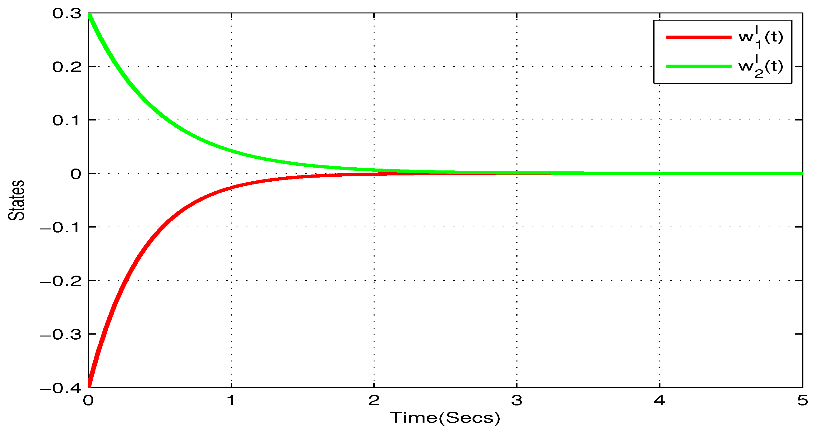
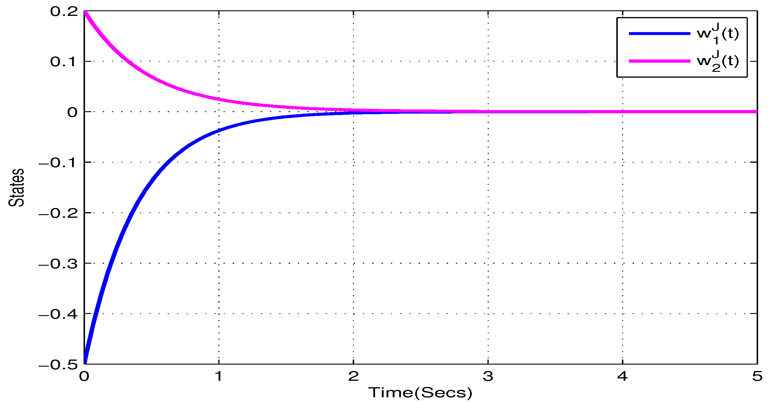
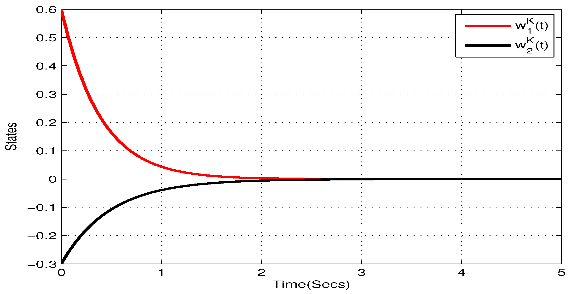
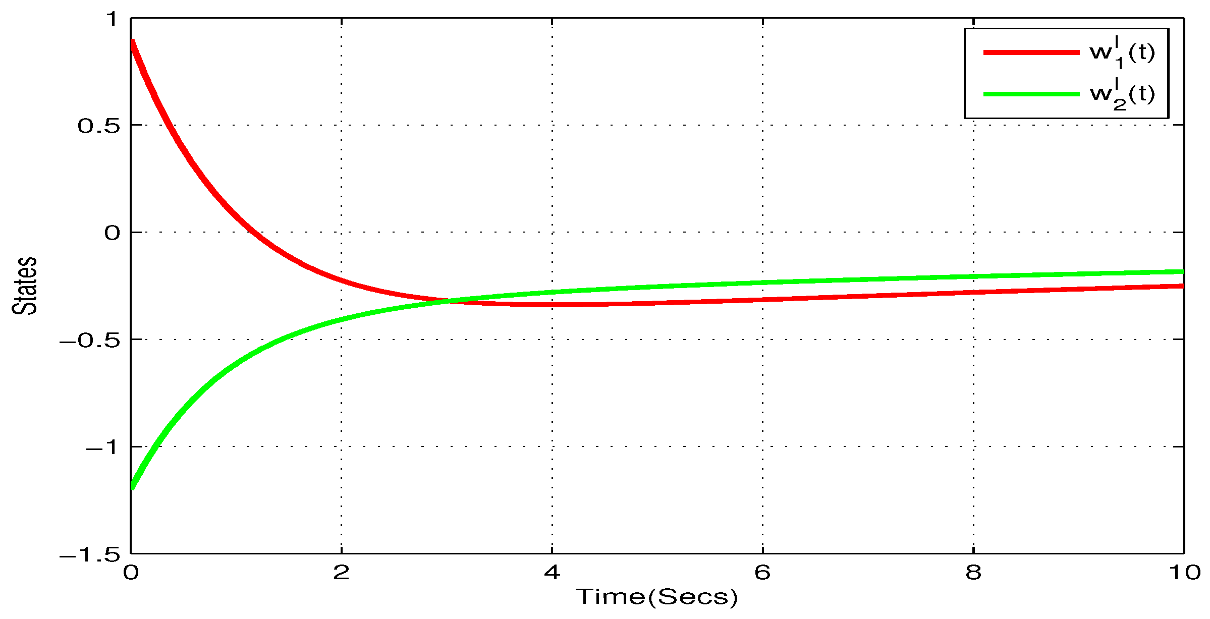
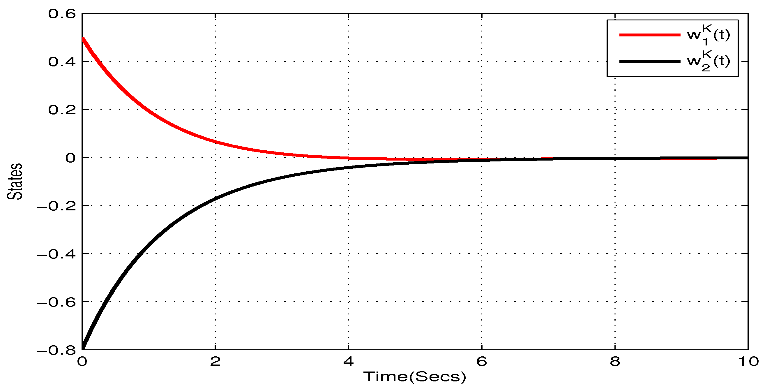
In addition, choose y R R = y I I = y J J = y K K = 1 , y R I = y R J = y R K = 0 , y I R = y I J = y I K = 0 , y J R = y J I = y J K = 0 , y K R = y K I = y K J = 0 , y = 1 , 2 . and ς = 2 , υ = 1 , = 1 , 2 , , 16 . According to Theorem 1, the NN (22) can realize global Mittag–Leffler stable. The initial values are taken as w 1 ( 0 ) = 0.3 + 0.4 i + 0.5 j 0.6 k and w 2 ( 0 ) = 0.1 0.3 i 0.2 j + 0.3 k . Figure 1, Figure 2, Figure 3 and Figure 4 show the state trajectory of NN (22). As plotted in Figure 1, Figure 2, Figure 3 and Figure 4, state trajectory of NN (22) converges to the equilibrium point.
Example 2.
Consider the following two-neurons FOQVMNNs:
D 0 , t σ C w 1 ( t ) = a 1 w 1 ( t ) + [ b 11 R ( w 1 ( t ) ) + b 11 I ( w 1 ( t ) ) + b 11 J ( w 1 ( t ) ) + b 11 K ( w 1 ( t ) ) ] g 1 ( w 1 ( t ) ) + [ b 12 R ( w 1 ( t ) ) + b 12 I ( w 1 ( t ) ) + b 12 J ( w 1 ( t ) ) + b 12 K ( w 1 ( t ) ) ] g 2 ( w 2 ( t ) ) + u 1 ( t ) D 0 , t σ C w 2 ( t ) = a 2 w 2 ( t ) + [ b 21 R ( w 2 ( t ) ) + b 21 I ( w 2 ( t ) ) + b 21 J ( w 2 ( t ) ) + b 21 K ( w 2 ( t ) ) ] g 1 ( w 1 ( t ) ) + [ b 22 R ( w 2 ( t ) ) + b 22 I ( w 2 ( t ) ) + b 22 J ( w 2 ( t ) ) + b 22 K ( w 2 ( t ) ) ] g 2 ( w 2 ( t ) ) + u 2 ( t ) ,
where σ = 0.98 , g x ( w x ( t ) ) = 0.5 t a n h ( w ( t ) ) , a 1 = 0.8 , a 2 = 1.2 , and
b 11 R ( w 1 ( t ) ) = 0.4 , | w 1 ( t ) | < 1 0.4 , | w 1 ( t ) | > 1 , b 11 I ( w 1 ( t ) ) = 0.4 , | w 1 ( t ) | < 1 0.4 , | w 1 ( t ) | > 1 , b 11 J ( w 1 ( t ) ) = 0.18 , | w 1 ( t ) | < 1 0.18 , | w 1 ( t ) | > 1 , b 11 K ( w 1 ( t ) ) = 0.6 , | w 1 ( t ) | < 1 0.6 , | w 1 ( t ) | > 1 , b 12 R ( w 1 ( t ) ) = 0.2 , | w 1 ( t ) | < 1 0.2 , | w 1 ( t ) | > 1 , b 12 I ( w 1 ( t ) ) = 0.5 , | w 1 ( t ) | < 1 0.5 , | w 1 ( t ) | > 1 , b 12 J ( w 1 ( t ) ) = 0.6 , | w 1 ( t ) | < 1 0.6 , | w 1 ( t ) | > 1 , b 12 K ( w 1 ( t ) ) = 0.7 , | w 1 ( t ) | < 1 0.7 , | w 1 ( t ) | > 1 , b 21 R ( w 2 ( t ) ) = 0.2 , | w 2 ( t ) | < 1 0.2 , | w 2 ( t ) | > 1 , b 21 I ( w 2 ( t ) ) = 0.12 , | w 2 ( t ) | < 1 0.12 , | w 2 ( t ) | > 1 , b 21 J ( w 2 ( t ) ) = 0.24 , | w 2 ( t ) | < 1 0.24 , | w 2 ( t ) | > 1 , b 21 K ( w 2 ( t ) ) = 0.35 , | w 2 ( t ) | < 1 0.35 , | w 2 ( t ) | > 1 , b 22 R ( w 2 ( t ) ) = 0.4 , | w 2 ( t ) | < 1 0.4 , | w 2 ( t ) | > 1 , b 22 I ( w 2 ( t ) ) = 0.24 , | w 2 ( t ) | < 1 0.24 , | w 2 ( t ) | > 1 , b 22 J ( w 2 ( t ) ) = 0.10 , | w 2 ( t ) | < 1 0.10 , | w 2 ( t ) | > 1 , b 22 K ( w 2 ( t ) ) = 0.20 , | w 2 ( t ) | < 1 0.20 , | w 2 ( t ) | > 1 .
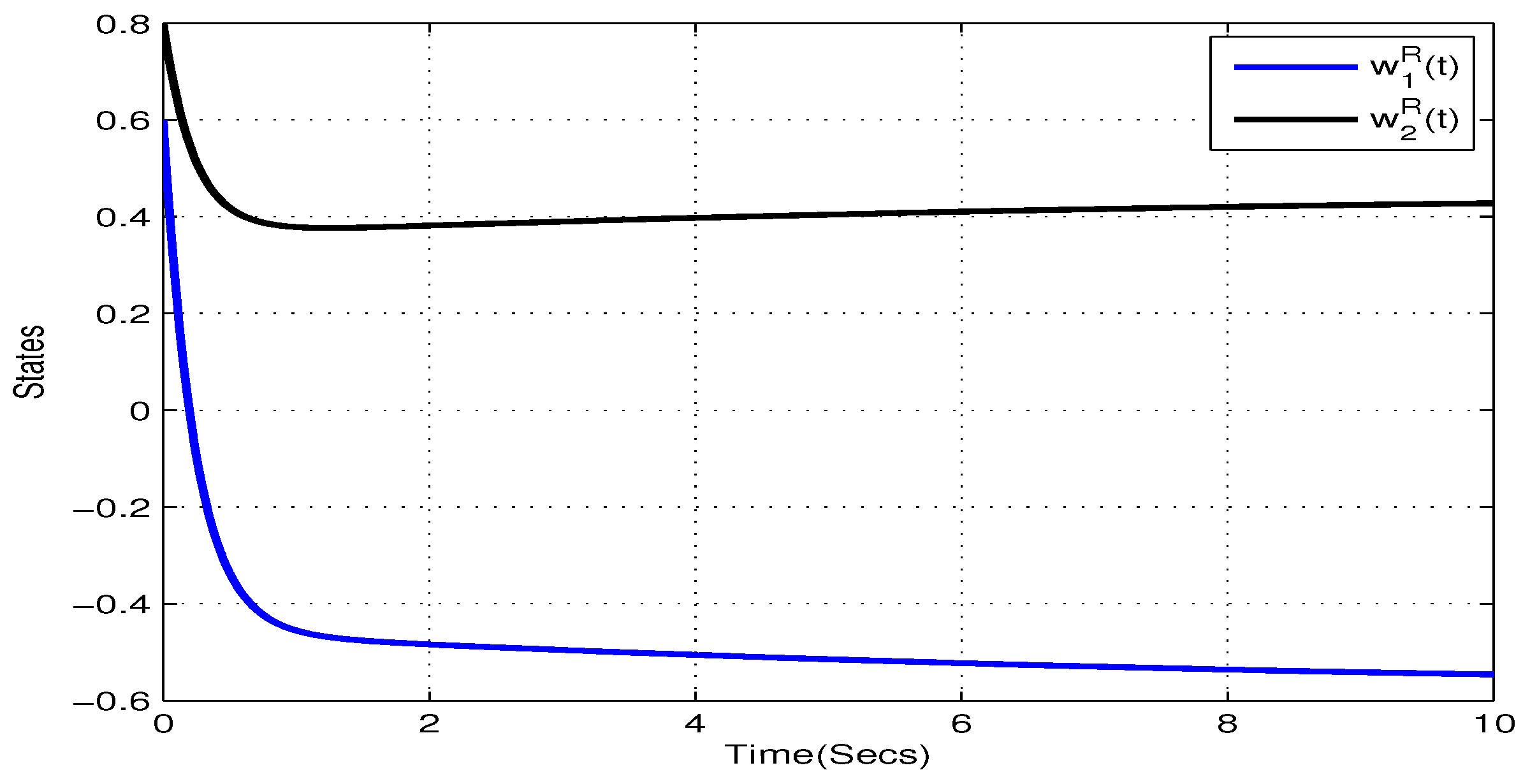
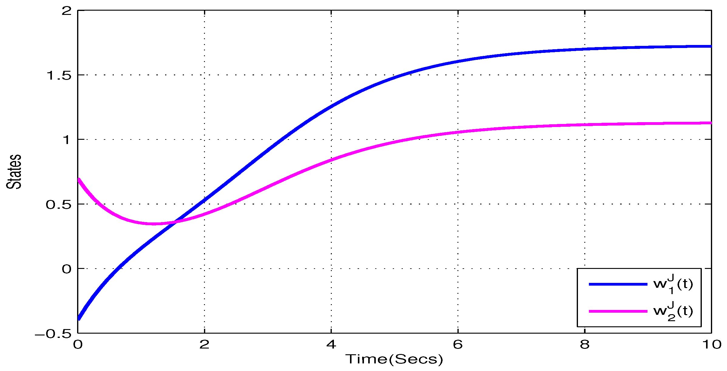
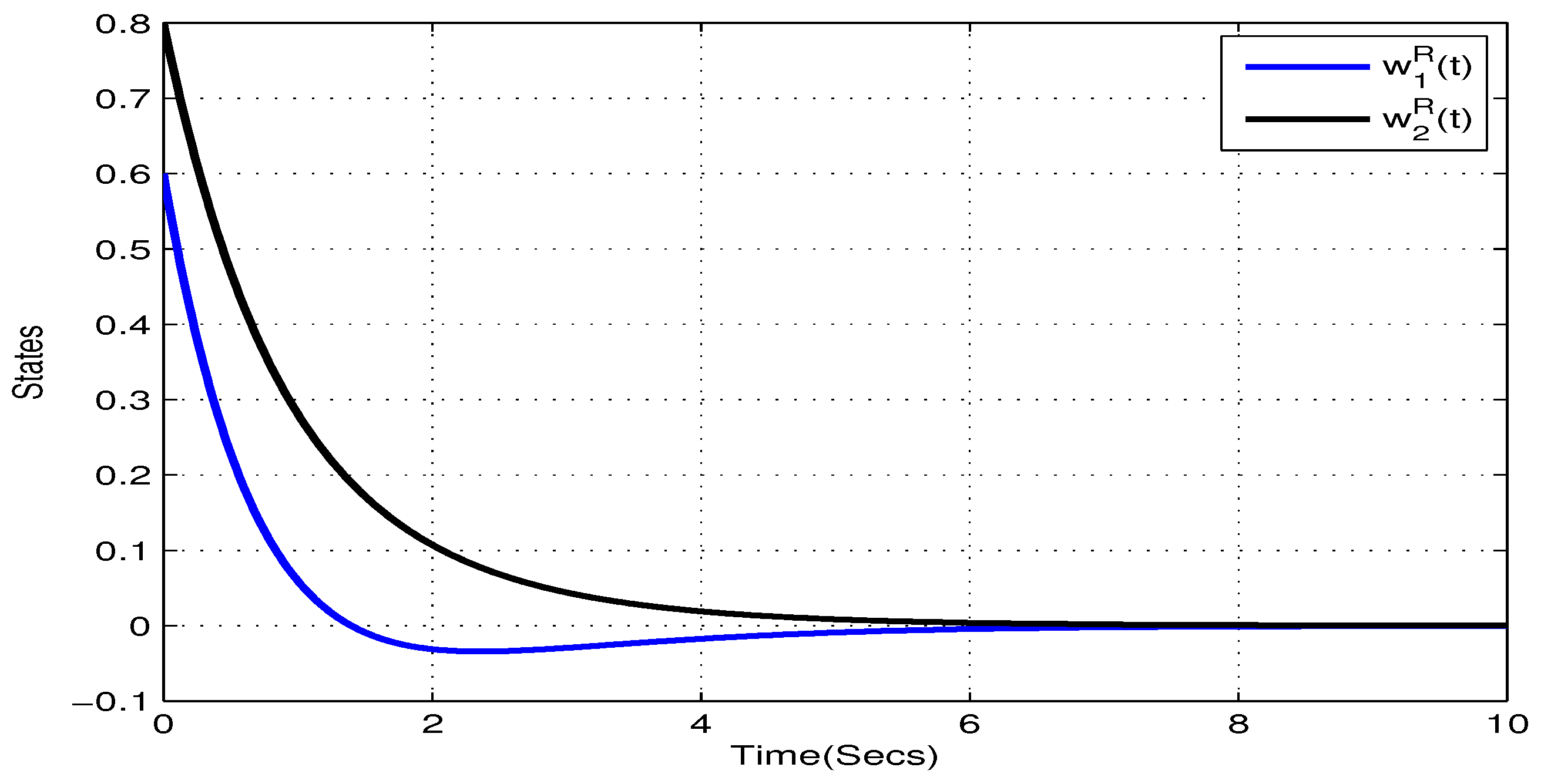
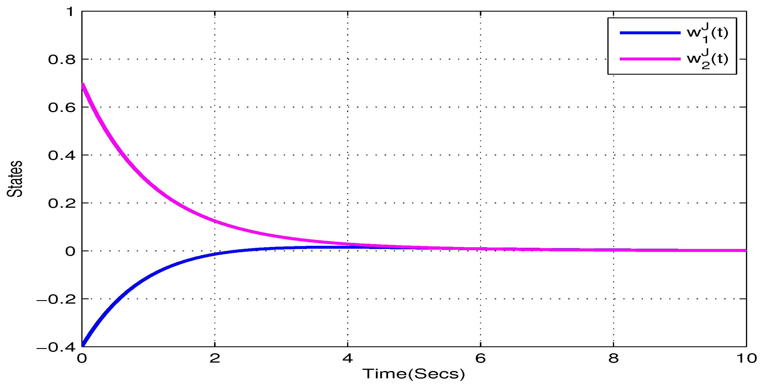
Take y R R = y I I = y J J = y K K = 1 , y R I = y R J = y R K = 0 , y I R = y I J = y I K = 0 , y J R = y J I = y J K = 0 , y K R = y K I = y K J = 0 , y = 1 , 2 . and ς = 2 , υ = 1 , = 1 , 2 , , 16 . Figure 5, Figure 6, Figure 7 and Figure 8 show the state trajectory of NN (23) without control input, respectively. As plotted in Figure 5, Figure 6, Figure 7 and Figure 8, state trajectory of NN (23) is divergent under the initial values w 1 ( 0 ) = 0.6 0.9 i + 0.4 j 0.5 k and w 2 ( 0 ) = 0.8 + 1.2 i 0.7 j 0.8 k . On the basis of above values, we can conclude | μ 1 | < 0.14 and | μ 2 | < 0.44 . According to Theorem 2, the NN (23) can realize global Mittag–Leffler stabilization when we choose the state feedback control law u 1 ( t ) = 0.14 w 1 ( t ) , u 2 ( t ) = 0.44 w 2 ( t ) . Figure 9 depicts the state trajectory of real parts of NN (23) with state feedback control law u 1 ( t ) = 0.12 a 1 ( t ) , u 2 ( t ) = 0.42 a 2 ( t ) . Similarly, Figure 10, Figure 11 and Figure 12 shows the state trajectory of imaginary parts of NN (23) with state feedback control law, respectively u 1 ( t ) = 0.12 b 1 ( t ) , u 2 ( t ) = 0.42 b 2 ( t ) , u 1 ( t ) = 0.12 c 1 ( t ) , u 2 ( t ) = 0.42 c 2 ( t ) , u 1 ( t ) = 0.12 d 1 ( t ) , u 2 ( t ) = 0.42 d 2 ( t ) .

5. Conclusions

This article dealt with the global Mittag–Leffler stability and stabilization analysis of FOQVMNNs. The state feedback stabilizing control law is designed to stabilize the considered NNs. To solve this problem easily, by applying Hamilton rules in quaternion multiplication, the FOQVMNN is divided into four fractional-order real-valued FOQVMNNs. By using the method of Lyapunov fractional-order derivative, fractional-order differential inclusions, set-valued maps, several global Mittag–Leffler stability, and stabilization conditions of considered FOQVMNNs are established. The feasibility and advantages of the results obtained are illustrated in two numerical examples. We wish to point out that our main results will lead to the generalization of more QVNNs such as discrete-time QVNNs, stochastic QVNNs, and uncertain QVNNs. In the near future, we will focus on the robust stability of discrete-time QVNNs.

Author Contributions

Funding acquisition, P.C.; Conceptualization, G.R.; Software, P.C., P.K. and R.S.; Formal analysis, G.R.; Methodology, G.R.; Supervision, C.P.L.; Writing—original draft, G.R.; Validation, G.R.; Writing—review and editing, G.R. All authors have read and agreed to the published version of the manuscript.

Funding

This research was supported by Chiang Mai University.

Acknowledgments

This research was supported by Chiang Mai University.

Conflicts of Interest

The authors declare no conflict of interest.

Appendix A

Proof. 
Proof of Theorem 1
We define the following Lyapunov function:
V ( w x ( t ) ) = x = 1 4 n 1 ς | w x ( t ) | ς = x = 1 n 1 ς | a x ( t ) | ς + x = 1 n 1 ς | b x ( t ) | ς + x = 1 n 1 ς | c x ( t ) | ς + x = 1 n 1 ς | d x ( t ) | ς .
From (7), it follows that
D 0 , t σ C V ( w x ( t ) ) x = 1 n | a x ( t ) | ς 1 [ a x | a x ( t ) | + y = 1 n α ˜ x y R | G y R | y = 1 n α ˜ x y I | G y I | y = 1 n α ˜ x y J | G y J | y = 1 n α ˜ x y K | G y K | ] + x = 1 n | b x ( t ) | ς 1 [ a x | b x ( t ) | + y = 1 n α ˜ x y R | G y I | + y = 1 n α ˜ x y I | G y R | + y = 1 n α ˜ x y J | G y K | y = 1 n α ˜ x y K | G y J | ] + x = 1 n | c x ( t ) | ς 1 [ a x | c x ( t ) | + y = 1 n α ˜ x y R | G y J | + y = 1 n α ˜ x y J | G y R | + y = 1 n α ˜ x y K | G y I | y = 1 n α ˜ x y I | G y K | ] + x = 1 n | d x ( t ) | ς 1 [ a x | d x ( t ) | + y = 1 n α ˜ x y R | G y K | + y = 1 n α ˜ x y I | G y I | + y = 1 n α ˜ x y K | G y R | y = 1 n α ˜ x y J | G y I | ,
D 0 , t σ C V ( w x ( t ) ) x = 1 n | a x ( t ) | ς 1 [ a x | a x ( t ) | + y = 1 n α ˜ x y R ( G y * ) y = 1 n α ˜ x y I ( G y * * ) y = 1 n α ˜ x y J ( G y * * * ) y = 1 n α ˜ x y K ( G y * * * * ) ] + x = 1 n | b x ( t ) | ς 1 [ a x | b x ( t ) | + y = 1 n α ˜ x y R ( G y * * ) + y = 1 n α ˜ x y I ( G y * ) + y = 1 n α ˜ x y J ( G y * * * * ) y = 1 n α ˜ x y K ( G y * * * ) ] + x = 1 n | c x ( t ) | ς 1 [ a x | c x ( t ) | + y = 1 n α ˜ x y R ( G y * * * ) + y = 1 n α ˜ x y J ( G y * ) + y = 1 n α ˜ x y K ( G y * * ) y = 1 n α ˜ x y I ( G y * * * * ) ] + x = 1 n | d x ( t ) | ς 1 [ a x | d x ( t ) | + y = 1 n α ˜ x y R ( G y * * * * ) + y = 1 n α ˜ x y I ( G y * * * ) + y = 1 n α ˜ x y K ( G y * ) y = 1 n α ˜ x y J ( G y * * ) ,
D 0 , t σ C V ( w x ( t ) ) x = 1 n a x | a x ( t ) | ς + x = 1 n y = 1 n α ˜ x y R y R R | a x | * | a y | + x = 1 n y = 1 n α ˜ x y R y R I | a x | * | b y | + x = 1 n y = 1 n α ˜ x y R y R J | a x | * | c y | + x = 1 n y = 1 n α ˜ x y R y R K | a x | * | d y | x = 1 n y = 1 n α ˜ x y I y I R | a x | * | a y | x = 1 n y = 1 n α ˜ x y I y I I | a x | * | b y | x = 1 n y = 1 n α ˜ x y I y I J | a x ( t ) | a x | * | c y | x = 1 n y = 1 n α ˜ x y I y I K | a x | * | d y | x = 1 n y = 1 n α ˜ x y J y J R | a x | * | a y | x = 1 n y = 1 n α ˜ x y J y J I | a x | * | b y | x = 1 n y = 1 n α ˜ x y J y J J | a x | * | c y | x = 1 n y = 1 n α ˜ x y J y J K | a x | * | d y | x = 1 n y = 1 n α ˜ x y K y K R | a x | * | a y | x = 1 n y = 1 n α ˜ x y K y K I | a x | * | b y | x = 1 n y = 1 n α ˜ x y K y K J | a x | * | c y | x = 1 n y = 1 n α ˜ x y K y K K | a x | * | d y | x = 1 n a x | a x | * | a y | | b x ( t ) | ς + x = 1 n y = 1 n α ˜ x y R y I R | b x | * | a y | + x = 1 n y = 1 n α ˜ x y R y I I | b x | * | b y | + x = 1 n y = 1 n α ˜ x y R y I J | b x | * | c y | + x = 1 n y = 1 n α ˜ x y R y I K | b x | * | d y | + x = 1 n y = 1 n α ˜ x y I y R R | b x | * | a y | + x = 1 n y = 1 n α ˜ x y I y R I | b x | * | b y | + x = 1 n y = 1 n α ˜ x y I y R J | b x | * | c y | + x = 1 n y = 1 n α ˜ x y I y R K | b x | * | d y | + x = 1 n y = 1 n α ˜ x y J y K R | b x | * | a y | + x = 1 n y = 1 n α ˜ x y J y K I | b x | * | b y | + x = 1 n y = 1 n α ˜ x y J y K J | b x | * | c y | + x = 1 n y = 1 n α ˜ x y J y K K | b x | * | d y | x = 1 n y = 1 n α ˜ x y K y J R | b x | * | a y | x = 1 n y = 1 n α ˜ x y K y J I | b x | * | b y | x = 1 n y = 1 n α ˜ x y K y J J | b x | * | c y | x = 1 n y = 1 n α ˜ x y K y J K | b x | * | d y | x = 1 n a x | c x ( t ) | ς + x = 1 n y = 1 n α ˜ x y R y J R | c x | * | a y | + x = 1 n y = 1 n α ˜ x y R y J I | c x | * | b y | + x = 1 n y = 1 n α ˜ x y R y J J | c x | * | c y | + x = 1 n y = 1 n α ˜ x y R y J K | c x | * | d y | + x = 1 n y = 1 n α ˜ x y J y R R | c x | * | a y | + x = 1 n y = 1 n α ˜ x y J y R I | c x | * | b y | + x = 1 n y = 1 n α ˜ x y J y R J | c x | * | c y | + x = 1 n y = 1 n α ˜ x y J y R K | c x | * | d y | + x = 1 n y = 1 n α ˜ x y K y I R | c x | * | a y | + x = 1 n y = 1 n α ˜ x y K y I I | c x | * | b y | + x = 1 n y = 1 n α ˜ x y K y I J | c x | * | c y | + x = 1 n y = 1 n α ˜ x y K y I K | c x | * | d y | x = 1 n y = 1 n α ˜ x y I y K R | c x | * | a y | x = 1 n y = 1 n α ˜ x y I y K I | c x | * | b y | x = 1 n y = 1 n α ˜ x y I y K J | c x | * | c y | x = 1 n y = 1 n α ˜ x y I y K K | c x | * | d y | x = 1 n x = 1 n a x | d x ( t ) | ς + x = 1 n y = 1 n α ˜ x y R y K R | d x | * | a y | + x = 1 n y = 1 n α ˜ x y R y K I | d x | * | b y | + x = 1 n y = 1 n α ˜ x y R y K J | d x | * | c y | + x = 1 n y = 1 n α ˜ x y R y K K | d x | * | d y | + x = 1 n y = 1 n α ˜ x y I y J R | d x | * | a y | + x = 1 n y = 1 n α ˜ x y I y J I | d x | * | b y | + x = 1 n y = 1 n α ˜ x y I y J J | d x | * | c y | + x = 1 n y = 1 n α ˜ x y I y J K | d x | * | d y | + x = 1 n y = 1 n α ˜ x y K y R R | d x | * | a y | + x = 1 n y = 1 n α ˜ x y K y R I | d x | * | b y | + x = 1 n y = 1 n α ˜ x y K y R J | d x | * | c y | + x = 1 n y = 1 n α ˜ x y K y R K | d x | * | d y | x = 1 n y = 1 n α ˜ x y J y I R | d x | * | a y | x = 1 n y = 1 n α ˜ x y J y I I | d x | * | b y | x = 1 n y = 1 n α ˜ x y J y I J | d x | * | c y | x = 1 n y = 1 n α ˜ x y J y I K | d x | * | d y .
By Lemma 1, it follows that
| a x | * | a y | ς 1 ς [ | a x ( t ) | ς 1 υ 1 ς 1 ς ] ς ς 1 + 1 ς [ | a y ( t ) | υ 1 ς 1 ς ] ς = | a * a | y .
In the same way, we have
| a x | * | b y | | a * b | y ,
| a x | * | c y | | a * c | y ,
| a x | * | d y | | a * d | y ,
| b x | * | a y | | b * a | y ,
| b x | * | b y | | b * b | y ,
| b x | * | c y | | b * c | y ,
| b x | * | d y | | b * d | y ,
| c x | * | a y | | c * a | y ,
| c x | * | b y | | c * b | y ,
| c x | * | c y | | c * c | y ,
| c x | * | d y | | c * d | y ,
| d x | * | a y | | d * a | y ,
| d x | * | b y | | d * b | y ,
| d x | * | c y | | d * c | y ,
| d x | * | d y | | d * d | y .
Substituting (A5)–(A20) into (A4), then
D 0 , t σ C V ( w x ( t ) ) x = 1 n a x | a x ( t ) | ς + x = 1 n y = 1 n α ˜ x y R y R R | a * a | y + x = 1 n y = 1 n α ˜ x y R y R I | a * b | y + x = 1 n y = 1 n α ˜ x y R y R J | a * c | y + x = 1 n y = 1 n α ˜ x y R y R K | a * d | y x = 1 n y = 1 n α ˜ x y I y I R | a * a | y x = 1 n y = 1 n α ˜ x y I y I I | a * b | y x = 1 n y = 1 n α ˜ x y I y I J | a * c | y x = 1 n y = 1 n α ˜ x y I y I K | a * d | y x = 1 n y = 1 n α ˜ x y J y J R | a * a | y x = 1 n y = 1 n α ˜ x y J y J I | a * b | y x = 1 n y = 1 n α ˜ x y J y J J | a * c | y x = 1 n y = 1 n α ˜ x y J y J K | a * d | y x = 1 n y = 1 n α ˜ x y K y K R | a * a | y x = 1 n y = 1 n α ˜ x y K y K I | a * b | y x = 1 n y = 1 n α ˜ x y K y K J | a * c | y x = 1 n y = 1 n α ˜ x y K y K K | a * d | y x = 1 n a x | b x ( t ) | ς + x = 1 n y = 1 n α ˜ x y R y I R | b * a | y + x = 1 n y = 1 n α ˜ x y R y I I | b * b | y + x = 1 n y = 1 n α ˜ x y R y I J | b * c | y + x = 1 n y = 1 n α ˜ x y R y I K | b * d | y + x = 1 n y = 1 n α ˜ x y I y R R | b * a | y + x = 1 n y = 1 n α ˜ x y I y R I | b * b | y + x = 1 n y = 1 n α ˜ x y I y R J | b * c | y + x = 1 n y = 1 n α ˜ x y I y R K | b * d | y + x = 1 n y = 1 n α ˜ x y J y K R | b * a | y + x = 1 n y = 1 n α ˜ x y J y K I | b * b | y + x = 1 n y = 1 n α ˜ x y J y K J | b * c | y + x = 1 n y = 1 n α ˜ x y J y K K | b * d | y x = 1 n y = 1 n α ˜ x y K y J R | b * a | y x = 1 n y = 1 n α ˜ x y K y J I | b * b | y x = 1 n y = 1 n α ˜ x y K y J J | b * c | y x = 1 n y = 1 n α ˜ x y K y J K | b * d | y x = 1 n a x | c x ( t ) | ς + x = 1 n y = 1 n α ˜ x y R y J R | b * a | y + x = 1 n y = 1 n α ˜ x y R y J I | b * b | y + x = 1 n y = 1 n α ˜ x y R y J J | b * c | y + x = 1 n y = 1 n α ˜ x y R y J K | b * d | y + x = 1 n y = 1 n α ˜ x y J y R R | b * a | y + x = 1 n y = 1 n α ˜ x y J y R I | b * b | y + x = 1 n y = 1 n α ˜ x y J y R J | b * c | y + x = 1 n y = 1 n α ˜ x y J y R K | b * d | y + x = 1 n y = 1 n α ˜ x y K y I R | c * a | y + x = 1 n y = 1 n α ˜ x y K y I I | c * b | y + x = 1 n y = 1 n α ˜ x y K y I J | c * c | y + x = 1 n y = 1 n α ˜ x y K y I K | c * d | y x = 1 n y = 1 n α ˜ x y I y K R | c * a | y x = 1 n y = 1 n α ˜ x y I y K I | c * b | y x = 1 n y = 1 n α ˜ x y I y K J | c * c | y x = 1 n y = 1 n α ˜ x y I y K K | c * d | y x = 1 n x = 1 n a x | d x ( t ) | ς + x = 1 n y = 1 n α ˜ x y R y K R | d * a | y + x = 1 n y = 1 n α ˜ x y R y K I | d * b | y + x = 1 n y = 1 n α ˜ x y R y K J | d * c | y + x = 1 n y = 1 n α ˜ x y R y K K | d * d | y + x = 1 n y = 1 n α ˜ x y I y J R | d * a | y + x = 1 n y = 1 n α ˜ x y I y J I | d * b | y + x = 1 n y = 1 n α ˜ x y I y J J | d * c | y + x = 1 n y = 1 n α ˜ x y I y J K | d * d | y + x = 1 n y = 1 n α ˜ x y K y R R | d * a | y + x = 1 n y = 1 n α ˜ x y K y R I | d * b | y + x = 1 n y = 1 n α ˜ x y K y R J | d * c | y + x = 1 n y = 1 n α ˜ x y K y R K | d * d | y x = 1 n y = 1 n α ˜ x y J y I R | d * a | y x = 1 n y = 1 n α ˜ x y J y I I | d * b | y x = 1 n y = 1 n α ˜ x y J y I J | d * c | y x = 1 n y = 1 n α ˜ x y J y I K | d * d | y .
= x = 1 n { a x ς + y = 1 n α ˜ x y R y R R ( ς 1 ) υ 1 + y = 1 n α ˜ y x R x R R 1 υ 1 ς 1 + y = 1 n α ˜ x y R y R I ( ς 1 ) υ 2 + y = 1 n α ˜ x y R y R J ( ς 1 ) υ 3 + y = 1 n α ˜ x y R y R K ( ς 1 ) υ 4 y = 1 n α ˜ x y I y I R ( ς 1 ) υ 1 y = 1 n α ˜ y x I x I R 1 υ 1 ς 1 y = 1 n α ˜ x y I y I I ( ς 1 ) υ 2 y = 1 n α ˜ x y I y I J ( ς 1 ) υ 3 y = 1 n α ˜ x y I y I K ( ς 1 ) υ 4 y = 1 n α ˜ x y J y J R ( ς 1 ) υ 1 y = 1 n α ˜ y x J x J R 1 υ 1 ς 1 y = 1 n α ˜ x y J y J I ( ς 1 ) υ 2 y = 1 n α ˜ x y J y J J ( ς 1 ) υ 3 y = 1 n α ˜ x y J y J K ( ς 1 ) υ 4 y = 1 n α ˜ x y K y K R ( ς 1 ) υ 1 y = 1 n α ˜ y x K x K R 1 υ 1 ς 1 y = 1 n α ˜ x y K y K I ( ς 1 ) υ 2 y = 1 n α ˜ x y K y K J ( ς 1 ) υ 3 y = 1 n α ˜ x y K y K K ( ς 1 ) υ 4 + y = 1 n α ˜ y x R x I R 1 υ 5 ς 1 + y = 1 n α ˜ y x I x R R 1 υ 5 ς 1 + y = 1 n α ˜ y x J x K R 1 υ 5 ς 1 y = 1 n α ˜ y x K x J R 1 υ 5 ς 1 + y = 1 n α ˜ y x R x J R 1 υ 9 ς 1 + y = 1 n α ˜ y x J x R R 1 υ 9 ς 1 + y = 1 n α ˜ y x K x I R 1 υ 9 ς 1 y = 1 n α ˜ y x I x K R 1 υ 9 ς 1 + y = 1 n α ˜ y x R x K R 1 υ 13 ς 1 + y = 1 n α ˜ y x I x J R 1 υ 13 ς 1 + y = 1 n α ˜ y x K x R R 1 υ 13 ς 1 y = 1 n α ˜ y x J x I R 1 υ 13 ς 1 } | a x ( t ) | ς ς + x = 1 n { a x ς + y = 1 n α ˜ y x R x R I 1 υ 2 ς 1 y = 1 n α ˜ y x I x I I 1 υ 2 ς 1 y = 1 n α ˜ y x J x J I 1 υ 2 ς 1 y = 1 n α ˜ y x K x K I 1 υ 2 ς 1 + y = 1 n α ˜ x y R y I R ( ς 1 ) υ 5 + y = 1 n α ˜ x y R y I I ( ς 1 ) υ 6 + y = 1 n α ˜ y x R x I I 1 υ 6 ς 1 + y = 1 n α ˜ x y R y I J ( ς 1 ) υ 7 + y = 1 n α ˜ x y R y I K ( ς 1 ) υ 8 + y = 1 n α ˜ x y I y R R ( ς 1 ) υ 5 + y = 1 n α ˜ x y I y R I ( ς 1 ) υ 6 + y = 1 n α ˜ y x I x R I 1 υ 6 ς 1 + y = 1 n α ˜ x y I y R J ( ς 1 ) υ 7 + y = 1 n α ˜ x y I y R K ( ς 1 ) υ 8 + y = 1 n α ˜ x y J y K R ( ς 1 ) υ 5 + y = 1 n α ˜ x y I y R I ( ς 1 ) υ 6 + y = 1 n α ˜ y x J x K I 1 υ 6 ς 1 + y = 1 n α ˜ x y J y K J ( ς 1 ) υ 7 + y = 1 n α ˜ x y J y K K ( ς 1 ) υ 8 y = 1 n α ˜ x y K y J R ( ς 1 ) υ 5 y = 1 n α ˜ x y K y J I ( ς 1 ) υ 6 y = 1 n α ˜ y x K x J I 1 υ 6 ς 1 y = 1 n α ˜ x y K y J J ( ς 1 ) υ 7 y = 1 n α ˜ x y K y J K ( ς 1 ) υ 8 + y = 1 n α ˜ y x R x J I 1 υ 10 ς 1 + y = 1 n α ˜ y x J x R I 1 υ 10 ς 1 + y = 1 n α ˜ y x K x I I 1 υ 10 ς 1 y = 1 n α ˜ y x I x K I 1 υ 10 ς 1 + y = 1 n α ˜ y x R x K I 1 υ 14 ς 1 + y = 1 n α ˜ y x I x J I 1 υ 14 ς 1 + y = 1 n α ˜ y x K x R I 1 υ 14 ς 1 + y = 1 n α ˜ y x J x I I 1 υ 14 ς 1 } | b x ( t ) | ς ς + x = 1 n { a x ς + y = 1 n α ˜ y x R x R J 1 υ 3 ς 1 y = 1 n α ˜ y x I x I J 1 υ 3 ς 1 y = 1 n α ˜ y x J x J J 1 υ 3 ς 1 y = 1 n α ˜ y x K x K J 1 υ 3 ς 1 + y = 1 n α ˜ y x R x I J 1 υ 7 ς 1 + y = 1 n α ˜ y x I x R J 1 υ 7 ς 1 + y = 1 n α ˜ y x J x K J 1 υ 7 ς 1 y = 1 n α ˜ y x K x J J 1 υ 7 ς 1 + y = 1 n α ˜ x y R y J R ( ς 1 ) υ 9 + y = 1 n α ˜ x y R y J I ( ς 1 ) υ 10 + y = 1 n α ˜ x y R y J J ( ς 1 ) υ 11 + y = 1 n α ˜ y x R x J J 1 υ 11 ς 1 + y = 1 n α ˜ x y R y J K ( ς 1 ) υ 12 + y = 1 n α ˜ x y J y R R ( ς 1 ) υ 9 + y = 1 n α ˜ x y J y R I ( ς 1 ) υ 10 + y = 1 n α ˜ x y J y R J ( ς 1 ) υ 11 + y = 1 n α ˜ y x J x R J 1 υ 11 ς 1 + y = 1 n α ˜ x y J y R K ( ς 1 ) υ 12 + y = 1 n α ˜ x y K y I R ( ς 1 ) υ 9 + y = 1 n α ˜ x y K y I I ( ς 1 ) υ 10 + y = 1 n α ˜ x y K y I J ( ς 1 ) υ 11 + y = 1 n α ˜ y x K x I J 1 υ 11 ς 1 + y = 1 n α ˜ x y K y I K ( ς 1 ) υ 12 y = 1 n α ˜ x y I y K R ( ς 1 ) υ 9 y = 1 n α ˜ x y I y K I ( ς 1 ) υ 10 y = 1 n α ˜ x y I y K J ( ς 1 ) υ 11 y = 1 n α ˜ y x I x K J 1 υ 11 ς 1 y = 1 n α ˜ x y I y K K ( ς 1 ) υ 12 + y = 1 n α ˜ y x R x K J 1 υ 15 ς 1 + y = 1 n α ˜ y x I x J J 1 υ 15 ς 1 + y = 1 n α ˜ y x K x R J 1 υ 15 ς 1 y = 1 n α ˜ y x J x I J 1 υ 15 ς 1 } | c x ( t ) | ς ς + x = 1 n { a x ς + y = 1 n α ˜ y x R x R K 1 υ 4 ς 1 y = 1 n α ˜ y x I x I K 1 υ 4 ς 1 y = 1 n α ˜ y x J x J K 1 υ 4 ς 1 y = 1 n α ˜ y x K x K K 1 υ 4 ς 1 + y = 1 n α ˜ y x R x I K 1 υ 8 ς 1 + y = 1 n α ˜ y x I x R K 1 υ 8 ς 1 + y = 1 n α ˜ y x J x K K 1 υ 8 ς 1 y = 1 n α ˜ y x K x J K 1 υ 8 ς 1 + y = 1 n α ˜ y x R x J K 1 υ 12 ς 1 + y = 1 n α ˜ y x J x R K 1 υ 12 ς 1 + y = 1 n α ˜ y x K x I K 1 υ 12 ς 1 y = 1 n α ˜ y x I x K K 1 υ 12 ς 1 + y = 1 n α ˜ x y R y K R ( ς 1 ) υ 13 + y = 1 n α ˜ x y R y K I ( ς 1 ) υ 14 + y = 1 n α ˜ x y R y K J ( ς 1 ) υ 15 + y = 1 n α ˜ x y R y K K ( ς 1 ) υ 16 + y = 1 n α ˜ y x R x K K 1 υ 16 ς 1 + y = 1 n α ˜ x y I y J R ( ς 1 ) υ 13 + y = 1 n α ˜ x y I y J I ( ς 1 ) υ 14 + y = 1 n α ˜ x y I y J J ( ς 1 ) υ 15 + y = 1 n α ˜ x y I y J K ( ς 1 ) υ 16 + y = 1 n α ˜ y x I x J K 1 υ 16 ς 1 + y = 1 n α ˜ x y K y R R ( ς 1 ) υ 13 + y = 1 n α ˜ x y K y R I ( ς 1 ) υ 14 + y = 1 n α ˜ x y K y R J ( ς 1 ) υ 15 + y = 1 n α ˜ x y K y R K ( ς 1 ) υ 16 + y = 1 n α ˜ y x K x R K 1 υ 16 ς 1 y = 1 n α ˜ x y J y I R ( ς 1 ) υ 13 y = 1 n α ˜ x y J y I I ( ς 1 ) υ 14 y = 1 n α ˜ x y J y I J ( ς 1 ) υ 15 y = 1 n α ˜ x y J y I K ( ς 1 ) υ 16 y = 1 n α ˜ y x J x I K 1 υ 16 ς 1 } | d x ( t ) | ς ς C D 0 , t σ V ( w x ( t ) ) min 1 x 1 { a x ς y = 1 n α ˜ x y R y R R ( ς 1 ) υ 1 y = 1 n α ˜ y x R x R R 1 υ 1 ς 1 y = 1 n α ˜ x y R y R I ( ς 1 ) υ 2 y = 1 n α ˜ x y R y R J ( ς 1 ) υ 3 y = 1 n α ˜ x y R y R K ( ς 1 ) υ 4 + y = 1 n α ˜ x y I y I R ( ς 1 ) υ 1 + y = 1 n α ˜ y x I x I R 1 υ 1 ς 1 + y = 1 n α ˜ x y I y I I ( ς 1 ) υ 2 + y = 1 n α ˜ x y I y I J ( ς 1 ) υ 3 + y = 1 n α ˜ x y I y I K ( ς 1 ) υ 4 + y = 1 n α ˜ x y J y J R ( ς 1 ) υ 1 + y = 1 n α ˜ y x J x J R 1 υ 1 ς 1 + y = 1 n α ˜ x y J y J I ( ς 1 ) υ 2 + y = 1 n α ˜ x y J y J J ( ς 1 ) υ 3 + y = 1 n α ˜ x y J y J K ( ς 1 ) υ 4 + y = 1 n α ˜ x y K y K R ( ς 1 ) υ 1 y = 1 n α ˜ y x K x K R 1 υ 1 ς 1 + y = 1 n α ˜ x y K y K I ( ς 1 ) υ 2 + y = 1 n α ˜ x y K y K J ( ς 1 ) υ 3 + y = 1 n α ˜ x y K y K K ( ς 1 ) υ 4 y = 1 n α ˜ y x R x I R 1 υ 5 ς 1 y = 1 n α ˜ y x I x R R 1 υ 5 ς 1 y = 1 n α ˜ y x J x K R 1 υ 5 ς 1 + y = 1 n α ˜ y x K x J R 1 υ 5 ς 1 y = 1 n α ˜ y x R x J R 1 υ 9 ς 1 y = 1 n α ˜ y x J x R R 1 υ 9 ς 1 y = 1 n α ˜ y x K x I R 1 υ 9 ς 1 + y = 1 n α ˜ y x I x K R 1 υ 9 ς 1 y = 1 n α ˜ y x R x K R 1 υ 13 ς 1 y = 1 n α ˜ y x I x J R 1 υ 13 ς 1 y = 1 n α ˜ y x K x R R 1 υ 13 ς 1 + y = 1 n α ˜ y x J x I R 1 υ 13 ς 1 } x = 1 n | a x ( t ) | ς ς min 1 x 1 { a x ς y = 1 n α ˜ y x R x R I 1 υ 2 ς 1 + y = 1 n α ˜ y x I x I I 1 υ 2 ς 1 + y = 1 n α ˜ y x J x J I 1 υ 2 ς 1 + y = 1 n α ˜ y x K x K I 1 υ 2 ς 1 y = 1 n α ˜ x y R y I R ( ς 1 ) υ 5 y = 1 n α ˜ x y R y I I ( ς 1 ) υ 6 y = 1 n α ˜ y x R x I I 1 υ 6 ς 1 y = 1 n α ˜ x y R y I J ( ς 1 ) υ 7 y = 1 n α ˜ x y R y I K ( ς 1 ) υ 8 y = 1 n α ˜ x y I y R R ( ς 1 ) υ 5 y = 1 n α ˜ x y I y R I ( ς 1 ) υ 6 y = 1 n α ˜ y x I x R I 1 υ 6 ς 1 y = 1 n α ˜ x y I y R J ( ς 1 ) υ 7 y = 1 n α ˜ x y I y R K ( ς 1 ) υ 8 y = 1 n α ˜ x y J y K R ( ς 1 ) υ 5 y = 1 n α ˜ x y J y K I ( ς 1 ) υ 6 y = 1 n α ˜ y x J x K I 1 υ 6 ς 1 y = 1 n α ˜ x y J y K J ( ς 1 ) υ 7 y = 1 n α ˜ x y J y K K ( ς 1 ) υ 8 + y = 1 n α ˜ x y K y J R ( ς 1 ) υ 5 + y = 1 n α ˜ x y K y J I ( ς 1 ) υ 6 + y = 1 n α ˜ y x K x J I 1 υ 6 ς 1 + y = 1 n α ˜ x y K y J J ( ς 1 ) υ 7 + y = 1 n α ˜ x y K y J K ( ς 1 ) υ 8 y = 1 n α ˜ y x R x J I 1 υ 10 ς 1 y = 1 n α ˜ y x J x R I 1 υ 10 ς 1 y = 1 n α ˜ y x K x I I 1 υ 10 ς 1 + y = 1 n α ˜ y x I x K I 1 υ 10 ς 1 y = 1 n α ˜ y x R x K I 1 υ 14 ς 1 y = 1 n α ˜ y x I x J I 1 υ 14 ς 1 y = 1 n α ˜ y x K x R I 1 υ 14 ς 1 + y = 1 n α ˜ y x J x I I 1 υ 14 ς 1 } x = 1 n | b x ( t ) | ς ς min 1 x 1 { a x ς y = 1 n α ˜ y x R x R J 1 υ 3 ς 1 + y = 1 n α ˜ y x I x I J 1 υ 3 ς 1 + y = 1 n α ˜ y x J x J J 1 υ 3 ς 1 + y = 1 n α ˜ y x K x K J 1 υ 3 ς 1 y = 1 n α ˜ y x R x I J 1 υ 7 ς 1 y = 1 n α ˜ y x I x R J 1 υ 7 ς 1 y = 1 n α ˜ y x J x K J 1 υ 7 ς 1 + y = 1 n α ˜ y x K x J J 1 υ 7 ς 1 y = 1 n α ˜ x y R y J R ( ς 1 ) υ 9 y = 1 n α ˜ x y R y J I ( ς 1 ) υ 10 y = 1 n α ˜ x y R y J J ( ς 1 ) υ 11 y = 1 n α ˜ y x R x J J 1 υ 11 ς 1 y = 1 n α ˜ x y R y J K ( ς 1 ) υ 12 y = 1 n α ˜ x y J y R R ( ς 1 ) υ 9 y = 1 n α ˜ x y J y R I ( ς 1 ) υ 10 y = 1 n α ˜ x y J y R J ( ς 1 ) υ 11 y = 1 n α ˜ y x J x R J 1 υ 11 ς 1 y = 1 n α ˜ x y J y R K ( ς 1 ) υ 12 y = 1 n α ˜ x y K y I R ( ς 1 ) υ 9 y = 1 n α ˜ x y K y I I ( ς 1 ) υ 10 y = 1 n α ˜ x y K y I J ( ς 1 ) υ 11 y = 1 n α ˜ y x K x I J 1 υ 11 ς 1 y = 1 n α ˜ x y K y I K ( ς 1 ) υ 12 + y = 1 n α ˜ x y I y K R ( ς 1 ) υ 9 + y = 1 n α ˜ x y I y K I ( ς 1 ) υ 10 + y = 1 n α ˜ x y I y K J ( ς 1 ) υ 11 + y = 1 n α ˜ y x I x K J 1 υ 11 ς 1 + y = 1 n α ˜ x y I y K K ( ς 1 ) υ 12 y = 1 n α ˜ y x R x K J 1 υ 15 ς 1 y = 1 n α ˜ y x I x J J 1 υ 15 ς 1 y = 1 n α ˜ y x K x R J 1 υ 15 ς 1 + y = 1 n α ˜ y x J x I J 1 υ 15 ς 1 } x = 1 n | c x ( t ) | ς ς min 1 x 1 { a x ς y = 1 n α ˜ y x R x R K 1 υ 4 ς 1 + y = 1 n α ˜ y x I x I K 1 υ 4 ς 1 + y = 1 n α ˜ y x J x J K 1 υ 4 ς 1 + y = 1 n α ˜ y x K x K K 1 υ 4 ς 1 y = 1 n α ˜ y x R x I K 1 υ 8 ς 1 y = 1 n α ˜ y x I x R K 1 υ 8 ς 1 y = 1 n α ˜ y x J x K K 1 υ 8 ς 1 + y = 1 n α ˜ y x K x J K 1 υ 8 ς 1 y = 1 n α ˜ y x R x J K 1 υ 12 ς 1 y = 1 n α ˜ y x J x R K 1 υ 12 ς 1 y = 1 n α ˜ y x K x I K 1 υ 12 ς 1 + y = 1 n α ˜ y x I x K K 1 υ 12 ς 1 y = 1 n α ˜ x y R y K R ( ς 1 ) υ 13 y = 1 n α ˜ x y R y K I ( ς 1 ) υ 14 y = 1 n α ˜ x y R y K J ( ς 1 ) υ 15 y = 1 n α ˜ x y R y K K ( ς 1 ) υ 16 y = 1 n α ˜ y x R x K K 1 υ 16 ς 1 y = 1 n α ˜ x y I y J R ( ς 1 ) υ 13 y = 1 n α ˜ x y I y J I ( ς 1 ) υ 14 y = 1 n α ˜ x y I y J J ( ς 1 ) υ 15 y = 1 n α ˜ x y I y J K ( ς 1 ) υ 16 y = 1 n α ˜ y x I x J K 1 υ 16 ς 1 y = 1 n α ˜ x y K y R R ( ς 1 ) υ 13 y = 1 n α ˜ x y K y R I ( ς 1 ) υ 14 y = 1 n α ˜ x y K y R J ( ς 1 ) υ 15 y = 1 n α ˜ x y K y R K ( ς 1 ) υ 16 y = 1 n α ˜ y x K x R K 1 υ 16 ς 1 + y = 1 n α ˜ x y J y I R ( ς 1 ) υ 13 + y = 1 n α ˜ x y J y I I ( ς 1 ) υ 14
+ y = 1 n α ˜ x y J y I J ( ς 1 ) υ 15 + y = 1 n α ˜ y x J x I K ( ς 1 ) υ 16 + y = 1 n α ˜ x y J y I K 1 υ 16 ς 1 } x = 1 n | d x ( t ) | ς ς ,
: = ϖ 1 x = 1 n | a x ( t ) | ς ς ϖ 2 x = 1 n | b x ( t ) | ς ς ϖ 3 x = 1 n | c x ( t ) | ς ς ϖ 4 x = 1 n | d x ( t ) | ς ς ,
where
ϖ 1 = min 1 x 1 { a x ς y = 1 n α ˜ x y R y R R ( ς 1 ) υ 1 y = 1 n α ˜ y x R x R R 1 υ 1 ς 1 y = 1 n α ˜ x y R y R I ( ς 1 ) υ 2 y = 1 n α ˜ x y R y R J ( ς 1 ) υ 3 y = 1 n α ˜ x y R y R K ( ς 1 ) υ 4 + y = 1 n α ˜ x y I y I R ( ς 1 ) υ 1 + y = 1 n α ˜ y x I x I R 1 υ 1 ς 1 + y = 1 n α ˜ x y I y I I ( ς 1 ) υ 2 + y = 1 n α ˜ x y I y I J ( ς 1 ) υ 3 + y = 1 n α ˜ x y I y I K ( ς 1 ) υ 4 + y = 1 n α ˜ x y J y J R ( ς 1 ) υ 1 + y = 1 n α ˜ y x J x J R 1 υ 1 ς 1 + y = 1 n α ˜ x y J y J I ( ς 1 ) υ 2 + y = 1 n α ˜ x y J y J J ( ς 1 ) υ 3 + y = 1 n α ˜ x y J y J K ( ς 1 ) υ 4 + y = 1 n α ˜ x y K y K R ( ς 1 ) υ 1 + y = 1 n α ˜ x y K y K R ( ς 1 ) υ 1 + y = 1 n α ˜ x y K y K I ( ς 1 ) υ 2 + y = 1 n α ˜ x y K y K J ( ς 1 ) υ 3 + y = 1 n α ˜ x y K y K K ( ς 1 ) υ 4 y = 1 n α ˜ y x R x I R 1 υ 5 ς 1 y = 1 n α ˜ y x I x R R 1 υ 5 ς 1 y = 1 n α ˜ y x J x K R 1 υ 5 ς 1 + y = 1 n α ˜ y x K x J R 1 υ 5 ς 1 y = 1 n α ˜ y x R x J R 1 υ 9 ς 1 y = 1 n α ˜ y x J x R R 1 υ 9 ς 1 y = 1 n α ˜ y x K x I R 1 υ 9 ς 1 + y = 1 n α ˜ y x I x K R 1 υ 9 ς 1 y = 1 n α ˜ y x R x K R 1 υ 13 ς 1 y = 1 n α ˜ y x I x J R 1 υ 13 ς 1 y = 1 n α ˜ y x K x R R 1 υ 13 ς 1 + y = 1 n α ˜ y x J x I R 1 υ 13 ς 1 } ,
ϖ 2 = min 1 x 1 { a x ς y = 1 n α ˜ y x R x R I 1 υ 2 ς 1 + y = 1 n α ˜ y x I x I I 1 υ 2 ς 1 + y = 1 n α ˜ y x J x J I 1 υ 2 ς 1 + y = 1 n α ˜ y x K x K I 1 υ 2 ς 1 y = 1 n α ˜ x y R y I R ( ς 1 ) υ 5 y = 1 n α ˜ x y R y I I ( ς 1 ) υ 6 y = 1 n α ˜ y x R x I I 1 υ 6 ς 1 y = 1 n α ˜ x y R y I J ( ς 1 ) υ 7 y = 1 n α ˜ x y R y I K ( ς 1 ) υ 8 y = 1 n α ˜ x y I y R R ( ς 1 ) υ 5 y = 1 n α ˜ x y I y R I ( ς 1 ) υ 6 y = 1 n α ˜ y x I x R I 1 υ 6 ς 1 y = 1 n α ˜ x y I y R J ( ς 1 ) υ 7 y = 1 n α ˜ x y I y R K ( ς 1 ) υ 8 y = 1 n α ˜ x y J y K R ( ς 1 ) υ 5 y = 1 n α ˜ x y I y R I ( ς 1 ) υ 6 y = 1 n α ˜ y x J x K I 1 υ 6 ς 1 y = 1 n α ˜ x y J y K J ( ς 1 ) υ 7 y = 1 n α ˜ x y J y K K ( ς 1 ) υ 8 + y = 1 n α ˜ x y K y J R ( ς 1 ) υ 5 + y = 1 n α ˜ x y K y J I ( ς 1 ) υ 6 + y = 1 n α ˜ y x K x J I 1 υ 6 ς 1 + y = 1 n α ˜ x y K y J J ( ς 1 ) υ 7 + y = 1 n α ˜ x y K y J K ( ς 1 ) υ 8 y = 1 n α ˜ y x R x J I 1 υ 10 ς 1 y = 1 n α ˜ y x J x R I 1 υ 10 ς 1 y = 1 n α ˜ y x K x I I 1 υ 10 ς 1 + y = 1 n α ˜ y x I x K I 1 υ 10 ς 1 y = 1 n α ˜ y x R x K I 1 υ 14 ς 1 y = 1 n α ˜ y x I x J I 1 υ 14 ς 1 y = 1 n α ˜ y x K x R I 1 υ 14 ς 1 y = 1 n α ˜ y x J x I I 1 υ 14 ς 1 } , ϖ 3 = min 1 x 1 { a x ς y = 1 n α ˜ y x R x R J 1 υ 3 ς 1 + y = 1 n α ˜ y x I x I J 1 υ 3 ς 1 + y = 1 n α ˜ y x J x J J 1 υ 3 ς 1 + y = 1 n α ˜ y x K x K J 1 υ 3 ς 1 y = 1 n α ˜ y x R x I J 1 υ 7 ς 1 y = 1 n α ˜ y x I x R J 1 υ 7 ς 1 y = 1 n α ˜ y x J x K J 1 υ 7 ς 1 + y = 1 n α ˜ y x K x J J 1 υ 7 ς 1 y = 1 n α ˜ x y R y J R ( ς 1 ) υ 9 y = 1 n α ˜ x y R y J I ( ς 1 ) υ 10 y = 1 n α ˜ x y R y J J ( ς 1 ) υ 11 y = 1 n α ˜ y x R x J J 1 υ 11 ς 1 y = 1 n α ˜ x y R y J K ( ς 1 ) υ 12 y = 1 n α ˜ x y J y R R ( ς 1 ) υ 9 y = 1 n α ˜ x y J y R I ( ς 1 ) υ 10 y = 1 n α ˜ x y J y R J ( ς 1 ) υ 11 y = 1 n α ˜ y x J x R J 1 υ 11 ς 1 y = 1 n α ˜ x y J y R K ( ς 1 ) υ 12 y = 1 n α ˜ x y K y I R ( ς 1 ) υ 9 y = 1 n α ˜ x y K y I I ( ς 1 ) υ 10 y = 1 n α ˜ x y K y I J ( ς 1 ) υ 11 y = 1 n α ˜ y x K x I J 1 υ 11 ς 1 y = 1 n α ˜ x y K y I K ( ς 1 ) υ 12 + y = 1 n α ˜ x y I y K R ( ς 1 ) υ 9 + y = 1 n α ˜ x y I y K I ( ς 1 ) υ 10 + y = 1 n α ˜ x y I y K J ( ς 1 ) υ 11 + y = 1 n α ˜ y x I x K J 1 υ 11 ς 1 + y = 1 n α ˜ x y I y K K ( ς 1 ) υ 12 y = 1 n α ˜ y x R x K J 1 υ 15 ς 1 y = 1 n α ˜ y x I x J J 1 υ 15 ς 1 y = 1 n α ˜ y x K x R J 1 υ 15 ς 1 + y = 1 n α ˜ y x J x I J 1 υ 15 ς 1 } , ϖ 4 = min 1 x 1 { a x ς y = 1 n α ˜ y x R x R K 1 υ 4 ς 1 + y = 1 n α ˜ y x I x I K 1 υ 4 ς 1 + y = 1 n α ˜ y x J x J K 1 υ 4 ς 1 + y = 1 n α ˜ y x K x K K 1 υ 4 ς 1 y = 1 n α ˜ y x R x I K 1 υ 8 ς 1 y = 1 n α ˜ y x I x R K 1 υ 8 ς 1 y = 1 n α ˜ y x J x K K 1 υ 8 ς 1 + y = 1 n α ˜ y x K x J K 1 υ 8 ς 1 y = 1 n α ˜ y x R x J K 1 υ 12 ς 1 y = 1 n α ˜ y x J x R K 1 υ 12 ς 1 y = 1 n α ˜ y x K x I K 1 υ 12 ς 1 + y = 1 n α ˜ y x I x K K 1 υ 12 ς 1 y = 1 n α ˜ x y R y K R ( ς 1 ) υ 13 y = 1 n α ˜ x y R y K I ( ς 1 ) υ 14 y = 1 n α ˜ x y R y K J ( ς 1 ) υ 15 y = 1 n α ˜ x y R y K K ( ς 1 ) υ 16 y = 1 n α ˜ y x R x K K 1 υ 16 ς 1 y = 1 n α ˜ x y I y J R ( ς 1 ) υ 13 y = 1 n α ˜ x y I y J I ( ς 1 ) υ 14 y = 1 n α ˜ x y I y J J ( ς 1 ) υ 15 y = 1 n α ˜ x y I y J K ( ς 1 ) υ 16 y = 1 n α ˜ y x I x J K 1 υ 16 ς 1 y = 1 n α ˜ x y K y R R ( ς 1 ) υ 13 y = 1 n α ˜ x y K y R I ( ς 1 ) υ 14 y = 1 n α ˜ x y K y R J ( ς 1 ) υ 15 y = 1 n α ˜ x y K y R K ( ς 1 ) υ 16 y = 1 n α ˜ y x K x R K 1 υ 16 ς 1 + y = 1 n α ˜ x y J y I R ( ς 1 ) υ 13 + y = 1 n α ˜ x y J y I I ( ς 1 ) υ 14 + y = 1 n α ˜ x y J y I J ( ς 1 ) υ 15 + y = 1 n α ˜ x y J y I K ( ς 1 ) υ 16 + y = 1 n α ˜ y x J x I K 1 υ 16 ς 1 } .
From (9)–(12), we can select a constant λ > 0 , such that min ( ϖ 1 , ϖ 2 , ϖ 3 , ϖ 4 ) λ > 0 .
That is, we can conclude that
C D 0 , t σ V ( w x ( t ) ) λ V ( w x ( t ) ) , t 0 .
Thus, there exists a nonnegative function F ( t ) satisfying
C D 0 , t σ V ( w x ( t ) ) + F ( t ) = λ V ( w x ( t ) ) , t 0 .
Taking the Laplace transform on both sides of (A25), it follows that
V ( τ ) = τ σ 1 τ σ + λ V ( 0 ) F ( τ ) τ σ + λ ,
where V ( τ ) = L { V ( t ) } , F ( τ ) = L { F ( t ) } .
By the inverse Laplace transform, we obtain
V ( t ) = V ( 0 ) E σ ( λ t σ ) F ( t ) t σ 1 E σ , σ ( λ t σ ) , t 0 ,
where * denotes the convolution operator. From Lemma 2, F ( t ) , t σ 1 E σ , σ ( λ t σ ) are all nonnegative functions.
Then, we can obtain
V ( t ) V ( 0 ) E σ ( λ t σ ) , t 0 .
By Definitions (5) and (6), the error system (7) is globally Mittag–Leffler stable. This completes the proof. □

References

  1. Chua, L. Memristor: The missing circuit element. IEEE Trans. Circuits Theory 1971, 18, 507–519. [Google Scholar] [CrossRef]
  2. Strukov, D.; Snider, G.; Stewart, D.; Williams, R. The missing memristor found. Nature 2008, 453, 80–83. [Google Scholar] [CrossRef] [PubMed]
  3. Chua, L. Resistance switching memories are memristors. Appl. Phys. A 2011, 102, 765–783. [Google Scholar] [CrossRef] [Green Version]
  4. Duan, S.; Hu, X.; Dong, Z.; Wang, L.; Mazumder, P. Memristor-based cellular nonlinear/neural network: Design, analysis and applications. IEEE Trans. Neural Netw. Learn. Syst. 2015, 26, 1202–1213. [Google Scholar] [CrossRef] [PubMed]
  5. Aubin, J.; Cellina, A. Differential Inclusions: Set-Valued Maps and Viability Theory; Springer: Berlin, Germany, 1984. [Google Scholar]
  6. Jo, S.; Chang, T.; Ebong, I.; Bhadviya, B.; Mazumder, P.; Lu, W. Nanoscale memristor device as synapse in neuromorphic systems. Nano Lett. 2010, 10, 1297–1301. [Google Scholar] [CrossRef] [PubMed]
  7. Sah, M.; Yang, C.; Kim, H.; Chua, L. A voltage mode memristor bridge synaptic circuit with memristor emulators. Sensors 2012, 12, 3587–3604. [Google Scholar] [CrossRef] [Green Version]
  8. Adhikari, S.; Yang, C.; Kim, H.; Chua, L. Memristor bridge synapse-based neural network and its learning. IEEE Trans. Neural Netw. Learn. Syst. 2012, 23, 1426–1435. [Google Scholar] [CrossRef]
  9. Chen, J.; Zeng, Z.; Jiang, P. Global Mittag–Leffler stability and synchronization of memristor-based fractional-order neural networks. Neural Netw. 2014, 51, 1–8. [Google Scholar] [CrossRef]
  10. Chen, L.; Wu, R.; Cao, J.; Liu, J. Stability and synchronization of memristor-based fractional-order delayed neural networks. Neural Netw. 2015, 71, 37–44. [Google Scholar] [CrossRef]
  11. Wu, A.; Zeng, Z. Global Mittag-Lefler stabilization of fractional-order memristive neural networks. IEEE Trans. Neural New. Learn. Syst. 2017, 28, 206–217. [Google Scholar] [CrossRef]
  12. Liu, D.; Zhu, S.; Chang, W. Global exponential stability of stochastic memristor-based complex-valued neural networks with time delays. Nonlinear Dyn. 2017, 90, 915–934. [Google Scholar] [CrossRef]
  13. Tu, Z.; Cao, J.; Alsaedi, A.; Alsaadi, F.E.; Hayat, T. Global Lagrange stability of complex-valued neural networks of neutral type with time-varying delays. Complexity 2016, 21, 438–450. [Google Scholar] [CrossRef]
  14. Zhang, Z.; Liu, X.; Chen, J.; Guo, R.; Zhou, S. Further stability analysis for delayed complex-valued recurrent neural networks. Neurocomputing 2017, 251, 81–89. [Google Scholar] [CrossRef]
  15. Kwon, O.M.; Park, J.H. New delay-dependent robust stability criterion for uncertain neural networks with time-varying delays. Appl. Math. Comput. 2008, 205, 417–427. [Google Scholar] [CrossRef]
  16. Guo, J.; Meng, Z.; Xiang, Z. Passivity analysis of stochastic memristor-based complex-valued recurrent neural networks with mixed time-varying delays. Neural Process. Lett. 2018, 47, 1097–1113. [Google Scholar] [CrossRef]
  17. Nitta, T. Solving the XOR problem and the detection of symmetry using a single complex-valued neuron. Neural Netw. 2003, 16, 1101–1105. [Google Scholar] [CrossRef]
  18. Goh, S.L.; Chen, M.; Popovic, D.H.; Aihara, K.; Obradovic, D.; Mandic, D.P. Complex-valued forecasting of wind profile. Renew. Energ. 2006, 31, 1733–1750. [Google Scholar] [CrossRef]
  19. Samidurai, R.; Sriraman, R.; Cao, J.; Tu, Z. Effects of leakage delay on global asymptotic stability of complex-valued neural networks with interval time-varying delays via new complex-valued Jensen’s inequality. Int. J. Adapt. Control and Signal Process. 2018, 32, 1294–1312. [Google Scholar] [CrossRef]
  20. Guo, R.; Zhang, Z.; Liu, X.; Lin, C. Existence, uniqueness, and exponential stability analysis for complex-valued memristor-based BAM neural networks with time delays. Appl. Math. Comput. 2017, 311, 100–117. [Google Scholar] [CrossRef]
  21. Zhang, Z.; Liu, X.; Guo, R.; Lin, C. Finite-time stability for delayed complex-valued BAM neural networks. Neural Process. Lett. 2018, 48, 179–193. [Google Scholar] [CrossRef]
  22. Zhang, F. Quaternions and matrices of quaternions. Linear Algebra Appl. 1997, 251, 21–57. [Google Scholar] [CrossRef] [Green Version]
  23. Arena, P.; Fortuna, L.; Muscato, G.; Xibilia, M.G. Multilayer perceptrons to approximate quaternion-valued functions. Neural Netw. 1997, 10, 335–342. [Google Scholar] [CrossRef]
  24. Isokawa, T.; Nishimura, H.; Kamiura, N.; Matsui, N. Associative memory in quaternionic Hopfield neural network. Int. J. Neural Syst. 2008, 18, 135–145. [Google Scholar] [CrossRef] [PubMed]
  25. Minemoto, T.; Isokawa, T.; Nishimura, H.; Matsui, N. Quaternionic multistate Hopfield neural network with extended projection rule. Artif. Life Robot. 2016, 21, 106–111. [Google Scholar] [CrossRef]
  26. Liu, Y.; Zhang, D.; Lu, J. Global exponential stability for quaternion-valued recurrent neural networks with time-varying delays. Nonlinear Dyn. 2017, 87, 553–565. [Google Scholar] [CrossRef]
  27. Li, H.L.; Jiang, H.; Cao, J. Global synchronization of fractional-order quaternion-valued neural networks with leakage and discrete delays. Neurocomputing 2019. [Google Scholar] [CrossRef]
  28. Tu, Z.; Zhao, Y.; Ding, N.; Feng, Y.; Zhang, W. Stability analysis of quaternion-valued neural networks with both discrete and distributed delays. Appl. Math. Comput. 2019, 343, 342–353. [Google Scholar] [CrossRef]
  29. You, X.; Song, Q.; Liang, J.; Liu, Y.G.; Alsaadi, F.E. Global μ-stability of quaternion-valued neural networks with mixed time-varying delays. Neurocomputing 2018, 290, 12–25. [Google Scholar] [CrossRef]
  30. Xiao, J.; Zhong, S. Synchronization and stability of delayed fractional-order memristive quaternion-valued neural networks with parameter uncertainties. Neurocomputing 2019, 363, 321–338. [Google Scholar] [CrossRef]
  31. Yang, X.; Li, C.; Song, Q.; Chen, J.; Huang, J. Global Mittag–Leffler stability and synchronization analysis of fractional-order quaternion-valued neural networks with linear threshold neurons. Neural Netw. 2018, 105, 88–103. [Google Scholar] [CrossRef]
  32. Qi, X.; Bao, H.; Cao, J. Exponential input-to-state stability of quaternion-valued neural networks with time delay. Appl. Mathe. Comput. 2019, 358, 382–393. [Google Scholar] [CrossRef]
  33. Tu, Z.; Yang, X.; Wang, L.; Ding, N. Stability and stabilization of quaternion-valued neural networks with uncertain time-delayed impulses: Direct quaternion method. Phys. A Stat. Mech. Appl. 2019, 535, 122358. [Google Scholar] [CrossRef]
  34. Li, C.; Zhang, F. A survey on the stability of fractional differential equations. Eur. Phys. J. Spec. Top. 2011, 193, 27–47. [Google Scholar] [CrossRef]
  35. Filippov, A.F. Differential Equations with Discontinuous Righthand Sides; Kluwer Academic: Boston, MA, USA, 1988. [Google Scholar]
  36. Magin, R. Fractional calculus models of complex dynamics in biological tissues. Comput. Math. Appl. 2010, 59, 1586–1593. [Google Scholar] [CrossRef] [Green Version]
  37. Pratap, A.; Raja, R.; Cao, J.; Rajchakit, G.; Lim, C.P. Global robust synchronization of fractional order complex-valued neural networks with mixed time-varying delays and impulses. Int. J. Control Autom. Syst. 2019, 17, 509–520. [Google Scholar]
  38. Xiao, J.; Wen, S.; Yang, X.; Zhong, S. New approach to global Mittag–Leffler synchronization problem of fractional-order quaternion-valued BAM neural networks based on a new inequality. Neural Netw. 2020, 122, 320–337. [Google Scholar] [CrossRef]
  39. Pratap, A.; Raja, R.; Cao, J.; Rihan, F.A.; Seadawy, A.R. Quasi-pinning synchronization and stabilization of fractional-order BAM neural networks with delays and discontinuous neuron activations. Chaos Soliton Fract. 2019, 2019, 109491. [Google Scholar] [CrossRef]
  40. Pratap, A.; Raja, R.; Alzabut, J.; Dianavinnarasi, J.; Cao, J.; Rajchakit, G. Finite-time Mittag–Leffler stability of fractional-order quaternion-valued memristive neural networks with impulses. Neural Process. Lett. 2019. [Google Scholar] [CrossRef]
  41. Fan, Y.; Huang, X.; Wang, Z.; Xia, J.; Li, Y. Global Mittag–Leffler synchronization of delayed fractional-order memristive neural networks. Adv. Differ. Equ. 2018, 2018, 338. [Google Scholar] [CrossRef]
  42. Chang, W.; Zhu, S.; Li, J.; Sun, K. Global Mittag–Leffler stabilization of fractional-order complex-valued memristive neural networks. Appl. Math. Comput. 2018, 338, 346–362. [Google Scholar] [CrossRef]
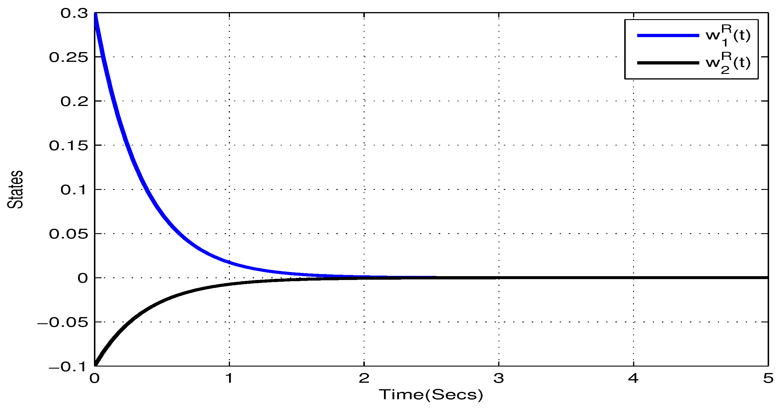
Figure 1. State trajectory of w 1 R ( t ) , w 2 R ( t ) of systems (22) in Example 1.
Mathematics 08 00422 g001
Figure 2. State trajectory of w 1 I ( t ) , w 2 I ( t ) of systems (22) in Example 1.
Mathematics 08 00422 g002
Figure 3. State trajectory of w 1 K ( t ) , w 2 K ( t ) of systems (22) in Example 1.
Mathematics 08 00422 g003
Figure 4. State trajectory of w 1 K ( t ) , w 2 K ( t ) of systems (22) in Example 1.
Mathematics 08 00422 g004
Figure 5. State trajectory of w 1 R ( t ) , w 2 R ( t ) of systems (23) with state feedback control u 1 = 0 , u 2 = 0 in Example 2.
Mathematics 08 00422 g005
Figure 6. State trajectory of w 1 I ( t ) , w 2 I ( t ) of systems (23) with state feedback control u 1 = 0 , u 2 = 0 in Example 2.
Mathematics 08 00422 g006
Figure 7. State trajectory of w 1 J ( t ) , w 2 J ( t ) of systems (23) with state feedback control u 1 = 0 , u 2 = 0 in Example 2.
Mathematics 08 00422 g007
Figure 8. State trajectory of w 1 K ( t ) , w 2 K ( t ) of systems (23) with state feedback control u 1 = 0 , u 2 = 0 in Example 2.
Mathematics 08 00422 g008
Figure 9. State trajectory of w 1 R ( t ) , w 2 R ( t ) of systems (23) with state feedback control u 1 = 0.12 a 1 ( t ) , u 2 = 0.42 a 2 ( t ) in Example 2.
Mathematics 08 00422 g009
Figure 10. State trajectory of w 1 I ( t ) , w 2 I ( t ) of systems (23) with state feedback control u 1 = 0.12 b 1 ( t ) , u 2 = 0.42 b 2 ( t ) in Example 2.
Mathematics 08 00422 g010
Figure 11. State trajectory of w 1 J ( t ) , w 2 J ( t ) of systems (23) with state feedback control u 1 = 0.12 c 1 ( t ) , u 2 = 0.42 c 2 ( t ) in Example 2.
Mathematics 08 00422 g011
Figure 12. State trajectory of w 1 K ( t ) , w 2 K ( t ) of systems (23) with state feedback control u 1 = 0.12 d 1 ( t ) , u 2 = 0.42 d 2 ( t ) in Example 2.
Mathematics 08 00422 g012