Neural-Impulsive Pinning Control for Complex Networks Based on V-Stability

Abstract

In this work, a neural impulsive pinning controller for a twenty-node dynamical discrete complex network is presented. The node dynamics of the network are all different types of discrete versions of chaotic attractors of three dimensions. Using the V-stability method, we propose a criterion for selecting nodes to design pinning control, in which only a small fraction of the nodes is locally controlled in order to stabilize the network states at zero. A discrete recurrent high order neural network (RHONN) trained with extended Kalman filter (EKF) is used to identify the dynamics of controlled nodes and synthesize the control law.

1. Introduction

In recent years, complex networks have been gaining more attention in the scientific community, with a wide range of applications, from computer science to sociology [1]. From the perspective of dynamical systems, it is possible to see a complex network as a group of interconnected systems, each one with their own dynamics and characteristics. For dynamical systems, it is often desirable to force them to follow a desired behavior, which can be performed with a controller. There are many techniques in control theory that have been developed over the years in order to achieve stability around a given equilibrium point [2]. Using a particular method of control depends on the designer or the type of system that is being worked on. A technique developed for the control of complex dynamical networks is pinning control, which consists of controlling only a small fraction of nodes of a complex network [3]. Numerous studies have been published around this pinning control technique, of particular interest to this study is the one of V-stability [4], in which the stability problem for a complex network with different dynamics in its nodes is transformed to verify positive definiteness of an associated matrix.

Another technique not particular to complex networks is impulsive control, which consists of applying a control input in a non-continuous way and is carried out at rather well-defined time instants [5]. The control and synchronization of complex networks through an impulsive input has been studied previously, as in [6], where they propose a control method for a complex network where all node dynamics are the same, similar to [7]. In [8], different node dynamics are proposed, but no pinning control [8].

On the other side, neural networks have long been studied for use in dynamical systems as they have the capacity to reconstruct nonlinear dynamics [9,10] by only having measurements of the system state, which is the case of the neural identifier; then, the output and the model of this neural network can be used to compute a desired control action.

The control and synchronization of complex networks is an active research area. In [11], V-stability and inverse optimal control were used to control a complex network with different chaotic node dynamics. We use this approach in order to interpret the problem of stability of the network as a linear algebra problem that makes it easier to decide the node and gain selection. A discrete-time neural-network was used in [12,13] to synchronize a continuous-time dynamical complex network with an inverse optimal control and sliding mode approach respectively. This work also makes use of neural identification for the great advantage that it represents, accounting for unmodeled behavior and disturbances, which is a matter of study in this work. In [14], a neural network was used to control the network along with V-stability analysis to determine the pinned node. Most of these previous works deal with continuous-time complex networks [12,13,14], but not discrete nor impulsive complex networks. We aim to study discrete-time complex networks for their relevance, as any system governed by a computer processor is essentially discrete. A robotic system network may be a good fit to exemplify this case. For impulsive systems, there are few works that deal with discrete systems. In [15], there is a compilation of distinct stability analysis for impulsive systems like the one in [16], where they show stability conditions for a specific type of discrete-time impulsive systems, which is that the impulse dynamics are linear. This is something that often appears in impulse systems [15]. This is not the case of the study presented here, as will be seen in later sections. Impulsive complex network systems are also important for their potential use in biomedicine. Practical stability for impulsive systems was investigated in [17], where they consider impulsive perturbations and h-manifolds.

The focus of this paper is based on V-stability and an experimental approach, where we work together the different control schemes mentioned above in order to control a discrete-time complex network with different dynamics in its nodes, with an impulsive control law that is synthesized with the neural model. The controller presented in this paper has characteristics of the different control schemes that conform it, like the unnecessariness of the dynamic model, reducing process cost, and reducing the number of local controllers in the complex network.

The remains of this paper is organized as follows. First, complex networks and their dynamical model are briefly described. Then, the concept of V-stability and the process of selecting nodes to control is described. After that, the parameters used in simulations are introduced. Later, impulsive systems are briefly explained, and we present the model used for the impulsive control simulations. Then, recurrent high order neural networks and the identifier used in this paper are discussed. After that, the results are presented and discussed. Lastly, a conclusion of this work is presented.

2. Some Complex Network Theory

Complex networks can be described as a set of $N$ nodes in which any pair of nodes in the set may be connected by a link. This connection between nodes may be directed or undirected and can also be weighted. The number of connections a node has is called the degree and is often denoted by the letter $k$. This letter $k$ is of much importance to complex networks since one can assume several properties based on the distribution of node degrees in the network [18]. Degree distribution in form of a power law, for example, is called a scale-free network, and this kind of network shows a few nodes with a large number of connections and a majority of nodes with a small number of these connections [19].

Nodes of a complex network and their connections can have different meanings [20]. Our interest here is to consider the nodes as dynamical systems and the connection between them as communication between the different node dynamics that together form a bigger and more complex system.

Consider then, the next dynamical model of a complex network with $N$ nodes and linear and diffusive connections [11].

$$\begin{array}{cc}{\dot{x}}_i=f_i\left(x_i\right)+{\displaystyle \sum _{j=1}^N}{c}_{ij}{a}_{ij}\mathsf{\Gamma }{x}_j,& i=1,2,\dots ,N,\end{array}$$

(1)

where $x_i={\left[x_{i1},x_{i2},\dots ,x_{in}\right]}^{\top }$ is the state vector of node $i$. Function $f_i:{ℝ}^n\to {ℝ}^n$ represents the self-dynamics of node $i$. Constant $c_{ij}$ is the connection strength between node $i$ and node $j$. Matrix $A=\left[a_{ij}\right]\in {ℝ}^{N\times N}$ is an outer coupling matrix that describes the network topology, with $a_{ij}=a_{ji}=1$ when there is a connection between node $i$ and node $j$, $a_{ij}=a_{ji}=0$ when there is no connection between node $i$ and node $j$, and when $i=j$, the diagonal elements of matrix $A$ are $a_{ii}=-k_i$, where $k_i$ is the degree (number of connections) of node $i$. The symmetry of matrix $A$ indicates that the connections are undirected. Matrix $\mathsf{\Gamma }\in {ℝ}^{n\times n}$ is an inner coupling matrix that describes the connections between different components of the state vector.

There are previous works about how to drive system (1) to stability [1]. A very common method is the pinning control approach, in which only a few nodes of the network are controlled (or even just one node) [1,3], the nodes selected for control is still a matter of research but in [3] it was found that for scale-free networks, selecting the largest nodes (nodes with the largest number of connections) is most useful.

3. V-Stability

The theoretical analysis presented in this paper is based on the theorem of V-stability presented in [4], under this premise we must find a common Lyapunov function $V\left(x\right)$ for each node dynamics that satisfies:

$$\frac{\partial V\left(x_i\right)}{\partial x_i}\left(f_i\left(x_i\right)-{\theta }_i\mathsf{\Gamma }\left(\overline{x}-x_i\right)\right)<0,$$

(2)

for all $x_i\in D$, where $D$ is equal to the union of all $D_i=\left\{x_i:\Vert x_i-\overline{x}\Vert <\alpha ,\alpha >0\right\}$, $\overline{x}$ is the equilibrium point. As long as this condition holds for the nodes’ self-dynamics, then the V-stability methodology can be applied to any given network [4]. The constant ${\theta }_i$ is called the passivity degree and is not unique, the theoretical passivity degree is defined to be the largest one, but in practice, any value that satisfies the inequality may be chosen [4]. The physical meaning of this method is that there is an energy-like function that is common to all nodes, such that the energy of said function is decreasing along with the evolution of node dynamics. A positive passivity degree means that the node is stable and that it can provide some energy to stabilize the network. A negative passivity degree, on the other hand, means that the node needs energy from the outside to be stable [4]. This method depends greatly on the function $V\left(x\right)$ and constants ${\theta }_i$, that is why it is called V-stability.

If we use a quadratic Lyapunov function of the form $V\left(x\right)=x^{\top }Qx$, where $Q$ is a symmetric and positive definite matrix, then we can change the original stability problem to check if the following inequality is true:

$$C_o=-\mathsf{\Theta }+G\le 0,$$

(3)

where matrix $\mathsf{\Theta }$ is a diagonal matrix with passivity degrees ${\theta }_i$ as its elements, and matrix $G=\left[g_{ij}\right]=\left[c_{ij}{a}_{ij}\right]$. The network (1) is V-stable if (3) is true.

For an unstable network, we can stabilize it with a control action. As mentioned before, with pinning control we can control a network by just controlling a small fraction of the nodes which is more practical than controlling every node of the network. For this purpose, we check the eigenvalues of matrix $C_o$, and if has $m$ non-negative eigenvalues then we need at least $m$ nodes selected for control [4]. The characteristic matrix of a controlled network is:

$$C=-\theta +G-K,$$

(4)

where $K\in {ℝ}^{N\times N}$ is a diagonal matrix with $m$ elements $d_i$ and the remaining elements equal to zero. Elements $d_i$ must be chosen such that characteristic matrix $C$ is negative definite. The values selected can be seen as the feedback gain in the control input $u\left(x\right)$ of the form:

$$u\left(x_i\right)=-d_i{x}_i,$$

(5)

for all the nodes selected for control.

4. Simulation Preliminaries

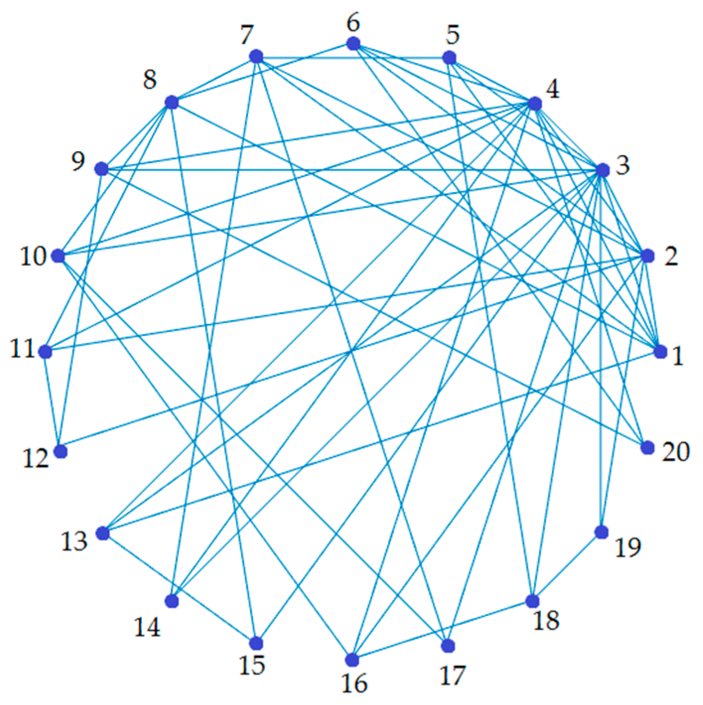
Here, we introduce the 20-node network, with some scale-free characteristics, used for the experiments shown in this paper. This network is illustrated in Figure 1.

For coding purposes, we consider a discrete version of the model (1) with a control input for the nodes selected for control:

$$x_i\left(k+1\right)=x\left(k\right)+T\left(f_i\left(x_i\left(k\right)\right)+{\displaystyle \sum }_{j=1}^N{c}_{ij}{a}_{ij}\mathsf{\Gamma }{x}_j\left(k\right)+u_i\left(x_i\left(k\right)\right)\right),$$

(6)

where $T$ is the sampling time. Parameters of the network are:

$$A=\left[\begin{array}{cc}{A}_1& A_2\\ A_3& A_4\end{array}\right],$$

(7)

where

$$A_1=\left[\begin{array}{cccccccccc}-7& 1& 1& 1& 1& 0& 1& 1& 0& 0\\ 1& -9& 1& 1& 0& 1& 1& 0& 0& 0\\ 1& 1& -13& 1& 1& 1& 0& 0& 1& 1\\ 1& 1& 1& -12& 1& 1& 0& 0& 1& 1\\ 1& 0& 1& 1& -5& 0& 1& 0& 0& 0\\ 0& 1& 1& 1& 0& -5& 0& 1& 0& 0\\ 1& 1& 0& 0& 1& 0& -6& 1& 0& 0\\ 1& 0& 0& 0& 0& 1& 1& -7& 1& 1\\ 0& 0& 1& 1& 0& 0& 0& 1& -5& 0\\ 0& 0& 1& 1& 0& 0& 0& 1& 0& -5\end{array}\right].$$

$$A_2=\left[\begin{array}{cccccccccc}0& 0& 1& 0& 0& 0& 0& 0& 0& 0\\ 1& 1& 0& 0& 0& 1& 0& 0& 1& 0\\ 0& 0& 1& 1& 1& 0& 1& 1& 1& 0\\ 1& 0& 1& 1& 0& 1& 0& 0& 0& 1\\ 0& 0& 0& 0& 0& 0& 0& 1& 0& 0\\ 0& 0& 0& 0& 0& 0& 0& 0& 0& 1\\ 0& 0& 0& 1& 0& 0& 1& 0& 0& 0\\ 1& 0& 0& 0& 1& 0& 0& 0& 0& 0\\ 0& 1& 0& 0& 0& 0& 0& 0& 0& 1\\ 0& 0& 0& 0& 0& 1& 1& 0& 0& 0\end{array}\right].$$

$$A_3=\left[\begin{array}{cccccccccc}0& 1& 0& 1& 0& 0& 0& 1& 0& 0\\ 0& 1& 0& 0& 0& 0& 0& 1& 0& 0\\ 1& 0& 1& 1& 0& 0& 0& 0& 0& 0\\ 0& 0& 1& 1& 0& 0& 1& 0& 0& 0\\ 0& 0& 1& 0& 0& 0& 0& 1& 0& 0\\ 0& 1& 0& 1& 0& 0& 0& 0& 0& 1\\ 0& 0& 1& 0& 0& 0& 1& 0& 0& 1\\ 0& 0& 1& 0& 1& 0& 0& 0& 0& 0\\ 0& 1& 1& 0& 0& 0& 0& 0& 0& 0\\ 0& 0& 0& 1& 0& 1& 0& 0& 1& 0\end{array}\right].$$

$$A_4=\left[\begin{array}{cccccccccc}-4& 1& 0& 0& 0& 0& 0& 0& 0& 0\\ 1& -3& 0& 0& 0& 0& 0& 0& 0& 0\\ 0& 0& -4& 0& 1& 0& 0& 0& 0& 0\\ 0& 0& 0& -3& 0& 0& 0& 0& 0& 0\\ 0& 0& 1& 0& -3& 0& 0& 0& 0& 0\\ 0& 0& 0& 0& 0& -4& 0& 1& 0& 0\\ 0& 0& 0& 0& 0& 0& -3& 0& 0& 0\\ 0& 0& 0& 0& 0& 1& 0& -4& 1& 0\\ 0& 0& 0& 0& 0& 0& 0& 1& -3& 0\\ 0& 0& 0& 0& 0& 0& 0& 0& 0& -3\end{array}\right].$$

Connection strength $c_{ij}$ is equal to all nodes and is chosen as:

$$c_{ij}=c=100.$$

(8)

Matrix $\mathsf{\Gamma }$ is an identity matrix of the order of the state, which is 3:

$$\mathsf{\Gamma }=\left[\begin{array}{ccc}1& 0& 0\\ 0& 1& 0\\ 0& 0& 1\end{array}\right].$$

(9)

Control input is:

$$u_i\left(x_i\left(k\right) \right)=-d_i{x}_i\left(k\right),$$

(10)

with constant $d_i>0$ and only when node $i$ is selected control, if not, the control input is zero. Node self-dynamics are determined by the equations of the following chaotic attractors:

$$\begin{array}{cc}{f}_i\left(x_i\left(k\right)\right)=\left[\begin{array}{c}10\left(x_{i2}\left(k\right)-x_{i1}\left(k\right)\right)\\ 28x_{i1}\left(k\right)-x_{i1}\left(k\right)x_{i3}\left(k\right)-x_{i2}\left(k\right)\\ x_{i1}\left(k\right)x_{i2}\left(k\right)-b{x}_{i3}\left(k\right)\end{array}\right],& i=1,6,11,16,\end{array}$$

(11)

which is the Lorenz system with its parameters as they appear in [21].

$$\begin{array}{cc}{f}_i\left(x_i\left(k\right)\right)=\left[\begin{array}{c}35\left(x_{i2}\left(k\right)-x_{i1}\left(k\right)\right)\\ -7x_{i1}\left(k\right)-x_{i1}\left(k\right)x_{i3}\left(k\right)+28x_{i2}\left(k\right)\\ x_{i1}\left(k\right)x_{i2}\left(k\right)-3x_{i3}\left(k\right)\end{array}\right],& i=2,7,12,17,\end{array}$$

(12)

which is the Chen system with its parameters as they appear in [22].

$$\begin{array}{cc}{f}_i\left(x_i\left(k\right)\right)=\left[\begin{array}{c}36\left(x_{i2}\left(k\right)-x_{i1}\left(k\right)\right)\\ 15x_{i2}\left(k\right)-x_{i1}\left(k\right)x_{i3}\left(k\right)\\ x_{i1}\left(k\right)x_{i2}\left(k\right)-3x_{i3}\left(k\right)\end{array}\right],& i=3,8,13,18,\end{array}$$

(13)

which is the Lü system with its parameters as they appear in [23].

$$\begin{array}{cc}{f}_i\left(x_i\left(k\right)\right)=\left[\begin{array}{c}10\left(x_{i2}\left(k\right)-x_{i1}\left(k\right)\right)+x_{i2}\left(k\right)x_{i3}\left(k\right)\\ 25x_{i1}\left(k\right)-x_{i1}\left(k\right)x_{i3}\left(k\right)-x_{i2}\left(k\right)\\ x_{i1}\left(k\right)x_{i3}\left(k\right)-7x_{i3}\left(k\right)\end{array}\right],& i=4,9,14,19,\end{array}$$

(14)

which is the Qi system with its parameters as they appear in [24].

$$\begin{array}{cc}{f}_i\left(x_i\left(k\right)\right)=\left[\begin{array}{c}9.35\left(x_{i2}\left(k\right)-h\left(x_{i1}\left(k\right)\right)\right)\\ x_{i1}\left(k\right)-x_{i2}\left(k\right)+x_{i3}\left(k\right)\\ -14.79x_{i3}\left(k\right)\end{array}\right],& i=5,10,15,20,\end{array}$$

(15)

which is the Chua system with its parameters and:

$$h\left(x_{i1}\left(k\right)\right)=\frac{2}{7}{x}_{i1}\left(k\right)-\frac{3}{14}\left(\left|x_{i1}\left(k\right)+1\right|-\left|x_{i1}\left(k\right)-1\right|\right),$$

(16)

as they appear in [25].

We first make the continuous analysis of V-stability and then we apply the results of this analysis to the discrete network (6). First, we obtain the passivity degree ${\theta }_i$ for each node using the function $V\left(x_i\right)=0.5x_i^{\top }{x}_i$, the equilibrium point $\overline{x}=0$, and inequality (2) obtaining.

$${\theta }_i<\frac{-38x_{i1}{x}_{i2}+10x_{i1}^2+x_{i1}^2+\frac{8}{3}{x}_{i3}^2}{x_{i1}^2+x_{i2}^2+x_{i3}^2},$$

(17)

for the Lorenz system,

$${\theta }_i<\frac{28x_{i1}{x}_{i2}+35x_{i1}^2-28x_{i1}^2+3x_{i3}^2}{x_{i1}^2+x_{i2}^2+x_{i3}^2},$$

(18)

for the Chen system,

$${\theta }_i<\frac{-36x_{i1}{x}_{i2}+36x_{i1}^2-15x_{i1}^2+3x_{i3}^2}{x_{i1}^2+x_{i2}^2+x_{i3}^2},$$

(19)

for the Lü system,

$${\theta }_i<\frac{-38x_{i1}{x}_{i2}+10x_{i1}^2-x_{i1}{x}_{i2}{x}_{i3}+x_{i1}^2+7x_{i3}^2}{x_{i1}^2+x_{i2}^2+x_{i3}^2},$$

(20)

for the Qi system, and

$${\theta }_i<\frac{-10.35x_{i1}{x}_{i2}+9.35h\left(x_{i1}\right)+x_{i1}^2-x_{i2}{x}_{i3}+14-79x_{i3}^2}{x_{i1}^2+x_{i2}^2+x_{i3}^2},$$

(21)

for the Chua system.

It can be seen that there is no clear value for the passivity degrees, it all depends on the set $D$ of interest. Defining an arbitrary set, we obtain the next rough set of values for the passivity degrees shown in

Table 1. Passivity degree values for the different chaotic systems.

Chaotic System	$\mathbf{Passivity}\mathbf{Degree}{\mathit{\theta }}_{\mathit{i}}$
Lorenz	−13.6
Chen	−28.1
Lü	−15.1
Qi	−22.4
Chua	−5.1

.

With these values, we can now construct the diagonal matrix $\mathsf{\Theta }$ and with this, also matrix $C_o$ and we can obtain its eigenvalues. Only one of the eigenvalues results non-negative, meaning that we need at least one controlled node. We thus construct matrix $K$ with only one non-zero element, we select the element $d_3$ to be non-zero so we control node 3, based on the number of its connections. If we select $d_3=500$ and check for the eigenvalues of $C$, we can verify that the matrix is now negative definite which means that the network is now stable. A MATLAB^® simulation of the resulting dynamics using sample time $T=0.001$ can be seen in Figure 2.

The concept of V-stability refers to a characterization of node stability. The passivity degree expresses how stable or unstable the node in question is. In case the system is stable, we could verify the gain in which the system becomes unstable (in case of such gain exists). In the unstable case, we search for the gain in which the system becomes stable, like we did in this section. The advantage of this characterization is that it defines the stability of a given network with the negativity of matrix (3) (or (4) when it is in a closed loop), this facilitates the node selection by establishing the number of non-negative eigenvalues which is the minimum number of pinned nodes to control.

5. Impulsive Systems

Our goal is not to verify the V-stability method, which gives an interesting result on how many nodes to control, but to apply it while using a neural network as an identifier in order to synthesize control law for the controlled node state, and also verify how it works under and impulsive control scheme and noise conditions.

A time-dependent impulsive system in simple form can be written as [5]:

$$\begin{array}{cc}\dot{x}\left(t\right)=f_c\left(x\left(t\right)\right),& t\ne t_k,\\ \mathsf{\Delta }x\left(t\right)=f_d\left(x\left(t\right)\right),& t=t_k.\end{array}$$

(22)

This means that there is a certain dynamic in the system given by $f_c(\cdot )$, but when time gets to $t_k$, it changes to $f_d(\cdot )$ just for that time instant.

Extrapolating this to our complex network discrete model (6), we can write our system as:

$$\begin{array}{cc}{x}_i\left(k+1\right)=x\left(k\right)+T\left(f_i\left(x_i\left(k\right)\right)+{\displaystyle \sum _{j=1}^N}{c}_{ij}{a}_{ij}\mathsf{\Gamma }{x}_j\left(k\right)\right)& Tk\ne t_k\\ x_i\left(k+1\right)=x\left(k\right)+T\left(f_i\left(x_i\left(k\right)\right)+{\displaystyle \sum _{j=1}^N}{c}_{ij}{a}_{ij}\mathsf{\Gamma }{x}_j\left(k\right)+u_i\left(x_i\left(k\right)\right)\right)& Tk=t_k\end{array}$$

(23)

and $u_i=0$ if node $i$ was not selected for control.

We see that the only thing that changes in the pulse dynamics (when $t=t_k$) is that there is a control input that only appears at time $t_k$. We define $t_k$ as being every $5T$ and every $10T$, this means that control input appears every five times the sample time and every ten times the sample time, whit sample time $T=0.001$, for all simulations.

We cannot be sure the V-stability method works with something like this—that is where the experimentation enters in. Before that, we shall introduce the last concept.

6. Neural Identifier

Artificial neural networks have different applications depending on their configuration [26]. A recurrent high order neural network (RHONN) is good at approximating the behavior of continuous and discrete dynamical systems [9,10].

For a discrete RHONN, we consider the model [10]:

$$\begin{array}{cc}{x}_i\left(k+1\right)=w_i^{\top }{z}_i\left(x\left(k\right),u\left(k\right)\right),& i=1,2,\dots ,n\end{array},$$

(24)

where $x_i\left(k\right)$ is the state of the $i$th neuron at time step $k$, $n$ is the dimensión of the state, $w_i$ is the adaptable weight vector, and $z\left(x\left(k\right),u\left(k\right)\right)$ is defined as:

$$z_I\left(x,u\right)=\left[\begin{array}{c}{z}_{I1}\\ z_{I2}\\ ⋮\\ z_{IL}\end{array}\right]=\left[\begin{array}{c}{\displaystyle \prod }_{j\in I_1}{y}_j^{d_j\left(1\right)}\\ {\displaystyle \prod }_{j\in I_2}{y}_j^{d_j\left(2\right)}\\ ⋮\\ {\displaystyle \prod }_{j\in I_1}{y}_j^{d_j\left(L\right)}\end{array}\right],$$

(25)

where $L$ is the number of high order connections, $\left\{I_1,I_2,\dots ,I_L\right\}$ is a collection of $L$ unordered subsets $\left\{1,2,\dots ,m+n\right\}$, and $y$ is a vector formed by the inputs of each neuron defined as:

$$y=\left[\begin{array}{c}{y}_1\\ ⋮\\ y_n\\ y_{n+1}\\ ⋮\\ y_{n+m}\end{array}\right]=\left[\begin{array}{c}S\left(x_1\right)\\ ⋮\\ S\left(x_n\right)\\ u_1\\ ⋮\\ u_m\end{array}\right],$$

(26)

vector $u={\left[u_1,u_2,\dots , u_m\right]}^{\top }$ here is the input vector to the neural network. $S(\cdot )$ is a smooth, monotonically increasing sigmoid function [10,21].

The discrete RHONN can be trained by using the extended Kalman filter (EKF) algorithm. Necessary equations for the EKF algorithm are [10,27]:

$$K\left(k\right)=P\left(k\right)H^{\top }\left(k\right){\left[R\left(k\right)+H\left(k\right)P\left(k\right)H^{\top }\left(k\right)\right]}^{-1},$$

(27)

$$w\left(k+1\right)=w\left(k\right)+K\left(k\right)\left[y\left(k\right)-\widehat{y}\left(k\right)\right],$$

(28)

$$P\left(k+1\right)=P\left(k\right)-K\left(k\right)H\left(k\right)P\left(k\right)+Q\left(k\right),$$

(29)

where $K\left(k\right)\in {ℝ}^{m\times L}$ is the Kalman gain matrix. $P\left(k\right)\in {ℝ}^{L\times L}$ represents the error covariance matrix. $H\left(k\right)\in {ℝ}^{m\times L}$ is the matrix containing the derivatives of each network output with respect to each one of the weights, that is:

$$\begin{array}{ccc}{H}_{ij}\left(k\right)=\left[\frac{\partial {\widehat{y}}_i\left(k\right) }{\partial w_j\left(k\right)}\right],& i=1,\dots ,m,& j=1,\dots ,L,\end{array}$$

(30)

$R\left(k\right)\in {ℝ}^{m\times m}$ is the measurement error covariance matrix. $w\in {ℝ}^L$ is the weight vector, $L$ is the number of weights of the neural network. $y\in {ℝ}^m$ is the output vector; $m$ is the number of outputs, $\widehat{y}\in {ℝ}^m$ is the neural network output, the difference of these two represents the error signal. $Q\left(k\right)\in {ℝ}^{L\times L}$ is the process error covariance matrix.

The neural identifier used is based on the described model (24) of discrete RHONN and it has the following structure:

$$\begin{array}{c}{\hat{x}}_{i1}\left(k+1\right)=w_{i11}\left(k\right)\phi \left(x_{i2}\left(k\right)\right)+w_{i21}\left(k\right)\phi \left(x_{i1}\left(k\right)\right)+w_{i31}\left(k\right)\phi \left(x_{i2}\left(k\right)\right)\phi \left(x_{i3}\left(k\right)\right),\\ {\hat{x}}_{i2}\left(k+1\right)=w_{i12}\left(k\right)\phi \left(x_{i1}\left(k\right)\right)+w_{i22}\left(k\right)\phi \left(x_{i1}\left(k\right)\right)\phi \left(x_{i3}\left(k\right)\right)+w_{i32}\left(k\right)\phi \left(x_{i2}\left(k\right)\right),\\ {\hat{x}}_{i3}\left(k+1\right)=w_{i13}\left(k\right)\phi \left(x_{i1}\left(k\right)\right)\phi \left(x_{i2}\left(k\right)\right)+w_{i23}\left(k\right)\phi \left(x_{i3}\left(k\right)\right)+w_{i33}\left(k\right)\phi \left(x_{i2}\left(k\right)\right),\end{array}$$

(31)

where $\phi (\cdot )$ is the sigmoid function:

$$\phi \left(x\right)=0.1\tanh \left(0.05x\right).$$

(32)

The neural network weights $w_{ijl}\left(k\right)$, are obtained by training the RHONN with the EKF algorithm. In this case, subscript $j$ denotes the weight vector element, subscript $l$ denotes the state element to identify, and subscript $i$ is the aimed node identify. Weights are computed separately for each state element. Algorithm equations used for training are the ones in (27), (28) and (29), that become:

$$K_i\left(k\right)=P_i\left(k\right)H_{ij}^{\top }\left(k\right){\left[R_i\left(k\right)+H_{ij}\left(k\right)P_i\left(k\right)H_{ij}^{\top }\left(k\right)\right]}^{-1},$$

(33)

$$w_i\left(k+1 \right)=w_i\left(k\right)+K_i\left(k\right)\left[x_i\left(k\right)-{\widehat{x}}_i\left(k\right)\right],$$

(34)

$$P_i\left(k+1\right)=P_i\left(k\right)-K_i\left(k\right)H_{ij}\left(k\right)P_i\left(k\right)+Q_{ij}\left(k\right),$$

(35)

with initial $P\left(k\right)$:

$$P_i\left(0\right)=\left[\begin{array}{ccc}10& 0& 0\\ 0& 10& 0\\ 0& 0& 10\end{array}\right],$$

(36)

and the rest of the parameters as:

$$\begin{array}{ccc}{H}_{i1}^{\top }=\left[\begin{array}{c}\phi \left(x_{i2}\left(k\right)\right)\\ \phi \left(x_{i1}\left(k\right)\right)\\ \phi \left(x_{i2}\left(k\right)\right)\phi \left(x_{i3}\left(k\right)\right)\end{array}\right],& H_{i1}^{\top }=\left[\begin{array}{c}\phi \left(x_{i2}\left(k\right)\right)\\ \phi \left(x_{i1}\left(k\right)\right)\\ \phi \left(x_{i2}\left(k\right)\right)\phi \left(x_{i3}\left(k\right)\right)\end{array}\right],& H_{i1}^{\top }=\left[\begin{array}{c}\phi \left(x_{i2}\left(k\right)\right)\\ \phi \left(x_{i1}\left(k\right)\right)\\ \phi \left(x_{i2}\left(k\right)\right)\phi \left(x_{i3}\left(k\right)\right)\end{array}\right],\end{array}$$

(37)

$$R_i\left(k\right)=R_i=10,$$

(38)

$$Q_{i1}\left(k\right)=Q_{i2}\left(k\right)=Q_{i3}=Q=\left[\begin{array}{ccc}0.1& 0& 0\\ 0& 0.1& 0\\ 0& 0& 0.1\end{array}\right].$$

(39)

All these parameters were heuristically determined. Initial weight values are positive random values no bigger than 1.

With this, we can synthesize control law as:

$$u_i=-d_i{\widehat{x}}_i$$

(40)

where $d_i$ is estimated by the analysis completed in Section 3 and ${\widehat{x}}_i$ is determined by the network (31).

7. Results

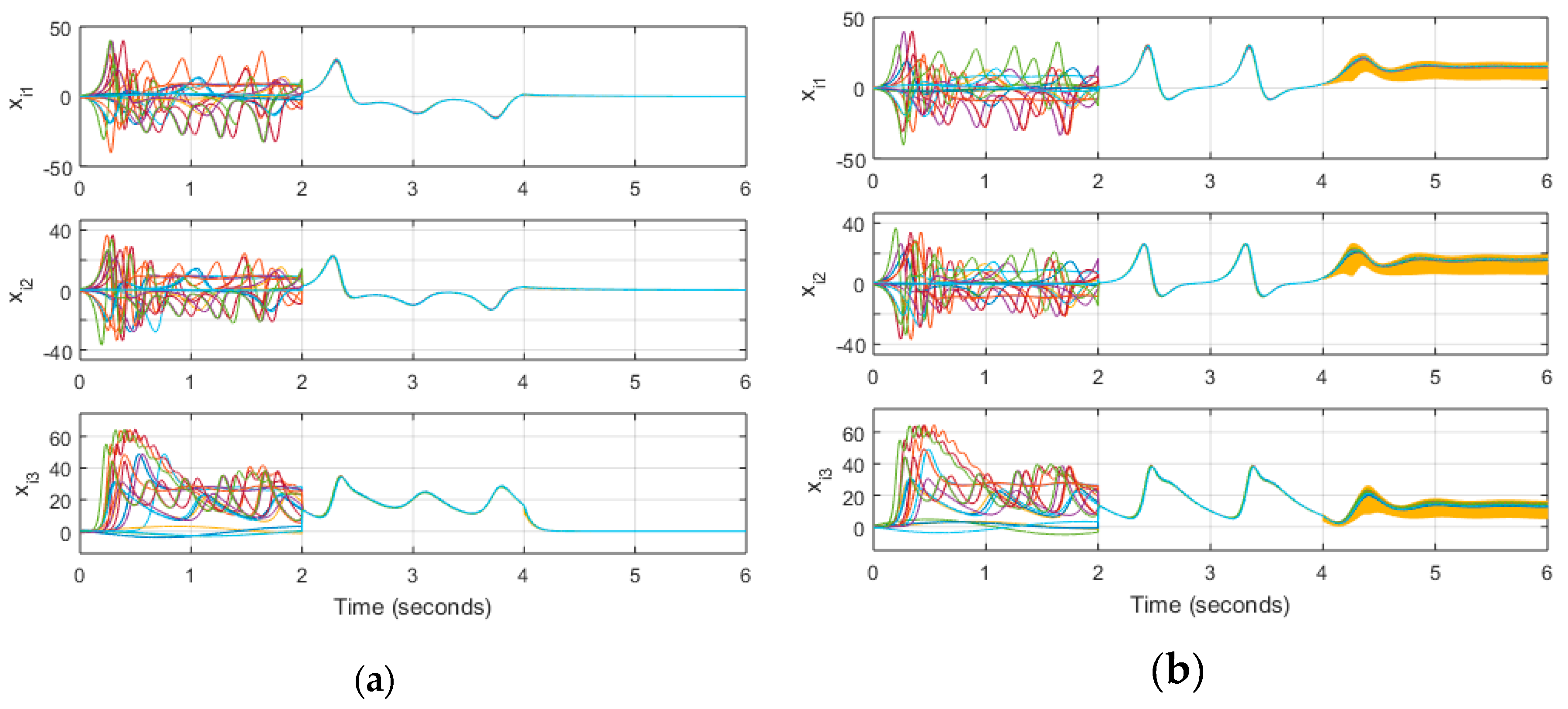
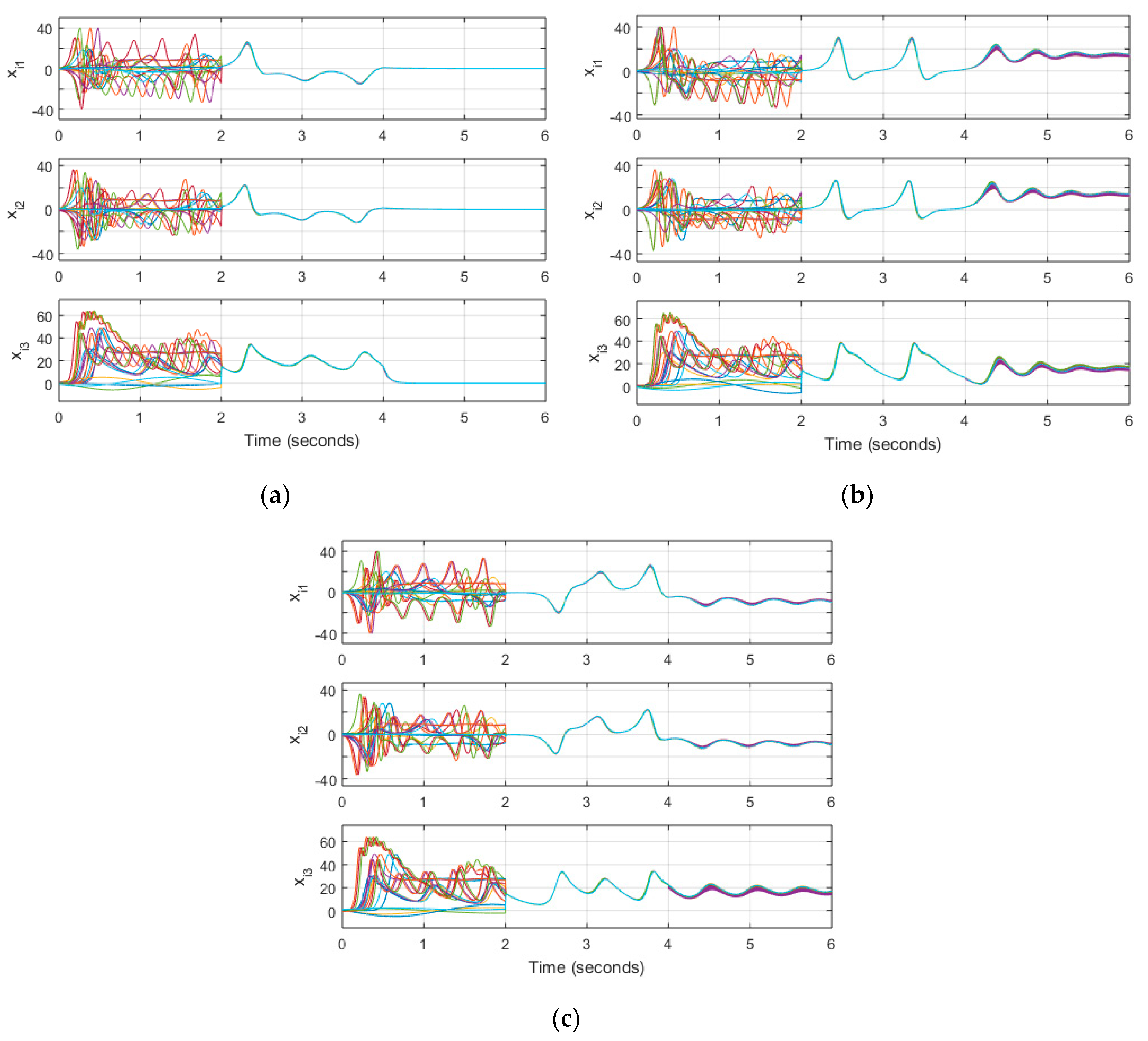
Using the models (6) and (23), with parameters used in Section 4, and neural network parameters mentioned in Section 6, simulations were made in MATLAB^®. One of the experiments is made with the model (6) as it is, and in the other, random noise is added to the system. We make the simulations for three different control schemes:

(a)

Continuous in discrete time

(b)

Control impulses every 5T

(c)

Control impulses every 10T

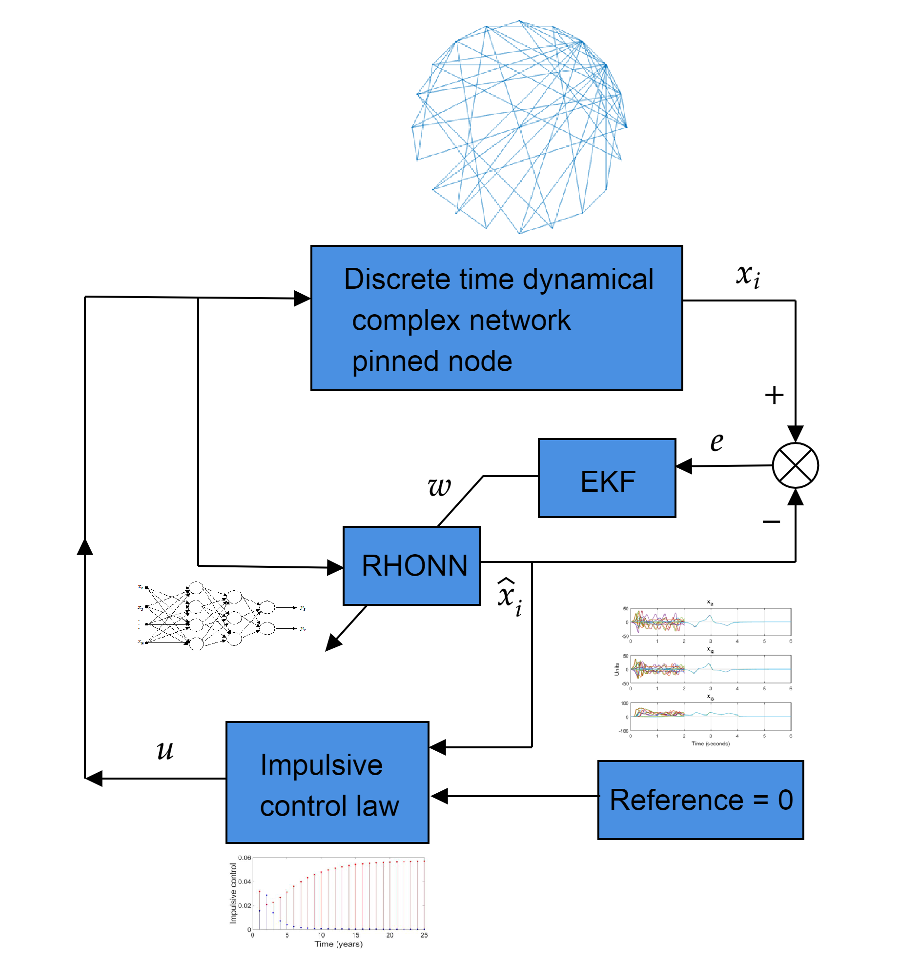
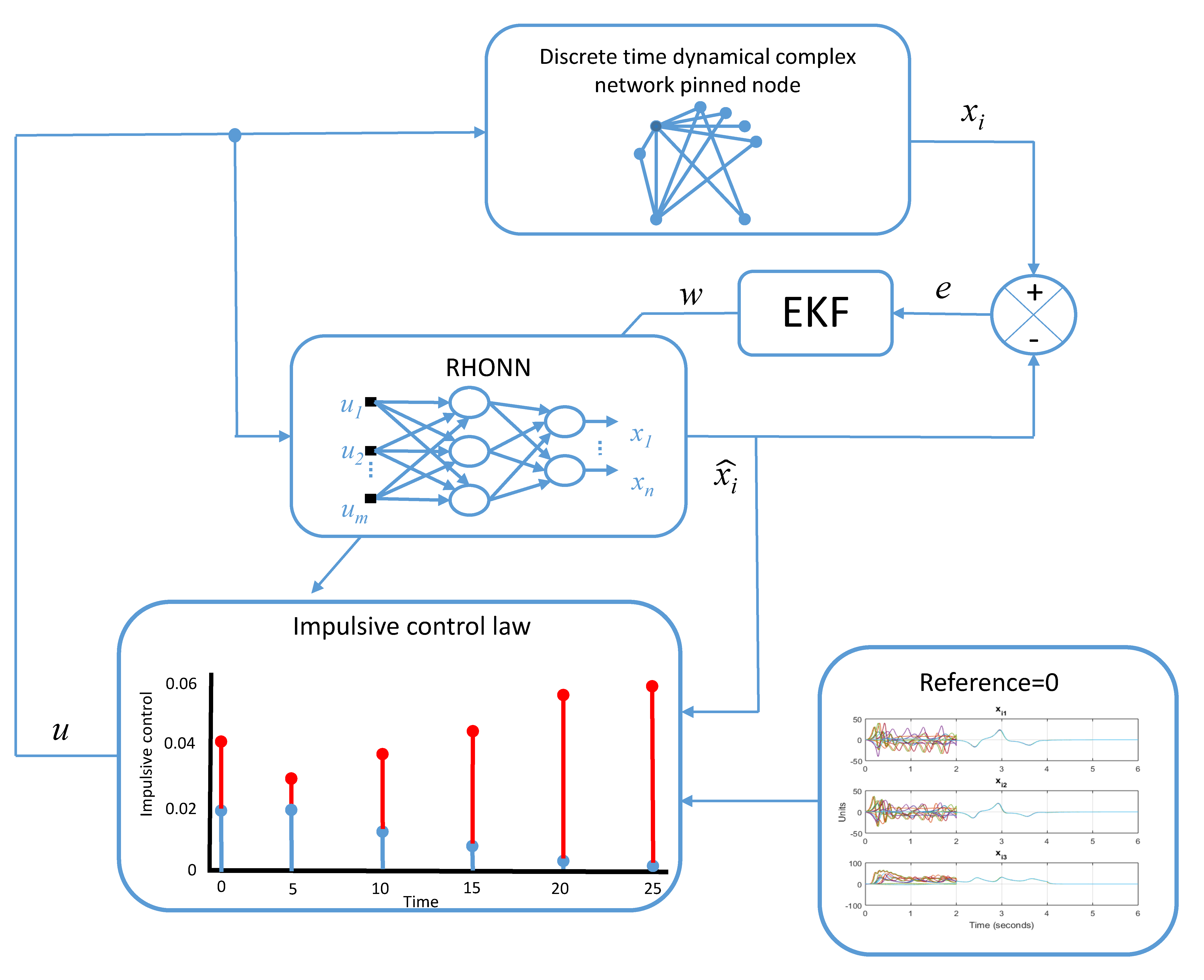
Experiments were carried out as follows. All the nodes are unconnected at the beginning of the simulation. At time 2, the nodes connect with each other according to matrix $A$, matrix $\mathsf{\Gamma }$, and constant $c$, defined in (7), (9), and (8) respectively. At time 4, the synthetized control law appears according to what is observed in (a), (b), and (c). All initial conditions for the node states are random. A general scheme, of the proposed control strategy, is shown in Figure 3.

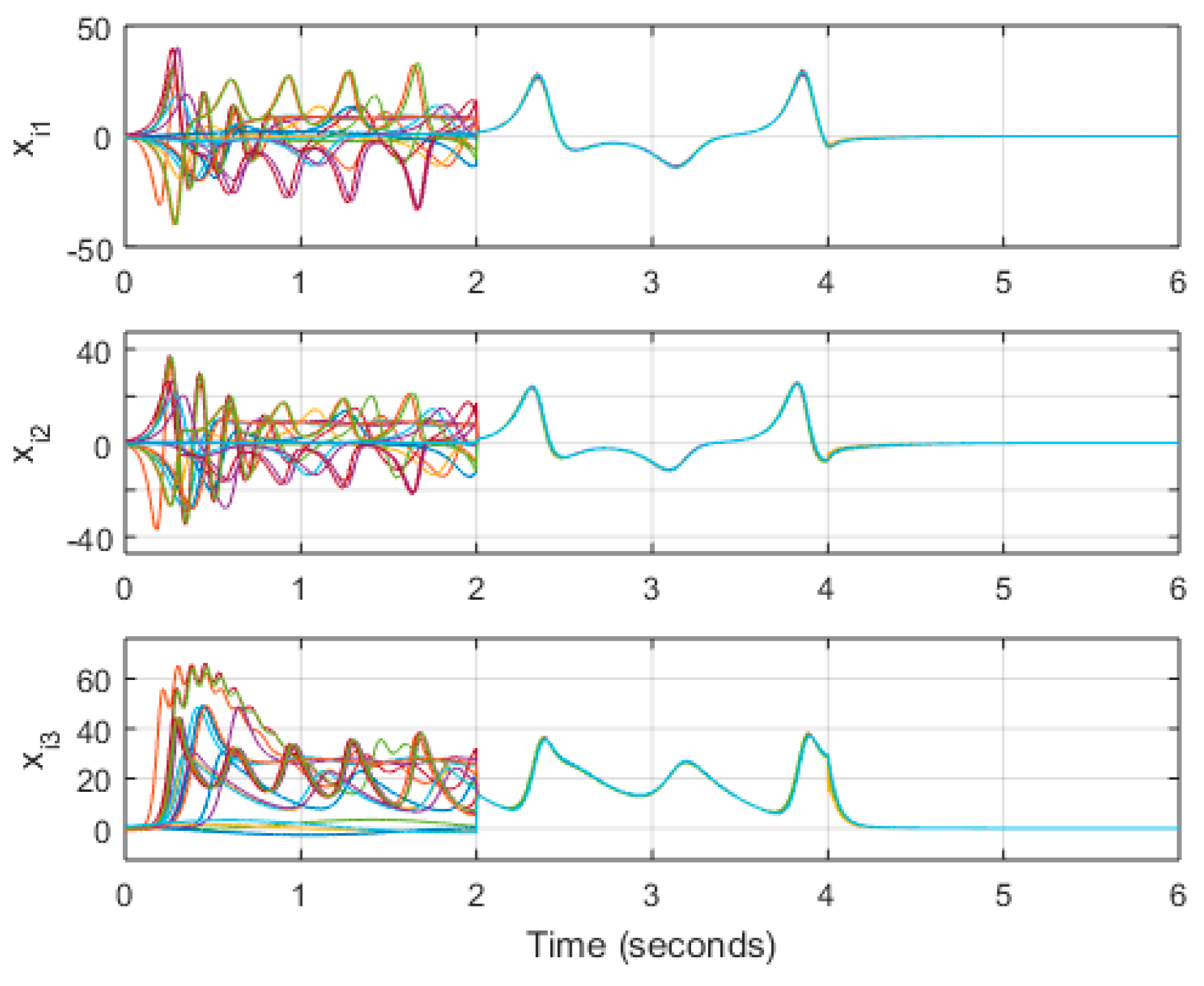
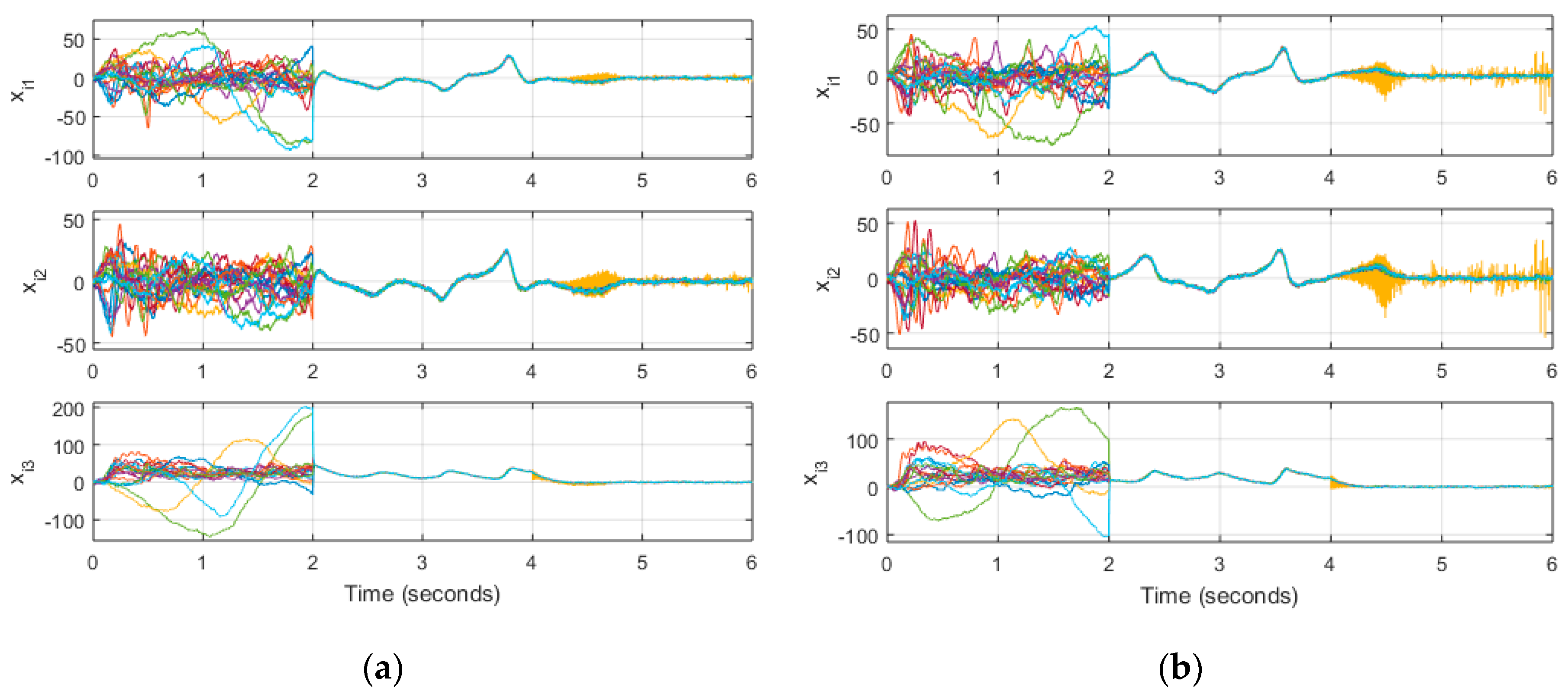
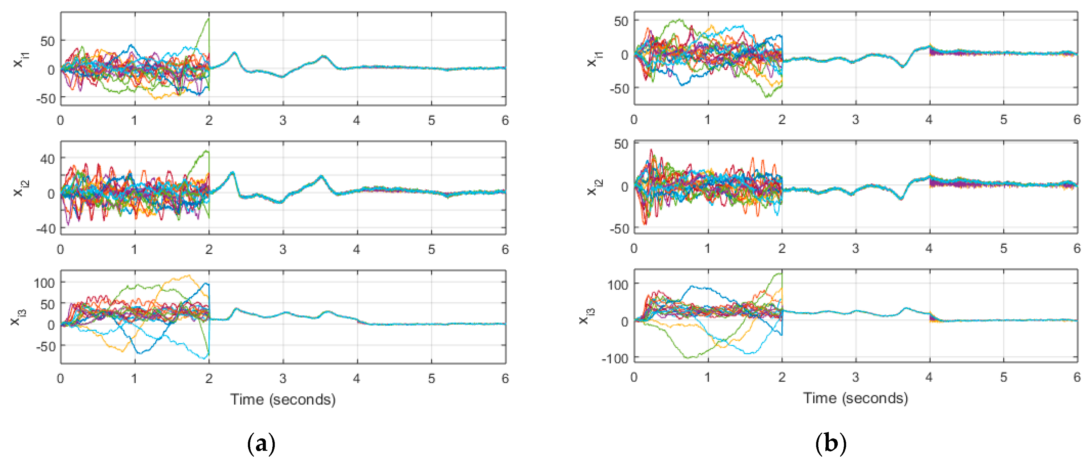
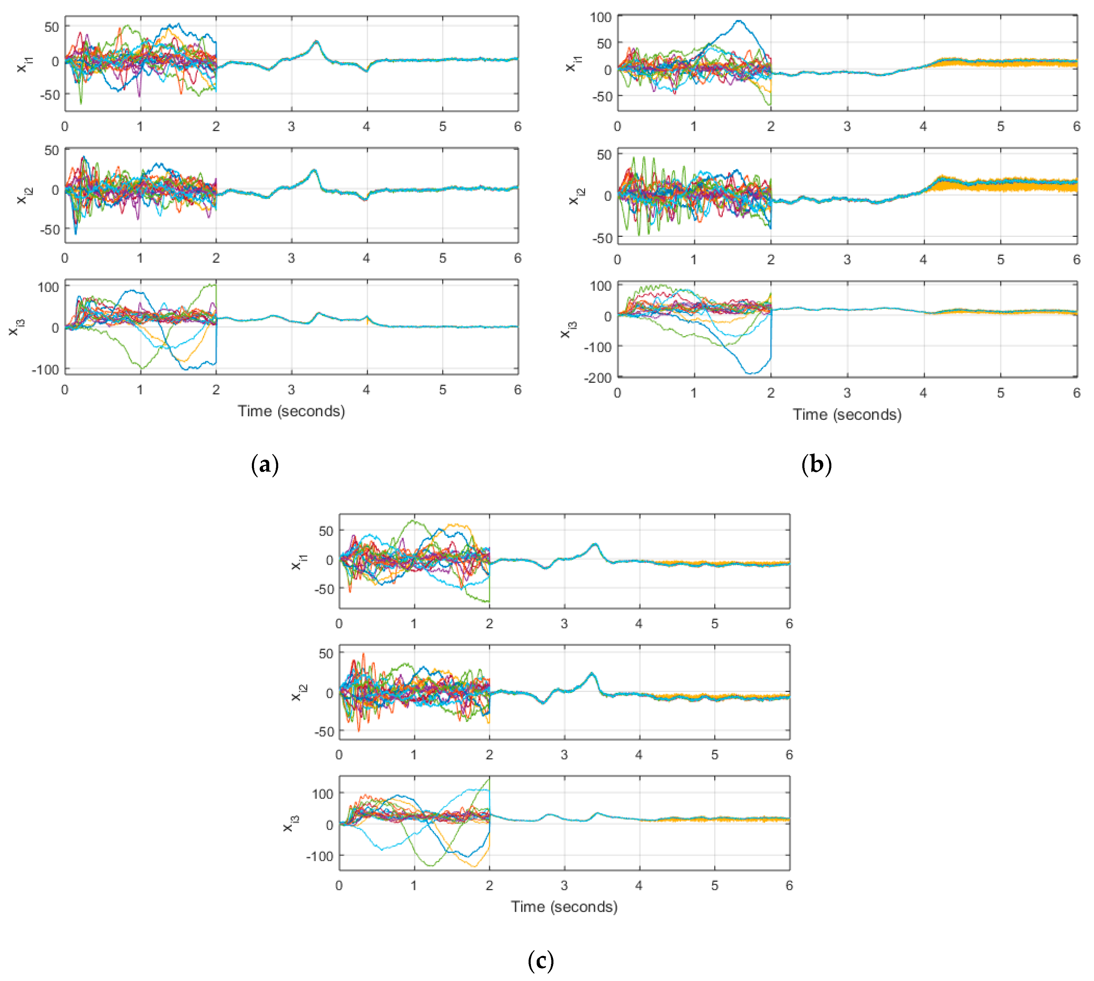
The results of simulations are shown as follows: Figure 4 shows the network dynamics when the system does not have noise for all three control schemes. Figure 5 shows the network dynamics when there is noise in all of the nodes in the network. It is important to note that all of the node self-dynamics are a set of dimensionless chaotic systems.

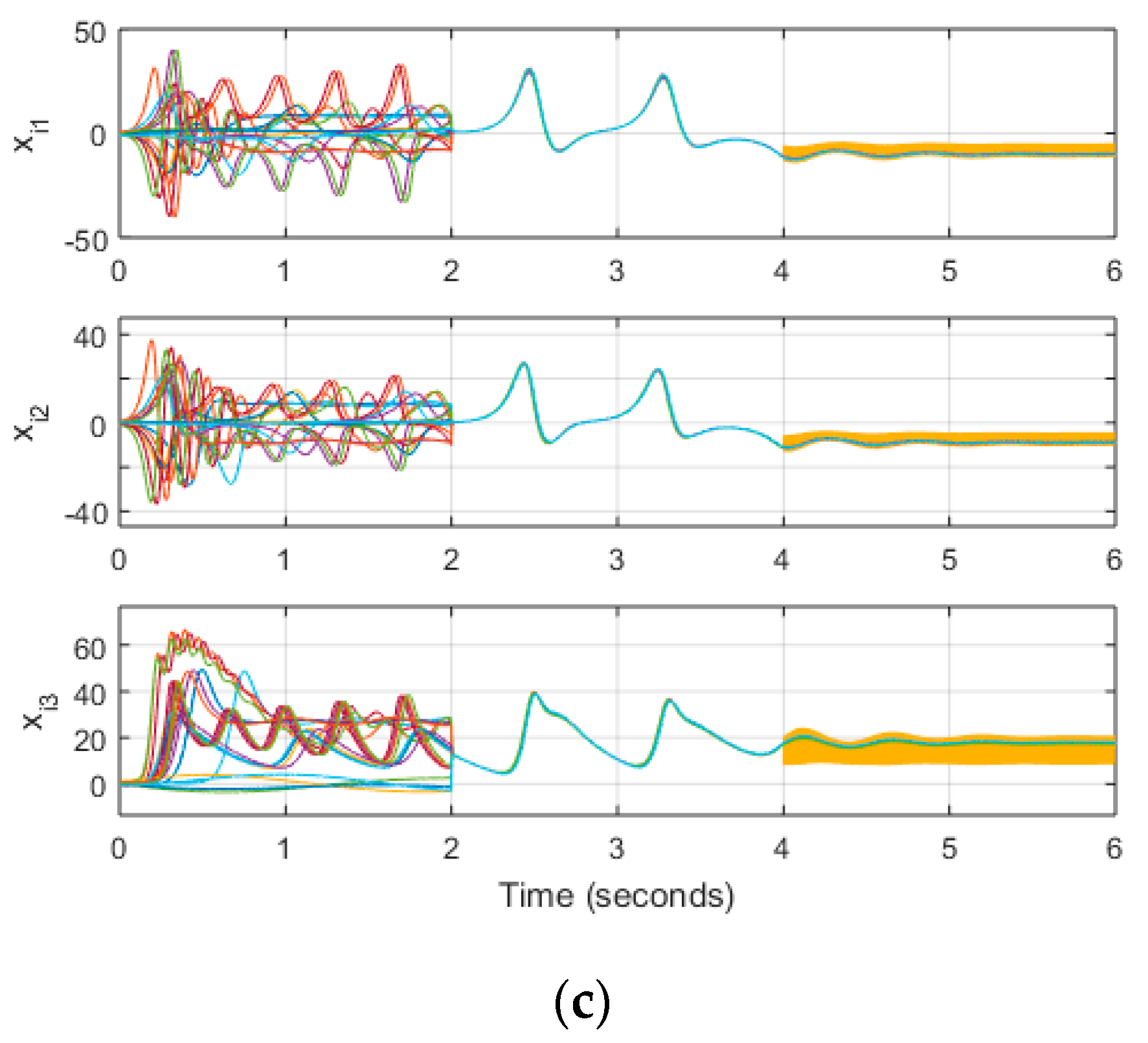
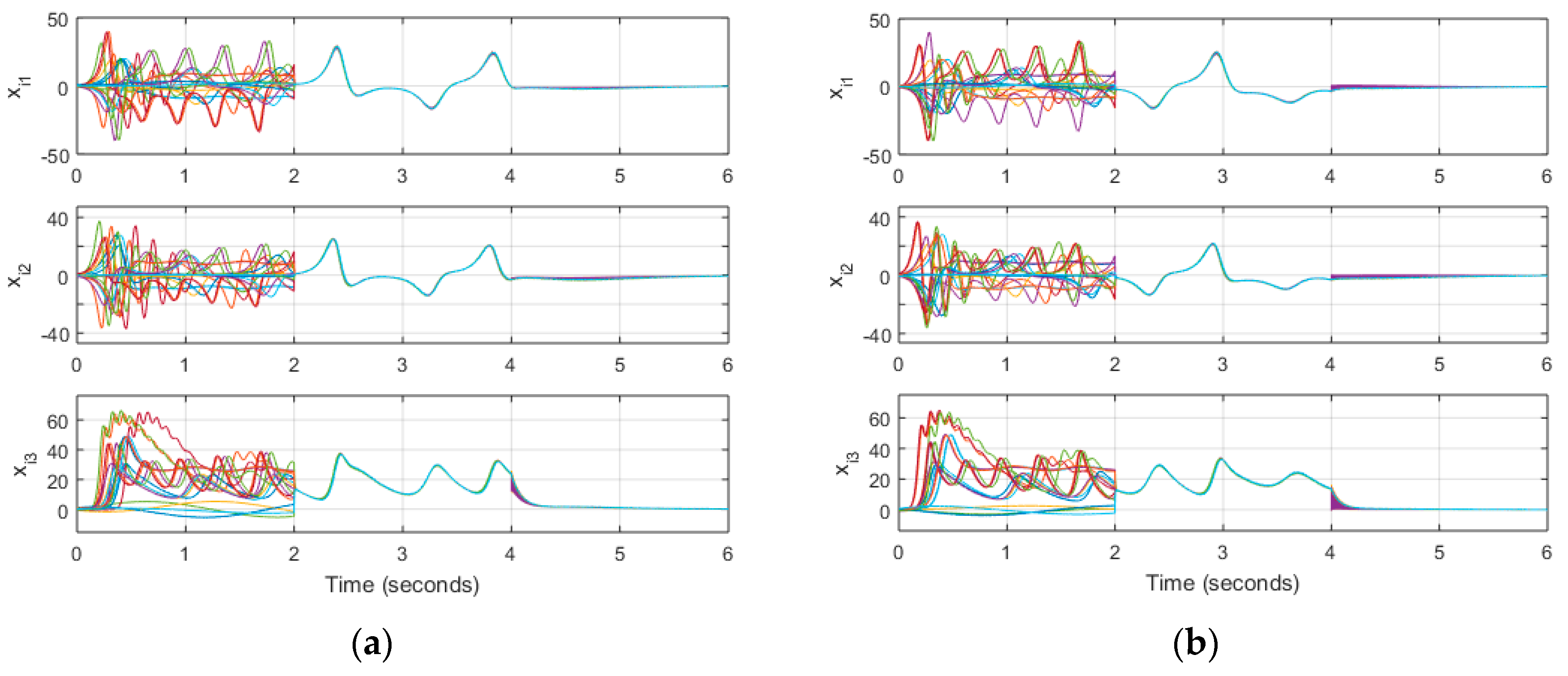
We can observe that the impulsively controlled systems stabilize, but not as close to zero as the one controlled continuously. If we increase the control gain to $d_3=1000$ when the control input is applied every 5T and $d_3=1500$ when the control input is applied every 10T we can obtain better results for the case when there is no noise as shown in Figure 6. Doing the same in for the case with noise, we observe in Figure 7 that we can cause more noise in the system.

8. Discussion

As detailed in Section 5, we could not assure that the V-stability method works for the impulsive control schemes, but completing the analysis provides us with a good idea to how many and what nodes to pin, and we also obtain an estimate for the control gain value.

While we achieve stability in zero with the impulsively controlled unnoisy systems, we had to increase the gain to do it. In the case of noise, we observed more noise; therefore, perhaps another solution is more suitable.

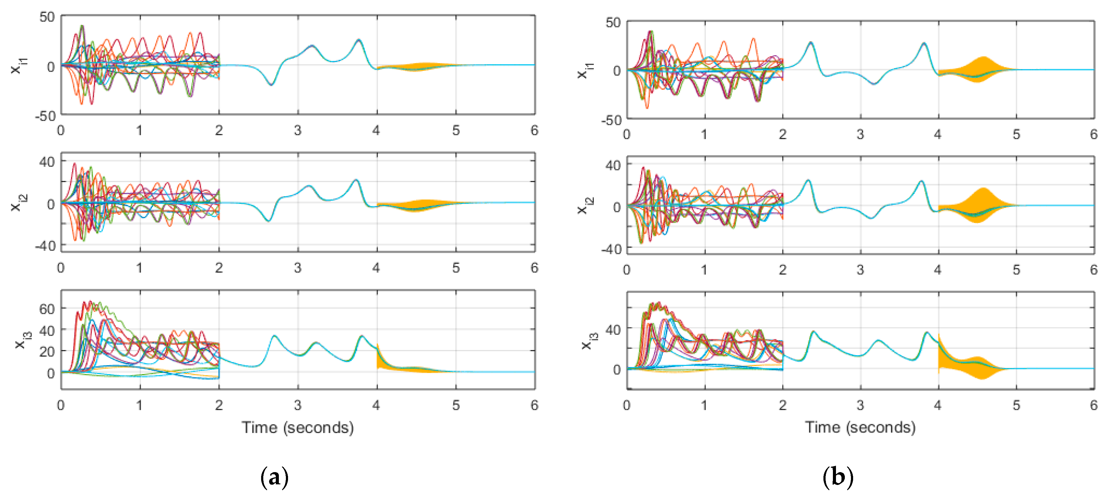
In this kind of problem, it is always very tempting to stabilize the network using only one controller for one node. If we go back to the V-stability concept of Section 3, we can control the network described by matrix (7) with at least one pinned node, and we did this by checking the stability of matrix $C$ in (4) with a matrix $K$ that we designed. We can choose to pin two nodes of the network by making two diagonal elements $d_i$ of $K$ different to zero. Hypothetically, if we make $d_3=d_4=200$, that is, we control nodes 3 and 4, we can verify that by doing this, all eigenvalues of $C$ are negative, which means that the complex network is stable. Running another simulation of the unnoisy and noisy systems for the different schemes provides us with the results of Figure 8 and Figure 9 respectively.

We see that the impulsively controlled network performs similar to its one-pinned node counterpart, but with less than half the energy for both nodes. Increasing the gains to $d_3=d_4=700$ for the 5T case and $d_3=d_4=1200$ for the 10T case, we obtain better results that are shown in Figure 10 for the no-noise case and Figure 11 for the case with noise.

Since a large enough gain can provide adequate performance, it can require inputs with a large amount of energy that are not possible to implement, in such case an option is to select more nodes to pin (but not all of the available nodes).

A formal analysis of the V-stability method for discrete and impulsive complex network systems may be a good direction for future work.

The results show that neural network works and adapts well as the same structure was used to identify the dynamics of node 4 and synthesize its control law.

We can reproduce these results with other networks using different parameters (number of nodes, connections, connection strength, etc.) as long as the self-dynamics of the nodes satisfy condition (2) discussed in Section 3, for some passivity degree $\theta$. It is important to note if that we use the same network as before, but with a connection strength reduced to $c=50$, constructing matrix $C_o$ again and checking for its eigenvalues, we still obtain the information that there is only one non-negative eigenvalue, but setting the same gain $d_3=500$ is not sufficient to make matrix $C$ negative definite. 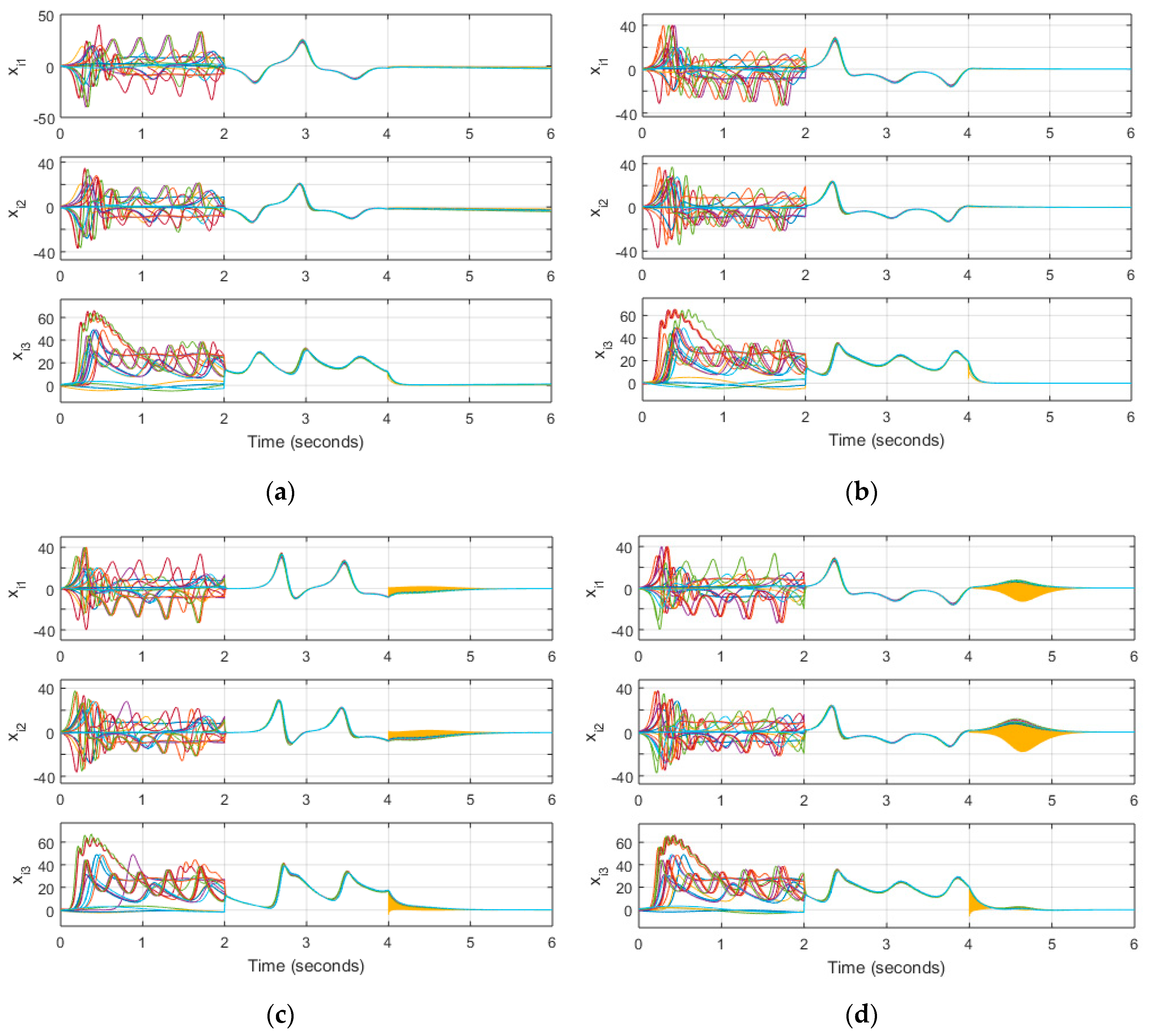Figure 12a shows the network node dynamics with a controller with this gain, and we can see that it starts to diverge from zero at the end of the simulation. If we make $d_3=800$ matrix $C$ will become negative definite, so we use this gain to control the network with a continuous input in discrete time as we see in Figure 12b. Based on the results of Figure 6 and Figure 10, we increase the gain to $d_3=1300$ for the case where the control impulses are every 5T, and $d_3=1800$ for the case where control impulses are every 10T. These last results are shown in Figure 12c,d respectively. These results were also obtained using the RHONN of past simulations.

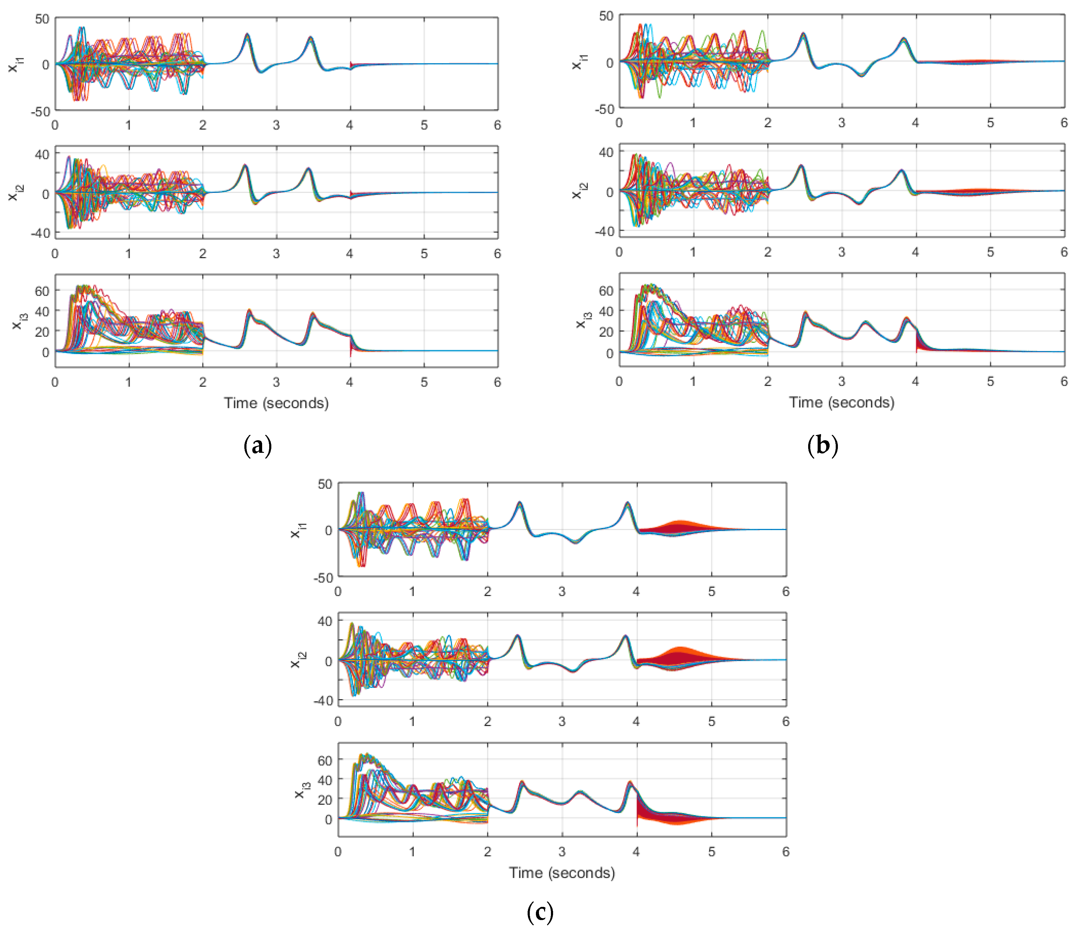
Using a smaller connection strength results in requiring more effort in order to stabilize the network. In fact, if we use a connection strength of $c=1$, the analysis tells us that the minimum number of controllers must be 18. If we use the ten-node network described by matrix (41) with node self-dynamics in the same order as past simulations and a connection strength of $c=100$, from V-stability analysis on this network, we see that the associated matrix $C_o$ has one non-negative eigenvalue, by pinning the first node, that has seven connections to other nodes, with a gain of $d_1=400$ we can make matrix $C$ negative definite. As before, we increase this gain to $d_1=900$ for the case where the control input is applied every 5T and $d_1=1400$ when the control input is applied every 10T, these results can be seen in Figure 13. The RHONN used before was also used here.

$$A=\left[\begin{array}{cccccccccc}-7& 1& 1& 1& 0& 1& 0& 1& 1& 1\\ 1& -5& 1& 1& 1& 0& 1& 0& 0& 0\\ 1& 1& -4& 0& 1& 0& 0& 0& 1& 0\\ 1& 1& 0& -3& 0& 1& 0& 0& 0& 0\\ 0& 1& 1& 0& -3& 0& 0& 1& 0& 0\\ 1& 0& 0& 1& 0& -3& 1& 0& 0& 0\\ 0& 1& 0& 0& 0& 1& -2& 0& 0& 0\\ 1& 0& 0& 0& 1& 0& 0& -3& 0& 1\\ 1& 0& 1& 0& 0& 0& 0& 0& -2& 0\\ 1& 0& 0& 0& 0& 0& 0& 1& 0& -2\end{array}\right].$$

(41)

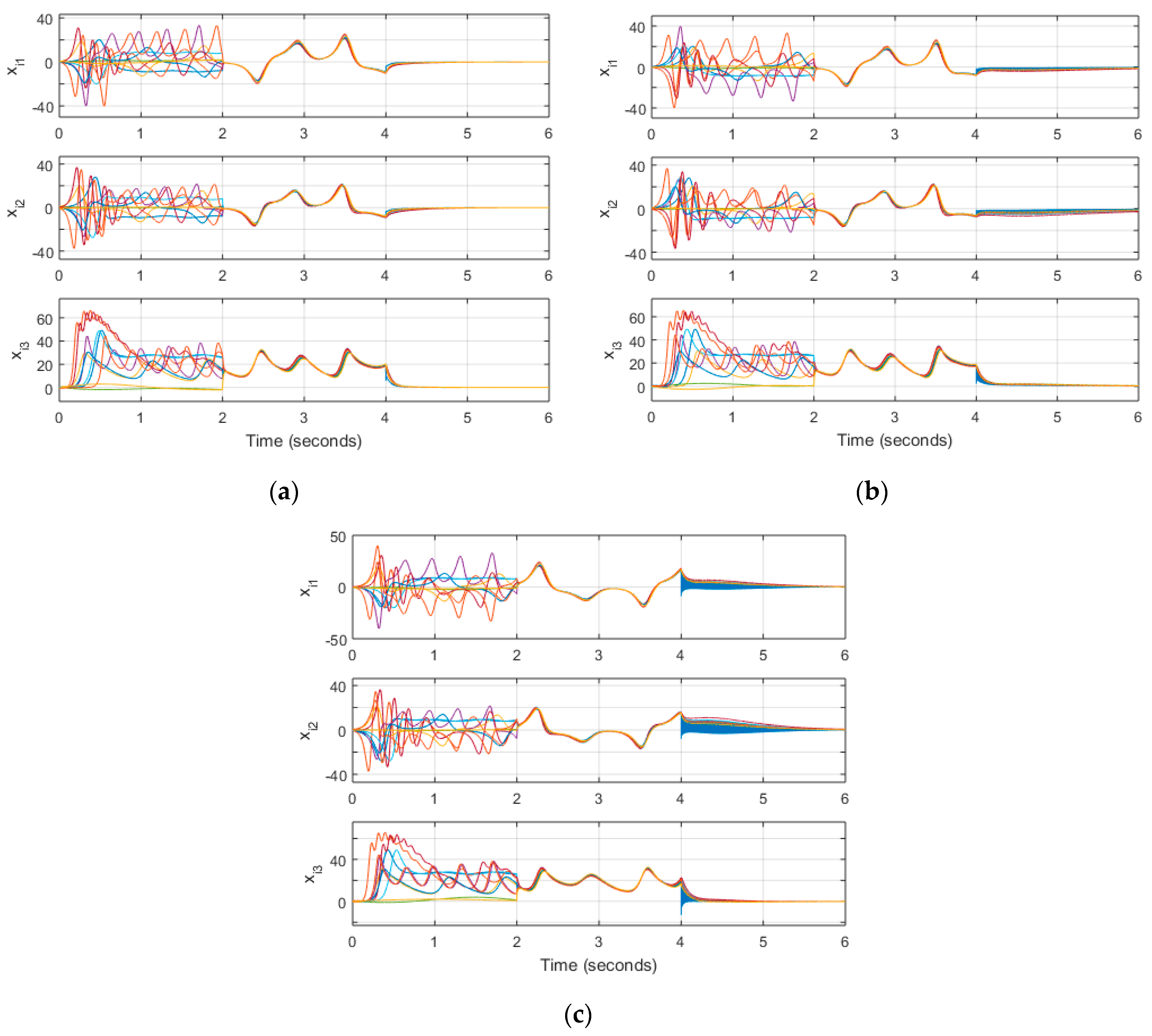
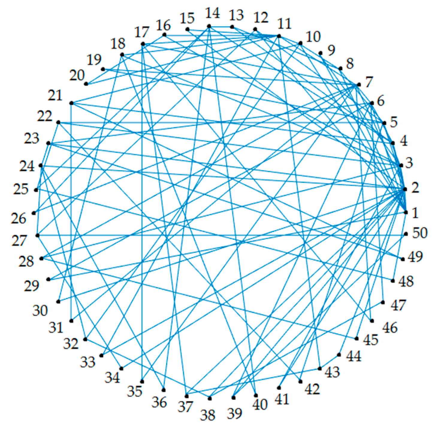
The same analysis was performed to the fifty-node network shown in Figure 14, with a connection strength $c=50$, and node self-dynamics appearing in the same order as past networks. V-stability analysis tells us that we need at least one controller for this network, but the bigger the network is, the harder it becomes to determine which node we should select to control. In order to facilitate the process, we select the three biggest nodes for control (nodes with the largest number of connections), these are 1, 2 and 7. With a gain $d_1=d_2=d_7=1000$ we can make the associated matrix $C$ negative definite. We apply this to the system that is continuous in discrete time and we increase the gain to $d_1=d_2=d_7=1500$ for the case where the control input is applied every 5T, and $d_1=d_2=d_7=2000$ for the case where the control input is applied every 10T. These results are shown in Figure 15. As before, we use the same RHONN structure as in past simulations.

Four additional topologies, illustrated in Figure 16, were simulated. New topologies consist of a five-node network with $c=25$, and a 13, 15, and 25 node networks with $c=100$. All of the node self-dynamics appear in the same order as past simulations. V-stability analysis for these topologies indicates that only one node is needed for control in all of them. Gains used are shown in

Table 2. Passivity degree values for the different chaotic systems.

Topology	Control Scheme	Gain	MSE	Variance
5 nodes	Input applied every time step	$d_3=300$	0.1498	0.1465
5 nodes	Input applied every 5T	$d_3=800$	4.9434	4.6425
5 nodes	Input applied every 10T	$d_3=1300$	2.8084	2.6858
13 nodes	Input applied every time step	$d_3=600$	0.3836	0.3451
13 nodes	Input applied every 5T	$d_3=1100$	8.2882	5.5867
13 nodes	Input applied every 10T	$d_3=1600$	14.1021	9.0395
15 nodes	Input applied every time step	$d_3=700$	3.7550	3.2386
15 nodes	Input applied every 5T	$d_3=1200$	9.3123	8.5676
15 nodes	Input applied every 10T	$d_3=1700$	34.5440	25.5843
25 nodes	Input applied every time step	$d_2=600$	1.0844	0.9308
25 nodes	Input applied every 5T	$d_2=1100$	3.4638	3.4205
25 nodes	Input applied every 10T	$d_2=1600$	9.7282	8.4571

Neural identification was implemented in every case using the same structure as explained in Section 6.

, where the subscript of $d$ indicates the pinned node, gains for the cases where the control input is applied at every time step are determined by the V-stability analysis, gains are increased for the rest of the cases. Starting from where the control input is applied (when time equals 4), to the end of the simulation (when time equals 6), mean square error and variance of all state elements of the network were obtained, and they are also presented in Table 2.

9. Conclusions

The concept of V-stability is studied and applied for a discrete-time complex network with continuous discrete-time and impulsive control schemes. A neural network was implemented as an identifier to synthesize the control law. The different control schemes were able to drive the system to state zero with some modifications made to analyze results in the case of the impulsive schemes. A formal rework of V-stability for impulsive complex networks may be a good research area as it proves to be a useful tool for continuous and continuous in discrete-time dynamical complex networks. One disadvantage of this method is the necessity to check eigenvalues of a given matrix, as the difficulty to do this increases as the network grows in size, although the 20-node network used here and some that are bigger are still manageable for unspecialized computer equipment.

In this work, we applied a novel neural-impulsive pinning control for complex networks for seven different topologies, each one with three different scenarios: input applied every time step, input applied every 5T, input applied every 10T, and the control design was carried out based on V-stability in order to stabilize the network states at zero, and all cases have an excellent evolution, as shown by the results presented in Section 7 and Section 8, showing the effectiveness of the proposed methodology for different complex network topologies with different dynamics in each node, without the need to apply control in every node at every time step.

An important area of application of the class of system considered in this paper is for biomedical purposes. Impulsive systems adapt well to how most of the treatments are administrated for different kind of diseases. In particular, a complex network approach, in this case, could represent the interaction between different individuals or a group of these people with specific relation to infectious diseases. These kinds of applications are considered as future work.