Efficient Computation of the Nonlinear Schrödinger Equation with Time-Dependent Coefficients


Abstract
1. Introduction
2. Theory
2.1. Explicit Runge–Kutta Pairs
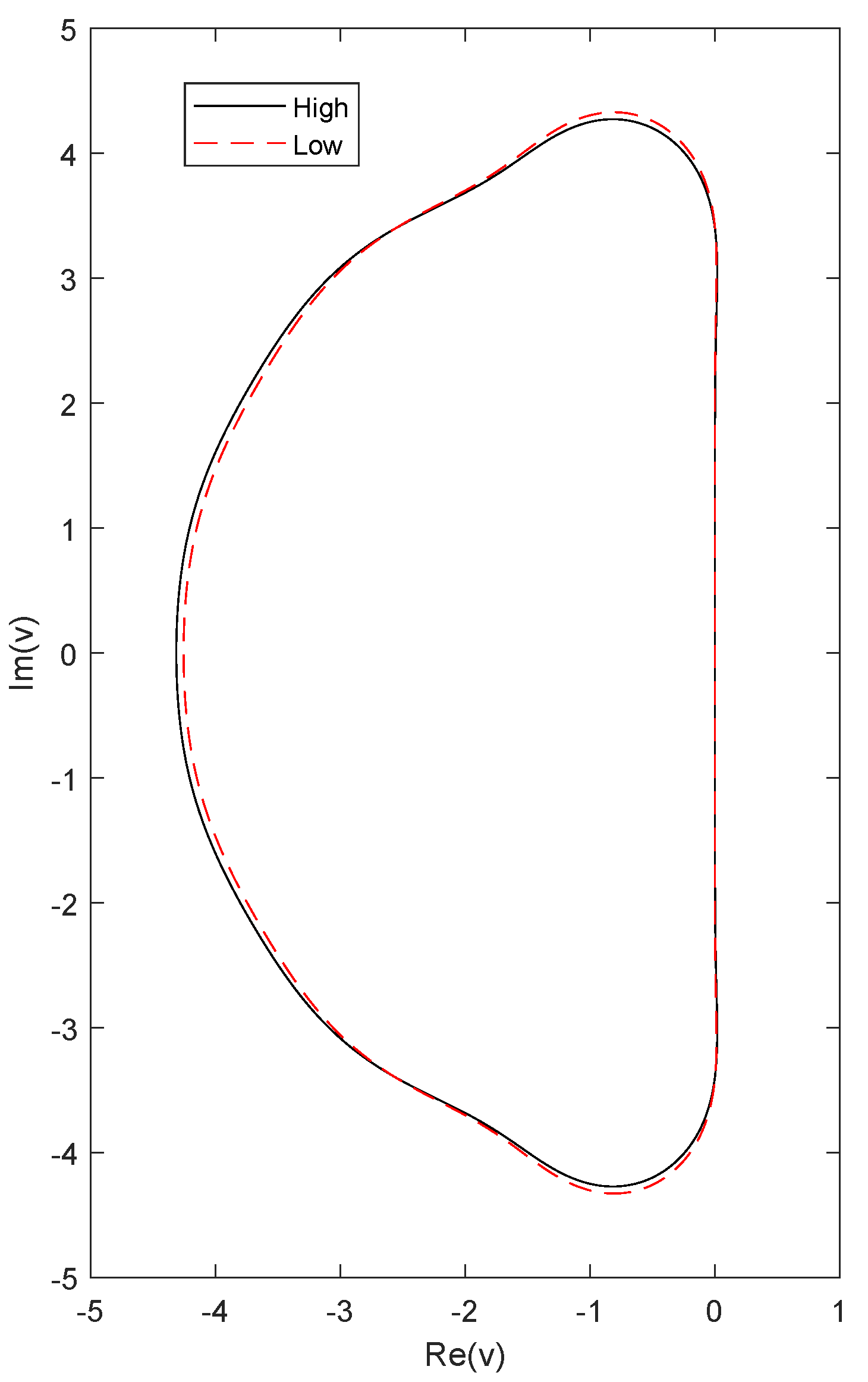
2.2. Phase-Lag and Stability
3. Construction and Analysis
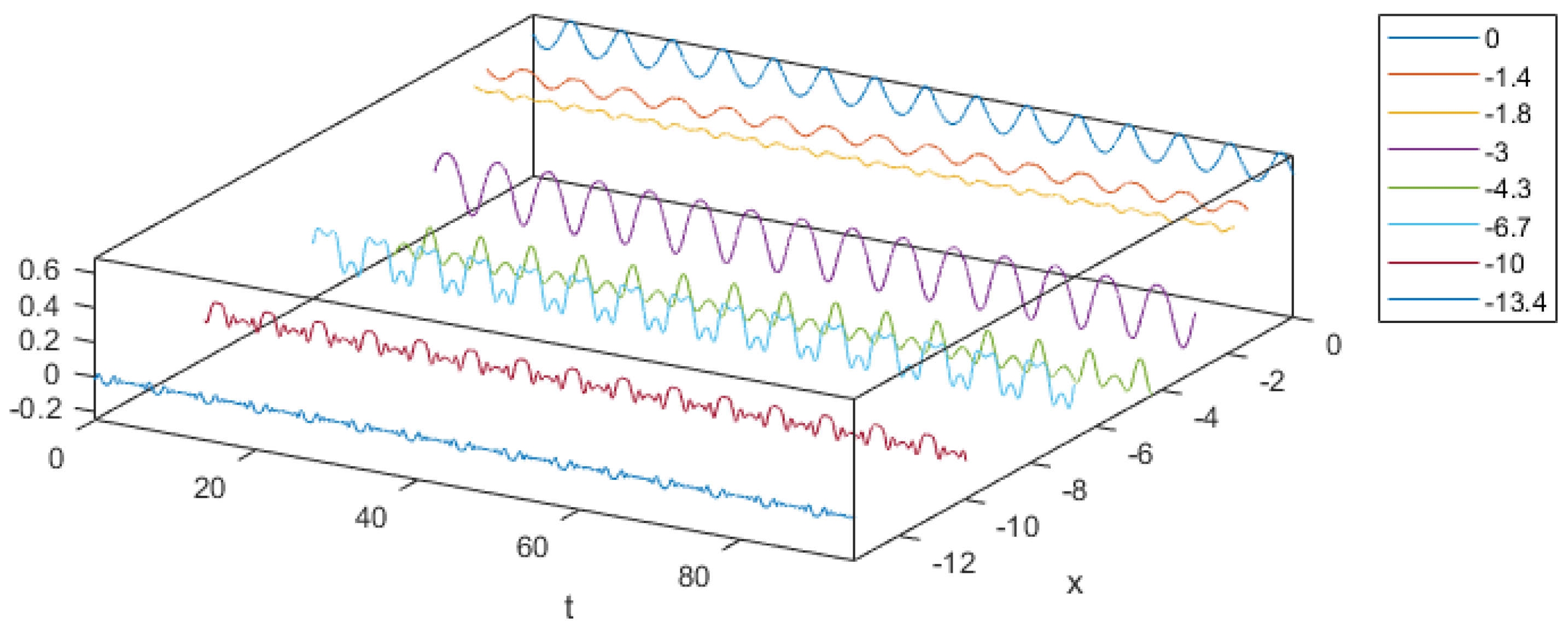
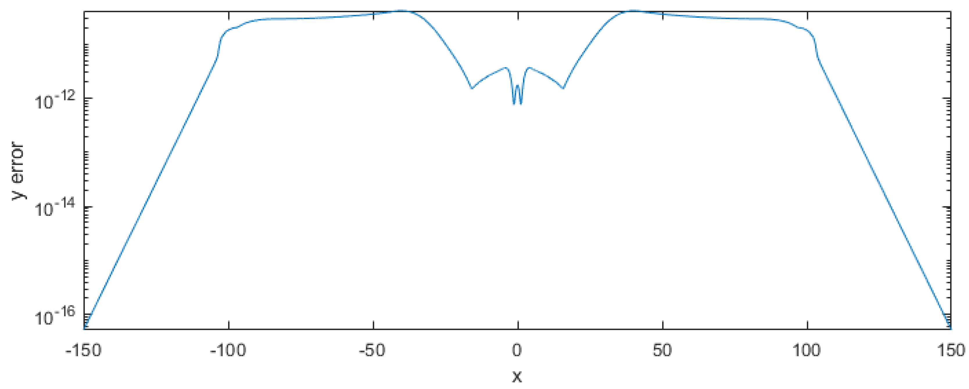
- Constant coefficients, since no dominant frequency exists for different values of x, as observed in Figure 1.
- Maximised phase-lag and amplification-error orders m and r of Definition 1, for improved behaviour when solving Equation (1) with periodic/oscillatory solutions.
- Maximised real stability interval, based on Definition 4.
- Coefficients with similar orders of magnitude, to minimise the round-off error.
- Low-order method with similar stability characteristics to the high-order one, to improve the local error estimation for extreme step sizes.
4. A Modified Step Size Control Algorithm
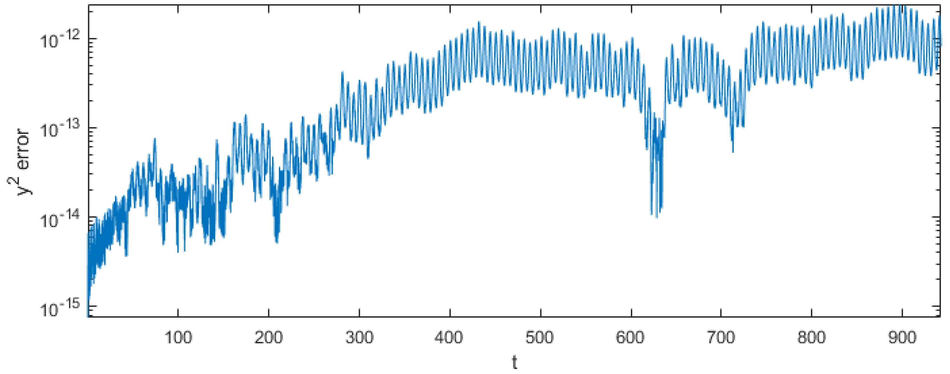
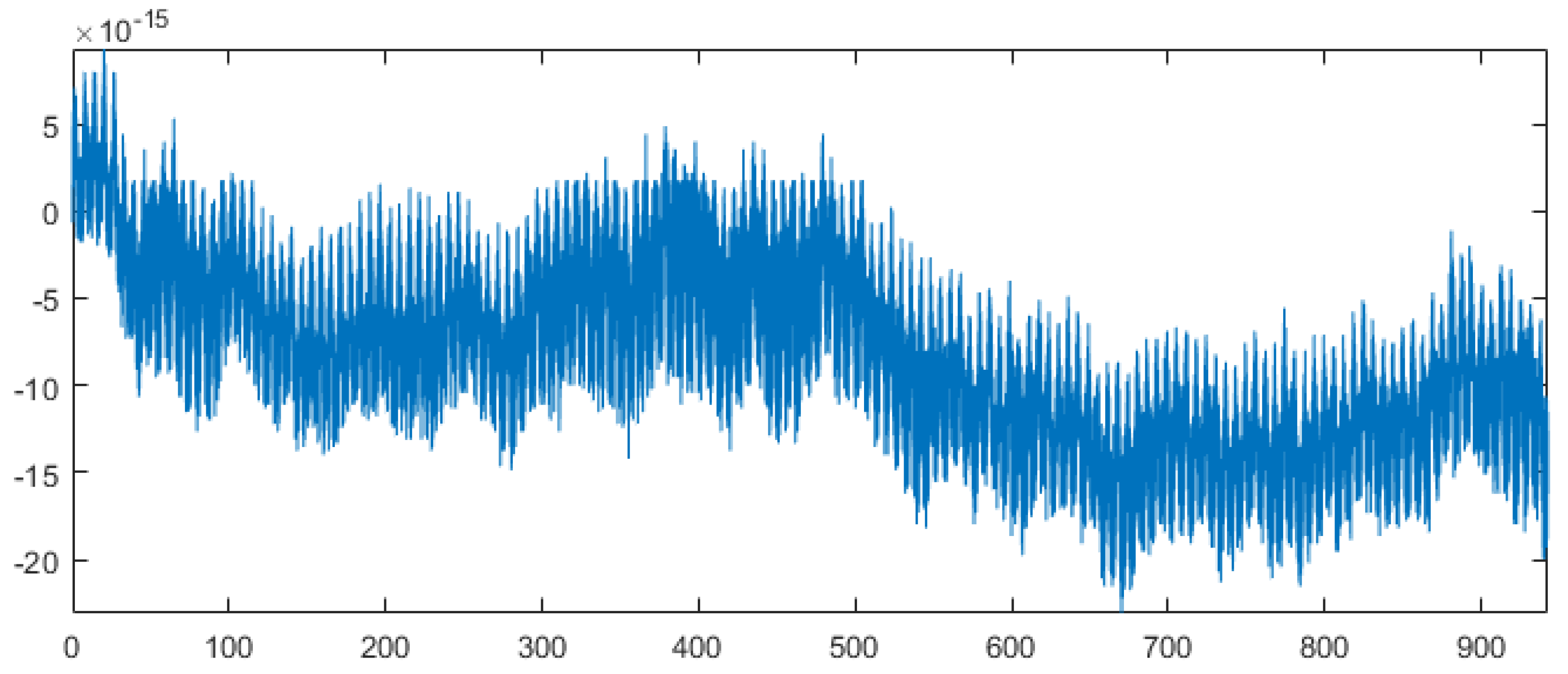
5. Numerical Experiments
5.1. Modified Step Size Control
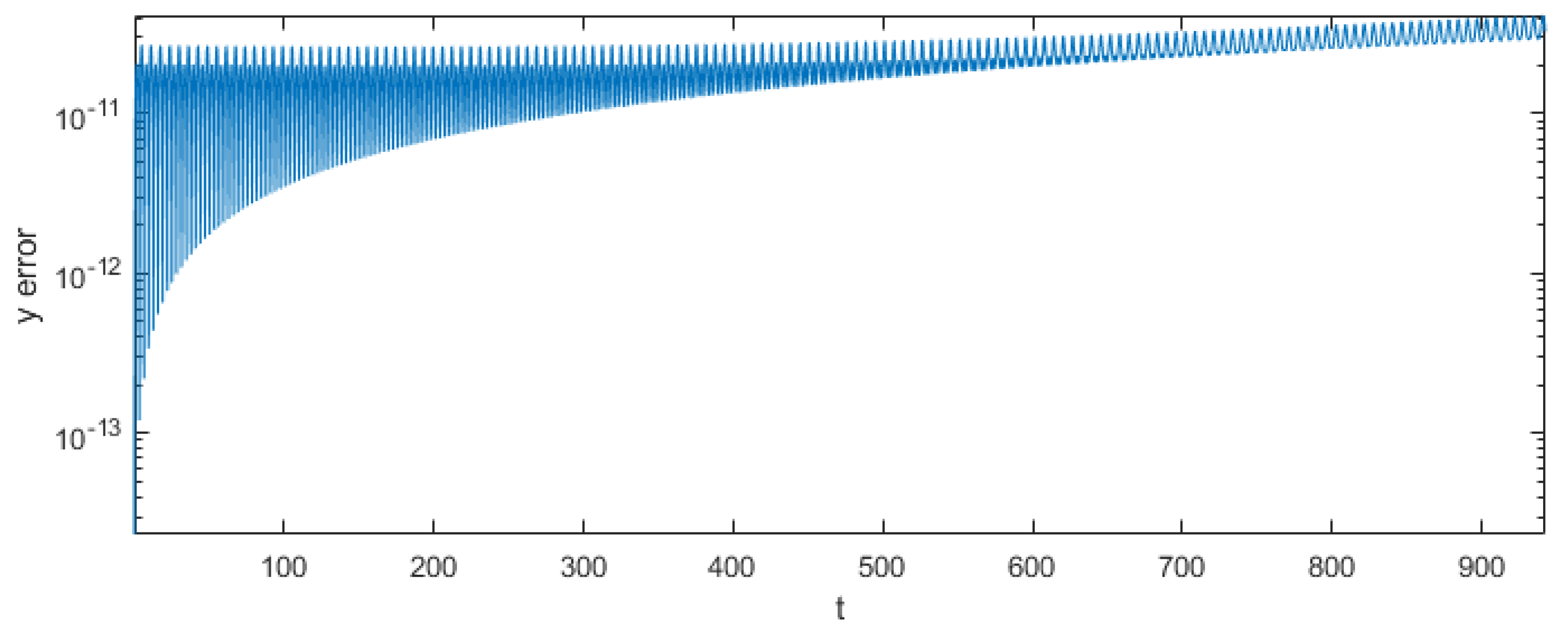
5.2. Results
6. Conclusions
Author Contributions
Funding
Acknowledgments
Conflicts of Interest
Notation
| Nonlinear Schrödinger equation | |
| mean-field matter wave function/complex electric field envelope | |
| t | time/propagation distance |
| x | longitudinal coordinate/transverse coordinate |
| dispersion | |
| nonlinearity | |
| global norm | |
| Runge–Kutta methods | |
| theoretical solution | |
| numerical solution | |
| h | step size |
| low and high algebraic orders | |
| , | low-order and high-order approximations of |
| Runge–Kutta coefficients | |
| Runge–Kutta coefficient matrices | |
| local error estimation | |
| tolerance | |
| Phase-lag and stability | |
| frequency | |
| stability polynomial | |
| imaginary stability interval | |
| real stability interval | |
References
- Moloney, J.V.; Newell, A.C. Nonlinear optics. Phys. D Nonlinear Phenom. 1990, 44, 1–37. [Google Scholar] [CrossRef]
- Pitaevskii, L.; Stringari, S. Bose-Einstein Condensation; Oxford University Press: Oxford, UK, 2003. [Google Scholar]
- Malomed, B. Multi-Component Bose-Einstein Condensates: Theory. In Emergent Nonlinear Phenomena in Bose-Einstein Condensates: Theory and Experiment; Springer: Berlin/Heidelberg, Germany, 2008; pp. 287–305. [Google Scholar] [CrossRef]
- Hong, J.; Liu, Y. A novel numerical approach to simulating nonlinear Schrödinger equations with varying coefficients. Appl. Math. Lett. 2003, 16, 759–765. [Google Scholar] [CrossRef]
- Zhong, W.P.; Belić, M.; Zhang, Y. Second-order rogue wave breathers in the nonlinear Schrödinger equation with quadratic potential modulated by a spatially-varying diffraction coefficient. Opt. Express 2015, 23, 3708–3716. [Google Scholar] [CrossRef] [PubMed]
- Kengne, E. Analytical solutions of nonlinear Schrödinger equation with distributed coefficients. Chaos Solitons Fractals 2014, 61, 56–68. [Google Scholar] [CrossRef]
- Amador, G.; Colon, K.; Luna, N.; Mercado, G.; Pereira, E.; Suazo, E. On Solutions for Linear and Nonlinear Schrödinger Equations with Variable Coefficients: A Computational Approach. Symmetry 2016, 8, 38. [Google Scholar] [CrossRef]
- Obaidat, S.; Mesloub, S. A New Explicit Four-Step Symmetric Method for Solving Schrödinger’s Equation. Mathematics 2019, 7, 1124. [Google Scholar] [CrossRef]
- Benia, Y.; Ruggieri, M.; Scapellato, A. Exact Solutions for a Modified Schrödinger Equation. Mathematics 2019, 7, 908. [Google Scholar] [CrossRef]
- Polyanin, A.D. Comparison of the Effectiveness of Different Methods for Constructing Exact Solutions to Nonlinear PDEs. Generalizations and New Solutions. Mathematics 2019, 7, 386. [Google Scholar] [CrossRef]
- Chen, J.; Zhang, Q. Ground State Solution of Pohozaev Type for Quasilinear Schrödinger Equation Involving Critical Exponent in Orlicz Space. Mathematics 2019, 7, 779. [Google Scholar] [CrossRef]
- Tsitoura, F.; Anastassi, Z.A.; Marzuola, J.L.; Kevrekidis, P.G.; Frantzeskakis, D.J. Dark solitons near potential and nonlinearity steps. Phys. Rev. A 2016, 94, 063612. [Google Scholar] [CrossRef]
- Lyu, P.; Vong, S. A linearized and second-order unconditionally convergent scheme for coupled time fractional Klein-Gordon-Schrödinger equation. Numer. Methods Partial Differ. Equ. 2018, 34, 2153–2179. [Google Scholar] [CrossRef]
- Jiang, C.; Cai, W.; Wang, Y. Optimal error estimate of a conformal Fourier pseudo-spectral method for the damped nonlinear Schrödinger equation. Numer. Methods Partial Differ. Equ. 2018, 34, 1422–1454. [Google Scholar] [CrossRef]
- Liao, F.; Zhang, L.; Hu, X. Conservative finite difference methods for fractional Schrödinger–Boussinesq equations and convergence analysis. Numer. Methods Partial Differ. Equ. 2019, 35, 1305–1325. [Google Scholar] [CrossRef]
- Malomed, B.A.; Stepanyants, Y.A. The inverse problem for the Gross–Pitaevskii equation. Chaos 2010, 20, 013130. [Google Scholar] [CrossRef]
- Serkin, V.N.; Hasegawa, A. Novel Soliton Solutions of the Nonlinear Schrödinger Equation Model. Phys. Rev. Lett. 2000, 85, 4502–4505. [Google Scholar] [CrossRef]
- Tang, C.; Zhang, F.; Yan, H.Q.; Chen, Z.Q.; Luo, T. Three-Step Predictor-Corrector of Exponential Fitting Method for Nonlinear Schrödinger Equations. Commun. Theor. Phys. 2005, 44, 435–439. [Google Scholar] [CrossRef]
- Kosti, A.A.; Anastassi, Z.A.; Simos, T.E. Construction of an optimized explicit Runge–Kutta–Nyström method for the numerical solution of oscillatory initial value problems. Comput. Math. Appl. 2011, 61, 3381–3390. [Google Scholar] [CrossRef]
- Kosti, A.A.; Anastassi, Z.A.; Simos, T.E. An optimized explicit Runge–Kutta–Nyström method for the numerical solution of orbital and related periodical initial value problems. Comput. Phys. Commun. 2012, 183, 470–479. [Google Scholar] [CrossRef]
- Anastassi, Z.A.; Kosti, A.A. A 6(4) optimized embedded Runge–Kutta–Nyström pair for the numerical solution of periodic problems. J. Comput. Appl. Math. 2015, 275, 311–320. [Google Scholar] [CrossRef]
- Kosti, A.A.; Anastassi, Z.A. Explicit almost P-stable Runge–Kutta–Nyström methods for the numerical solution of the two-body problem. Comput. Appl. Math. 2015, 34, 647–659. [Google Scholar] [CrossRef]
- Demba, M.; Senu, N.; Ismail, F. A 5(4) Embedded Pair of Explicit Trigonometrically-Fitted Runge–Kutta–Nyström Methods for the Numerical Solution of Oscillatory Initial Value Problems. Math. Comput. Appl. 2016, 21, 46. [Google Scholar] [CrossRef]
- Ahmad, N.A.; Senu, N.; Ismail, F. Phase-Fitted and Amplification-Fitted Higher Order Two-Derivative Runge-Kutta Method for the Numerical Solution of Orbital and Related Periodical IVPs. Math. Probl. Eng. 2017, 2017, 1871278. [Google Scholar] [CrossRef]
- Simos, T.E.; Papakaliatakis, G. Modified Runge–Kutta Verner methods for the numerical solution of initial and boundary-value problems with engineering applications. Appl. Math. Model. 1998, 22, 657–670. [Google Scholar] [CrossRef]
- Tsitouras, C.; Simos, T.E. Optimized Runge–Kutta pairs for problems with oscillating solutions. J. Comput. Appl. Math. 2002, 147, 397–409. [Google Scholar] [CrossRef]
- Triantafyllidis, T.V.; Anastassi, Z.A.; Simos, T.E. Two optimized Runge-Kutta methods for the solution of the Schrödinger equation. MATCH Commun. Math. Comput. Chem. 2008, 60, 3. [Google Scholar]
- Kosti, A.A.; Anastassi, Z.A.; Simos, T.E. An optimized explicit Runge-Kutta method with increased phase-lag order for the numerical solution of the Schrödinger equation and related problems. J. Math. Chem. 2010, 47, 315. [Google Scholar] [CrossRef]
- Papageorgiou, G.; Tsitouras, C.; Papakostas, S.N. Runge-Kutta pairs for periodic initial value problems. Computing 1993, 51, 151–163. [Google Scholar] [CrossRef]
- Berland, J.; Bogey, C.; Bailly, C. Low-dissipation and low-dispersion fourth-order Runge–Kutta algorithm. Comput. Fluids 2006, 35, 1459–1463. [Google Scholar] [CrossRef]
- Tsitouras, C. A parameter study of explicit Runge-Kutta pairs of orders 6(5). Appl. Math. Lett. 1998, 11, 65–69. [Google Scholar] [CrossRef]
- Shampine, L.F. Error estimation and control for ODEs. J. Sci. Comput. 2005, 25, 3–16. [Google Scholar] [CrossRef]
- Auzinger, W.; Kassebacher, T.; Koch, O.; Thalhammer, M. Adaptive splitting methods for nonlinear Schrödinger equations in the semiclassical regime. Numer. Alg. 2016, 72, 1–35. [Google Scholar] [CrossRef]
- Auzinger, W.; Hofstätter, H.; Koch, O.; Thalhammer, M. Defect-Based Local Error Estimators for Splitting Methods, with Application to Schrödinger Equations, Part III. J. Comput. Appl. Math. 2015, 273, 182–204. [Google Scholar] [CrossRef]
- Thalhammer, M.; Abhau, J. A numerical study of adaptive space and time discretisations for Gross–Pitaevskii equations. J. Comput. Phys. 2012, 231, 6665–6681. [Google Scholar] [CrossRef] [PubMed]
- Balac, S.; Fernandez, A. Mathematical analysis of adaptive step-size techniques when solving the nonlinear Schrödinger equation for simulating light-wave propagation in optical fibers. Opt. Commun. 2014, 329, 1–9. [Google Scholar] [CrossRef][Green Version]
- Butcher, J.C. Trees and numerical methods for ordinary differential equations. Numer. Alg. 2010, 53, 153–170. [Google Scholar] [CrossRef]
- Popelier, P.L.; Simos, T.E.; Wilson, S. Chemical Modelling: Applications and Theory; Royal Society of Chemistry: London, UK, 2000; Volume 1. [Google Scholar]


| 0 | ||||||||
| 1 | ||||||||
| b | 0 | 0 | ||||||
| 0 | ||||||||
| H(L)S | PL | AE | IR | II | |
|---|---|---|---|---|---|
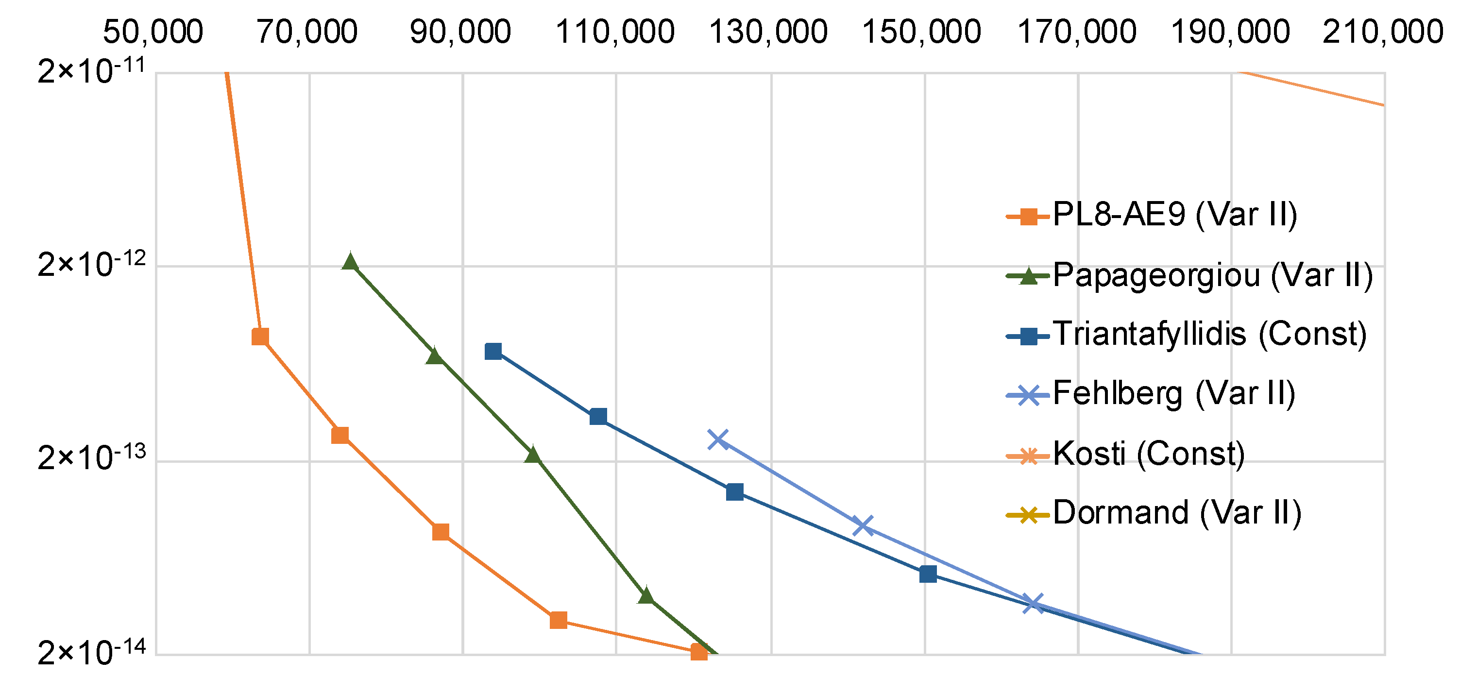
| PL8-AE9 (Table 1) | 6(4)8 | 8 | 9 | −4.31 | 3.39 |
| Papageorgiou [29] | 6(5)8 | 10 | 11 | −4.51 | 3.06 |
| Triantafyllidis [27] | 6(-)8 | 10 | 7 | −4.51 | 3.06 |
| Fehlberg [37] | 6(5)8 | 6 | 7 | −4.06 | 1.30 |
| Kosti [28] | 5(-)6 | 8 | 5 | −3.83 | 0.002 |
| Dormand [37] | 5(4)7 | 6 | 5 | −3.30 | 0.99 |
© 2020 by the authors. Licensee MDPI, Basel, Switzerland. This article is an open access article distributed under the terms and conditions of the Creative Commons Attribution (CC BY) license (http://creativecommons.org/licenses/by/4.0/).
Share and Cite
Kosti, A.A.; Colreavy-Donnelly, S.; Caraffini, F.; Anastassi, Z.A. Efficient Computation of the Nonlinear Schrödinger Equation with Time-Dependent Coefficients. Mathematics 2020, 8, 374. https://doi.org/10.3390/math8030374
Kosti AA, Colreavy-Donnelly S, Caraffini F, Anastassi ZA. Efficient Computation of the Nonlinear Schrödinger Equation with Time-Dependent Coefficients. Mathematics. 2020; 8(3):374. https://doi.org/10.3390/math8030374
Chicago/Turabian StyleKosti, Athinoula A., Simon Colreavy-Donnelly, Fabio Caraffini, and Zacharias A. Anastassi. 2020. "Efficient Computation of the Nonlinear Schrödinger Equation with Time-Dependent Coefficients" Mathematics 8, no. 3: 374. https://doi.org/10.3390/math8030374
APA StyleKosti, A. A., Colreavy-Donnelly, S., Caraffini, F., & Anastassi, Z. A. (2020). Efficient Computation of the Nonlinear Schrödinger Equation with Time-Dependent Coefficients. Mathematics, 8(3), 374. https://doi.org/10.3390/math8030374