Meshless Analysis of Nonlocal Boundary Value Problems in Anisotropic and Inhomogeneous Media

Abstract

In this work, meshless methods based on a radial basis function (RBF) are applied for the solution of two-dimensional steady-state heat conduction problems with nonlocal multi-point boundary conditions (NMBC). These meshless procedures are based on the multiquadric (MQ) RBF and its modified version (i.e., integrated MQ RBF). The meshless method is extended to the NMBC and compared with the standard collocation method (i.e., Kansa’s method). In extended methods, the interior and the boundary solutions are approximated with a sum of RBF series, while in Kansa’s method, a single series of RBF is considered. Three different sorts of solution domains are considered in which Dirichlet or Neumann boundary conditions are specified on some part of the boundary while the unknown function values of the remaining portion of the boundary are related to a discrete set of interior points. The influences of NMBC on the accuracy and condition number of the system matrix associated with the proposed methods are investigated. The sensitivity of the shape parameter is also analyzed in the proposed methods. The performance of the proposed approaches in terms of accuracy and efficiency is confirmed on the benchmark problems.

1. Introduction

The partial differential equations with nonlocal boundary conditions that emerged in the literature have significant applications in the fields of engineering, astrophysics, and biology. Some of the first nonlocal equations that appeared in the literature are encountered in the field of phase transition and are related to theories due to Van der Waals, Ginzburg, Landau, and Cahn & Hilliard [1]. For instance, such models with nonlocal spatial terms are encountered in the Ohmic heating production [2], in the shear banding formation in metals being deformed under high strain rates [3,4], in the theory of gravitational equilibrium of polytropic stars [5], in the investigation of the fully turbulent behavior of real flows, using invariant measures for the Euler equation [6], in population dynamics [7], in modeling aggregation of cells via interaction with a chemical substance (chemotaxis) [8], and in image processing [9].

Therefore, nonlocality is not a technical obstruction to scientific research but it provides the essence of what happens in reality, and for that purpose, its mathematical study can provide very useful predictions in many areas of applications. In general, nonlocal models provide more accurate predictions compared to their local counterparts since they use all the available information regarding the evolution of the inspected process.

Nonlocal boundary conditions have significant applications in engineering and biological sciences. These nonlocal boundary conditions arise in mathematical models of various biological, physical, and chemical processes. In addition, nonlocal boundary conditions also have wide applications in heat conduction processes, control theory, chemical diffusion, population dynamics, blood flow problems, underground water flow, and chemical engineering. Related references and examples of mathematical models involving nonlocal boundary conditions can be found in [10,11,12,13,14,15]. Nonlocal boundary value problems arise when the boundary values of the solution are not known on the boundaries. In such circumstances, the solution at the boundaries is connected with the solution inside the given domain. This type of formulation is placed in a separate class known as nonlocal boundary value problems.

It is sometimes better to impose nonlocal boundary conditions since the measurements needed by a nonlocal boundary condition may be more precise than the measurement given by a local condition. For example, consider the second order differential equation [12]

$$u^{″}\left(t\right)=g(t,u\left(t\right),u^{\prime }\left(t\right)),$$

(1)

subject to local boundary conditions

$$u\left(0\right)=0,u^{\prime }\left(1\right)=0.$$

(2)

Equation (2) is called a mixed type boundary condition because on $t=0$, u is prescribed and the derivative is prescribed on $t=1$. Since we know that, in the process of numerical computation and a scientific experiment, the value of $u^{\prime }\left(1\right)$ is more difficult to determine than that of $\frac{u\left(\xi \right)-u\left(1\right)}{\xi -1}$ where $(0<\xi <1)$; therefore, by replacing $u^{\prime }\left(1\right)$ in (2) with $\frac{u\left(\xi \right)-u\left(1\right)}{\xi -1}$ we have nonlocal boundary conditions:

$$u\left(0\right)=0,u\left(1\right)=u\left(\xi \right).$$

(3)

Equation (1) along with (3) is called a nonlocal boundary value problem. Equation (3) is called two-point boundary condition which is a special type of multi-point boundary condition.

Meshless methods for the solutions of differential equations are being successfully applied in various fields of science and engineering; therefore, they are more effective and suitable for complex domains as compared to mesh-based numerical methods. Since a set of independent points is required for meshless methods, they are often better suited for complex geometries. The computational costs associated with mesh generation in mesh-based methods are high [16] as compared to meshless methods. In comparison to meshless methods, other traditional numerical methods such as finite difference methods, finite element methods, and finite volume methods are usually limited to problems involving two or three spacial variables (space dimensions).

Literature suggests that multiquadric (MQ) RBF is considered the best in accuracy among different types of RBFs; however, the shape of the function is controlled by shape parameter $ϵ$. The $ϵ$ effects the accuracy of the method where its optimal value can lead to good approximations. To determine the optimal value of the $ϵ$ is an open problem and there is no such mathematical theory developed for optimal value of $ϵ$. Another drawback is the high condition number of the interpolation matrix. The ill-conditional system matrix arises in the case of globally supported RBFs, as the separation distance $\frac{1}{2}{max}_{i\ne j}{\parallel x_i-x_j\parallel }_2,i,j=1,2,3,...,N,$ between data points decreases for fixed values of the shape parameter $ϵ$ [17]. Many prominent researchers have used a different value of the shape parameter in the hope of accurately handling such problems. Both constant and variable shape parameters are recommended. Hardy introduced the following shape parameter formula in [18]:

$$ϵ=\frac{0.815{\sum }_{j=1}^N{d}_j}{N},$$

where N is number of collocation points and $d_j$ is the distance from the jth center to its nearest neighbor. Later on, a smallest circle enclosing all data points is considered and the shape parameters ($ϵ=\frac{1.25}{\sqrt{N}}\times \mathrm{diameter}\mathrm{of}\mathrm{this}\mathrm{circle}$) were recommended in [19]. The shape parameter $\frac{2}{\sqrt{N}}$ was used for solution of nonlinear PDEs in [20]. In [21], two optimal values of the shape parameter 1.03 and 1.42 were recommended for MQ RBF, whereas for Gaussian basis, a range $0.003–0.03$ was given, for solving cantilever beam and perforated strip plate problems. In [11,22,23], it is concluded that splitting of shape parameter into x- and y-axes give good results, i.e., ${ϵ}_x=h_x{N}_x^2$ and ${ϵ}_y=h_y{N}_y^2$, where $h_x$ and $h_y$ are positive constants, but the condition number of the collocation matrix is high. Different selection procedures of shape parameter can also be found in [24,25,26,27,28,29,30,31,32].

In this paper, a meshless discretization technique based on MQ RBF and its modified form, i.e., integrated MQ RBF, is applied for the numerical solution of elliptic PDEs with nonlocal boundary conditions (NBC). In the last few decades, the RBF-based collocation technique for the solution of nonlocal boundary value problems has been a vital research area in many branches of science and hence was successfully applied to solve such problems numerically [33,34,35]. A one-dimensional hyperbolic equation with an integral boundary condition was studied in [36]. The two-dimensional diffusion equation subject to a nonlocal condition involving a double integral along with Neumann’s boundary conditions was formulated in a rectangular region. Such a problem is solved numerically using a meshless collocation method [37]. In paper [38], the RBF-based collocation technique was also applied to investigate the influences of nonlocal conditions on the optimal selection of shape parameter $ϵ$, ill-conditioning, and accuracy of the method. A nonlocal, two-dimensional Poisson equation was solved with two-point and integral boundary conditions; it was formulated on one side of the rectangular region. Later, in [11], a comparison of the RBF-based collocation technique with the Haar wavelet-based collocation technique was studied for the same problem. Due to the splitting of the shape parameter into x and y directions, its distribution effect on the accuracy of the problem at hand was also investigated. The influences of shape parameter $ϵ$ and the distribution of nodes on the accuracy of the RBF-based collocation technique were investigated by considering the multidimensional linear elliptic equation with integral conditions [39]. Recently, the RBF-based meshless method has been applied to elliptic PDEs with nonlocal multi-point boundary conditions (NMBC) [40].

It is known that the meshless method can be successfully applied to solve such nonlocal problems. However, it was shown (e.g., see paper [11,38,40]) that due to the nonlocal parameter $\gamma$, the condition number $\kappa$ of the system matrix involved and accuracy of the method are affected. It is shown that the RBF-based collocation technique gives quite good results for the optimal value of shape parameter [38,40]. On the other hand, for the optimal value of the shape parameter, the accuracy and conditioning are also slightly affected by NBC. This paper aims to investigate the effect of this parameter on the property of the RBF-based method using integrated MQ RBF.

Furthermore, some other applications of RBF are successfully implemented for parabolic and elliptic interface problems [41,42,43], highly oscillatory integral equations [44,45,46,47,48,49], stokes equations with interface conditions [50], and time-dependent PDEs [51].

Nowadays, integrated RBF(s) are successfully implemented in solving miscellaneous differential equations. An MQ RBF integrated twice with a fixed value of shape parameter $ϵ$ was used by [52] to solve one-dimensional problems. Elliptic problems were solved by [53] through a multi-domain integrated RBF collocation method. Higher-order ODEs and PDEs were solved by an integrated RBF method in the papers [54,55]. Further detail about integrated RBFs can be found in [17,56,57,58].

We have implemented four different methods based on radial basis functions, i.e., the Kansa method (multi-quadric is a basis function) and the Kansa method (integrated-multi quadric is a basis function), and we extended the method proposed in [59] (with these two different basis functions) to the complicated nonlocal boundary value problems. For the first time, these methods were applied to the nonlocal Neumann boundary value problems accurately, which can be very complicated in the case of finite difference and finite element methods. An accurate numerical approximation for the unknown boundary function has been obtained through these techniques.

The paper is distributed into five sections, including the present introductory Section 1. In Section 2, we discuss the governing equations along with different types of boundary conditions. In Section 3, the numerical procedure is described. Numerical experiments are given in Section 4. Some conclusions are drawn in Section 5.

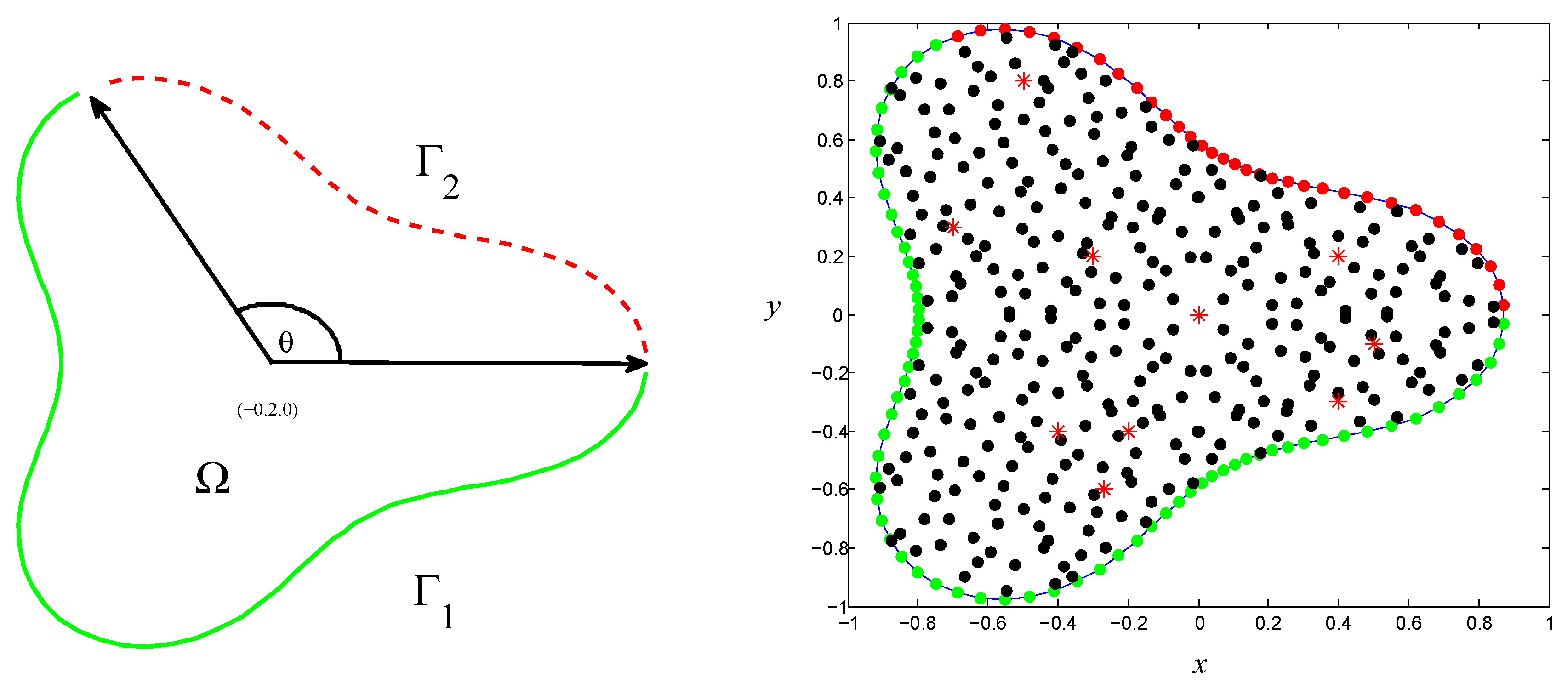
2. Governing Equation

A general form of the diffusion equation is given by [59]

$$\begin{array}{cc}\hfill & k_{1,1}\left(\widehat{\mathbf{v}}\right)\frac{{\partial }^2}{\partial x^2}u\left(\widehat{\mathbf{v}}\right)+2k_{1,2}\left(\widehat{\mathbf{v}}\right)\frac{{\partial }^2}{\partial x\partial y}u\left(\widehat{\mathbf{v}}\right)+k_{2,2}\left(\widehat{\mathbf{v}}\right)\frac{{\partial }^2}{\partial y^2}u\left(\widehat{\mathbf{v}}\right)+\left(\frac{\partial }{\partial x}{k}_{1,1}\left(\widehat{\mathbf{v}}\right)+\frac{\partial }{\partial y}{k}_{1,2}\left(\widehat{\mathbf{v}}\right)\right)\frac{\partial }{\partial x}u\left(\widehat{\mathbf{v}}\right)+\hfill \\ \hfill & \left(\frac{\partial }{\partial x}{k}_{1,2}\left(\widehat{\mathbf{v}}\right)+\frac{\partial }{\partial y}{k}_{2,2}\left(\widehat{\mathbf{v}}\right)\right)\frac{\partial }{\partial y}u\left(\widehat{\mathbf{v}}\right)=f\left(\widehat{\mathbf{v}}\right),\widehat{\mathbf{v}}=(x,y)\in \mathsf{\Omega }.\hfill \end{array}$$

(4)

The above model is subject to mixed boundary conditions:

• Classical Dirichlet boundary conditions:

  $$u\left(\widehat{\mathbf{v}}\right)=g\left(\widehat{\mathbf{v}}\right),\widehat{\mathbf{v}}\in {\mathsf{\Gamma }}_1.$$

  (5)
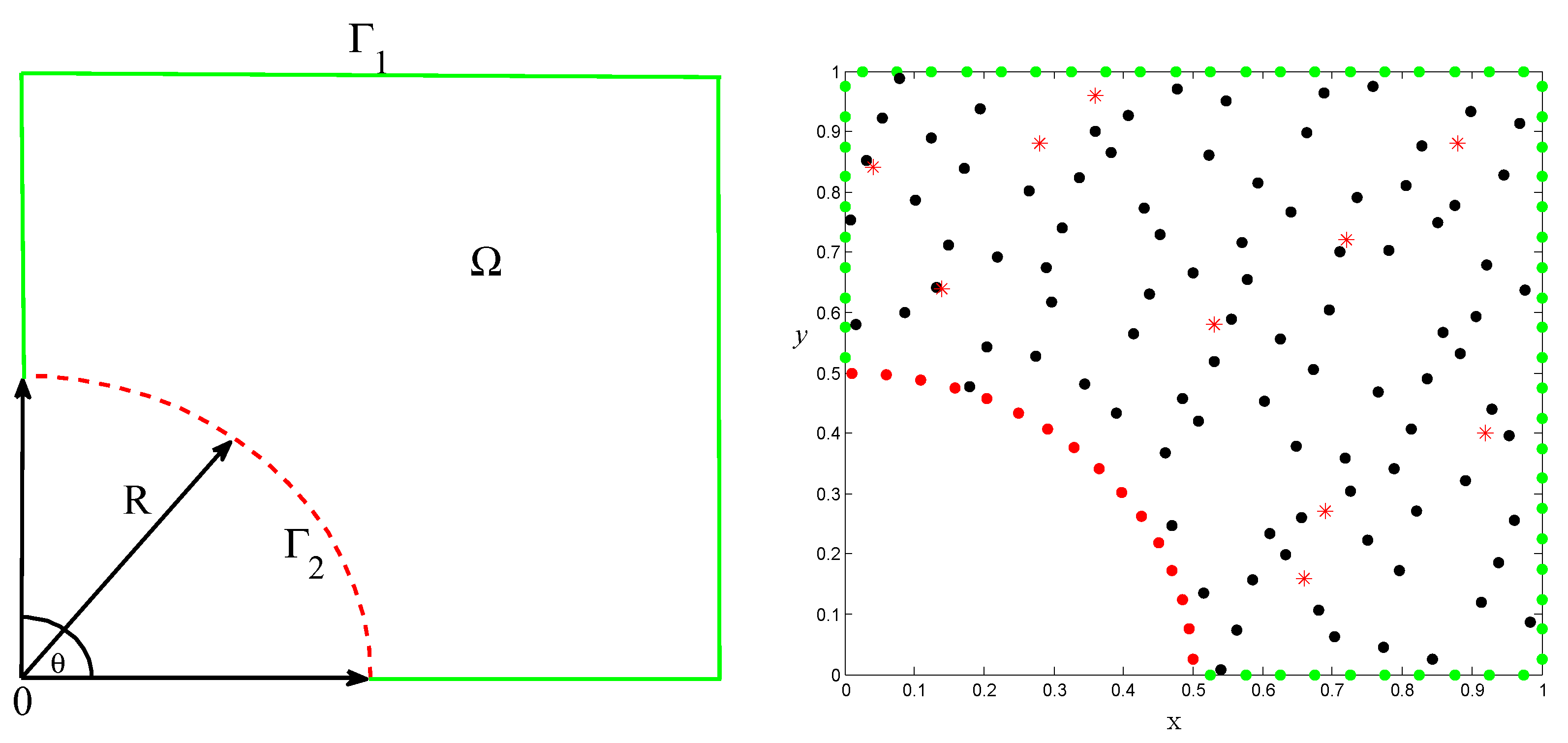
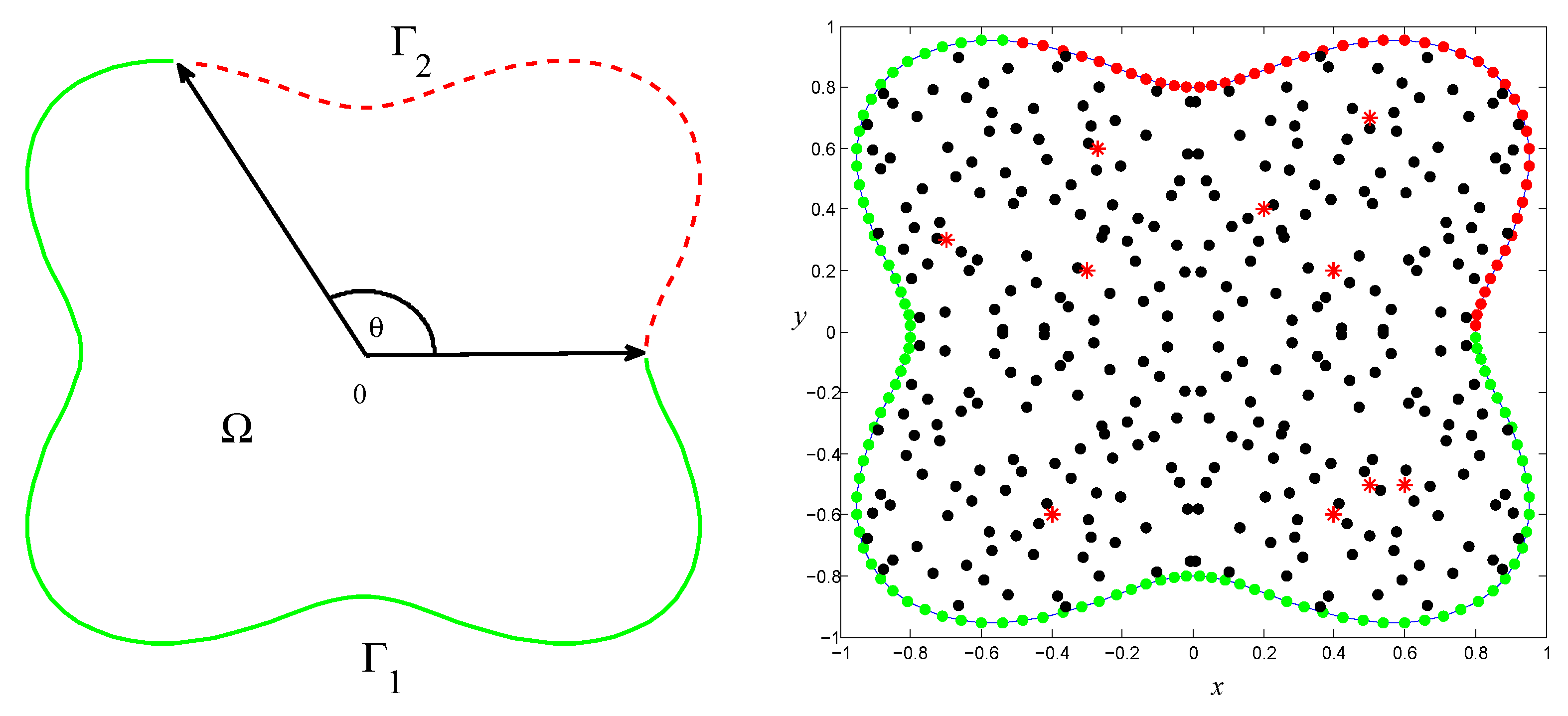
• • Nonlocal multipoint boundary conditions:

  $$u\left(\widehat{\mathbf{v}}\right)-\sum _{l=1}^n\gamma u\left({\widehat{\mathbf{v}}}_l^{★}\right)=h\left(\widehat{\mathbf{v}}\right),\widehat{\mathbf{v}}\in {\mathsf{\Gamma }}_2,{\widehat{\mathbf{v}}}^{★}\in {\mathsf{\Omega }}^{★},$$

  (6)

  where ${\mathsf{\Omega }}^{★}\subset \mathsf{\Omega }$ are set of discrete distinct scattered points inside the solution domain and n is the number of these scattered points. Throughout the paper we will take $n=10$; if not, it will be mentioned. It is also assumed that the distribution of the points ${\widehat{\mathbf{v}}}_l^{★}$ on the solution domain will be fixed. The given functions are $k_{1,1}$, $k_{1,2}$, $k_{2,2}$, f, g, h, and the parameter $\gamma$. $\mathsf{\Omega }$ is the interior portion of the solution domain and $\mathsf{\Gamma }={\mathsf{\Gamma }}_1\cup {\mathsf{\Gamma }}_2$ are the boundary parts of the solution domain such that ${\mathsf{\Gamma }}_1\cap {\mathsf{\Gamma }}_2=\varnothing$ and ${\mathsf{\Gamma }}_2\ne \varnothing$. The NBC defined on the boundary ${\mathsf{\Gamma }}_2$ is reduced to Dirichlet boundary condition when $\gamma =0$.

3. The Numerical Scheme

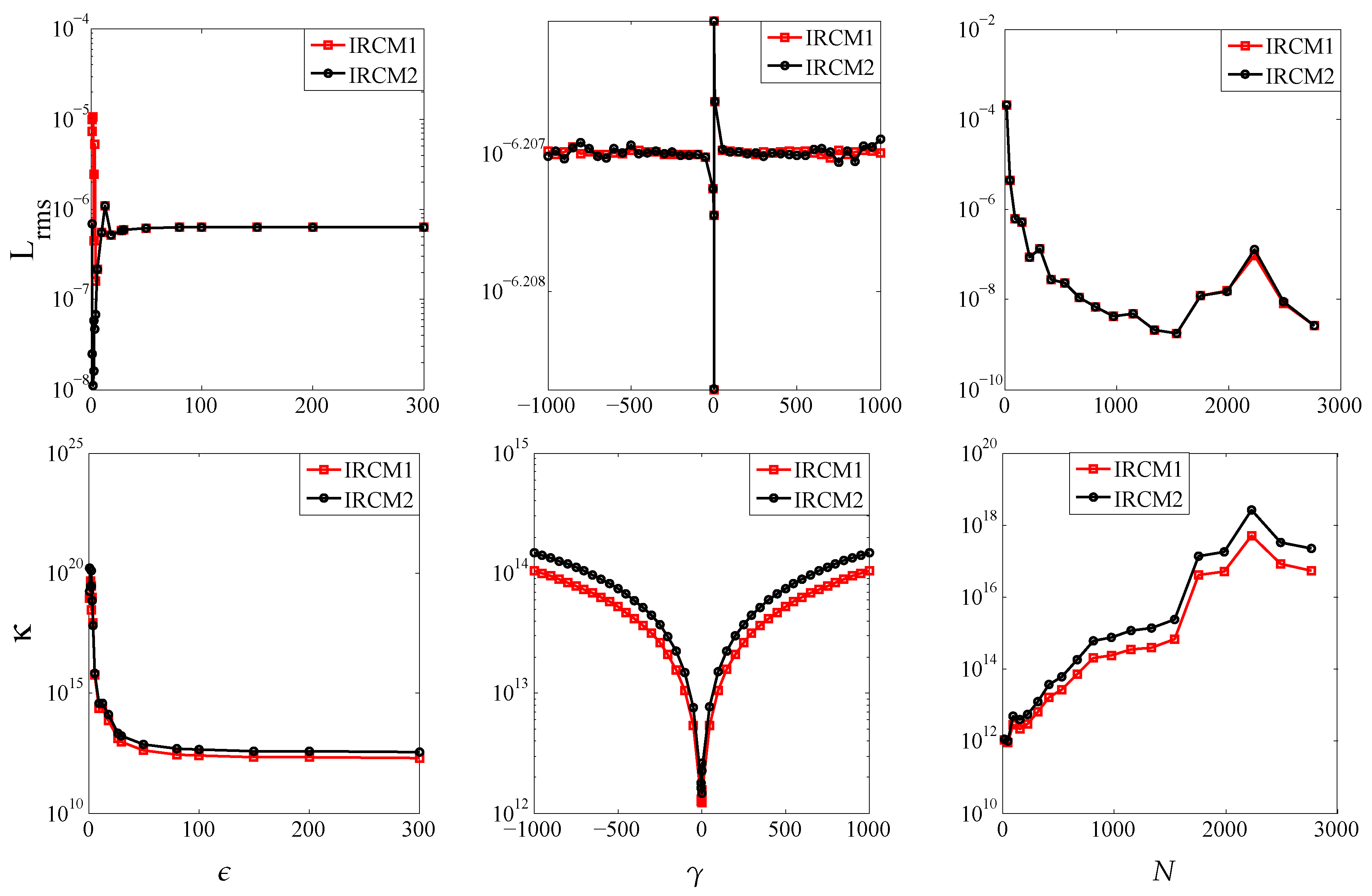
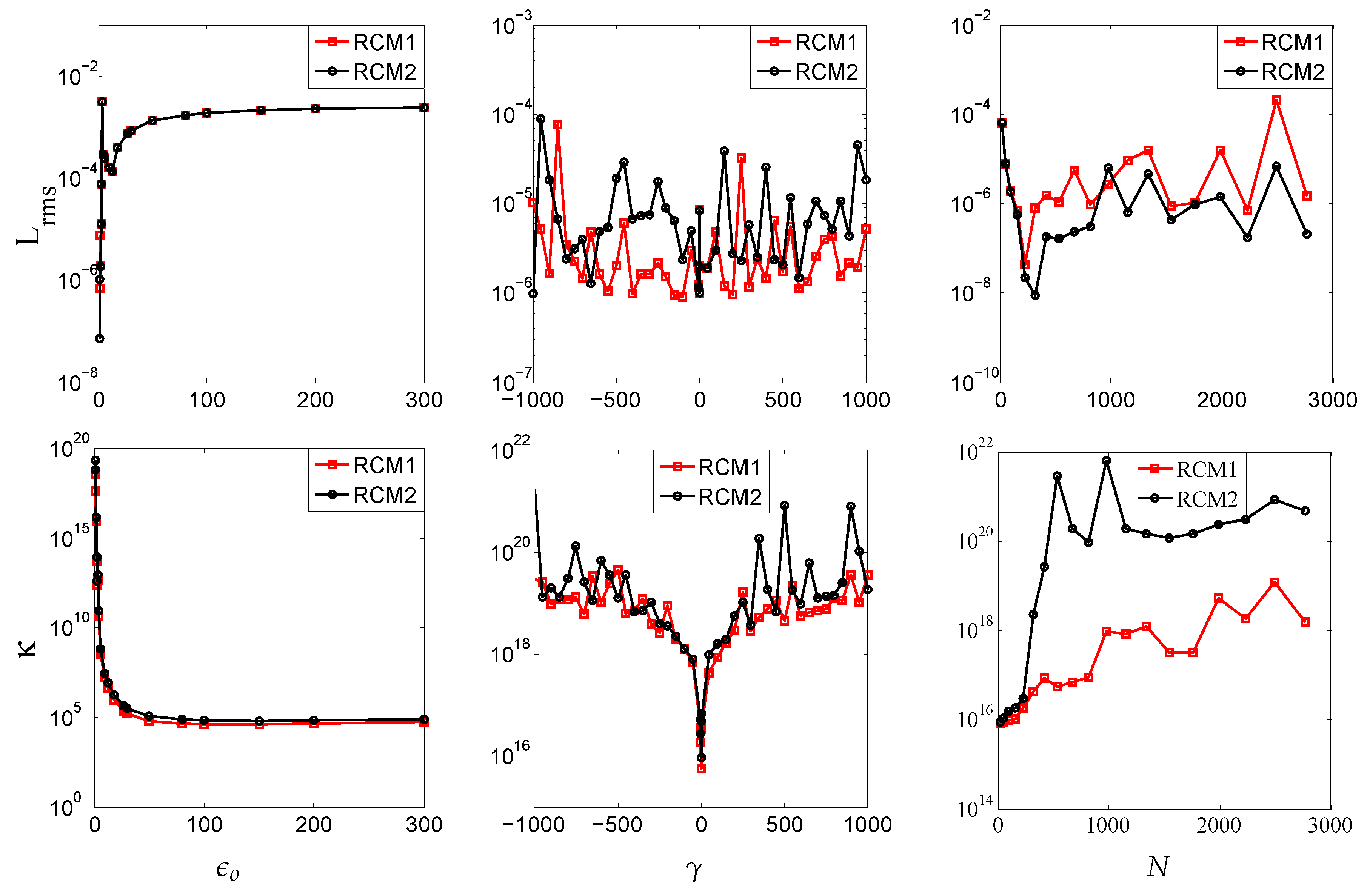
Let us divide the solution domain into three disjoint sets. The set of inner distinct scattered nodes:

$$\widehat{\mathsf{\Omega }}={\{(x_j,y_j)\}}_{j=1}^N,$$

(7)

and the set of distinct scattered boundary points:

$${\widehat{\mathsf{\Gamma }}}_1={\{(x_{l_1},y_{l_1})\}}_{l_1=1}^{M_1},$$

(8)

$${\widehat{\mathsf{\Gamma }}}_2={\{(x_{l_2},y_{l_2})\}}_{l_2=1}^{M_2},$$

(9)

such that $\widehat{\mathsf{\Omega }}\subset \mathsf{\Omega }$, ${\widehat{\mathsf{\Gamma }}}_1\subset {\mathsf{\Gamma }}_1$, and ${\widehat{\mathsf{\Gamma }}}_2\subset {\mathsf{\Gamma }}_2$. N is the total number of data points inside the solution domain and $M=M_1+M_2$ is the total number of boundary points on the boundary $\mathsf{\Gamma }$. We also assume that the points ${\widehat{\mathbf{v}}}^{★}$ are not included in $\widehat{\mathsf{\Omega }}$, i.e., ${\mathsf{\Omega }}^{★}\subset \mathsf{\Omega }$, but ${\mathsf{\Omega }}^{★}⊈\widehat{\mathsf{\Omega }}$. Furthermore, throughout the paper a given RBF inside the solution domain is denoted by

$${\varphi }_i\left(\widehat{\mathbf{v}}\right)=\varphi (\parallel \widehat{\mathbf{v}}-{\widehat{\mathbf{v}}}_i{\parallel }_2),$$

(10)

where the centers ${\widehat{\mathbf{v}}}_i=(x_i,y_i)$, $i=1,2,...,N$ are distributed inside the solution domain. Similarly, if the centers ${\widehat{\mathbf{v}}}_k=(x_k,y_k)$, $k=1,2,...,M$ are distributed on the boundary $\mathsf{\Gamma }$, then the RBF on the boundary is given by

$${\varphi }_k\left(\widehat{\mathbf{v}}\right)=\varphi (\parallel \widehat{\mathbf{v}}-{\widehat{\mathbf{v}}}_k{\parallel }_2).$$

(11)

Recently, an RBF-based method was used to solve two-dimensional, steady-state PDEs with three different types of boundary conditions (Dirichlet, Neumann, and Robin boundary conditions) in anisotropic and inhomogeneous media [59]. In [59], an approximate solution was sought in the form

$$u\left(\widehat{\mathbf{v}}\right)=u_g\left(\widehat{\mathbf{v}}\right)+\sum _{i=1}^N{\lambda }_i{\psi }_i\left(\widehat{\mathbf{v}}\right),$$

(12)

where basis $u_g\left(\widehat{\mathbf{v}}\right)$ is a smooth function which satisfies the boundary conditions, and ${\psi }_i\left(\widehat{\mathbf{v}}\right)$ is a sum of the given RBF. ${\omega }_i\left(\widehat{\mathbf{v}}\right)$, called the correcting function, is chosen such that:

$${\varphi }_i(x_k,y_k)+{\omega }_i(x_k,y_k)=0.$$

(13)

It is to be noted that in paper [59], a trigonometric basis, a polynomial basis, and an RBF basis were used to find the functions $u_g\left(\widehat{\mathbf{v}}\right)$ and the correcting function ${\omega }_i\left(\widehat{\mathbf{v}}\right)$. However, we use here just MQ RBF and integrated MQ RBF to find these functions.

This algorithm strictly divides the approximation of boundary conditions and the approximation of the differential equation inside the solution domain in cases of Dirichlet, Neumann, and Robin boundary conditions (for more detail see [59]). However, in the case of NBC the values of the solution u on the boundary part ${\mathsf{\Gamma }}_2$ are related to the values at the interior points. Thus, boundary conditions cannot be approximated separately because the values of the solution u at the boundary ${\mathsf{\Gamma }}_2$ are unknown.

Equation (12) can be rewritten in the form

$$u\left(\widehat{\mathbf{v}}\right)=\sum _{k=1}^M{\beta }_k{\varphi }_k\left(\widehat{\mathbf{v}}\right)+\sum _{i=1}^N{\lambda }_i({\varphi }_i\left(\widehat{\mathbf{v}}\right)+{\omega }_i\left(\widehat{\mathbf{v}}\right)),$$

(14)

where

$${\omega }_i\left(\widehat{\mathbf{v}}\right)=\sum _{k=1}^M{P}_{k,i}{\varphi }_k\left(\widehat{\mathbf{v}}\right).$$

The correcting function ${\omega }_i\left(\widehat{\mathbf{v}}\right)$ is determined from condition (13). The unknown parameters ${\beta }_k$, $k=1,2,3,...,M$, and ${\lambda }_i$, $i=1,2,3,...,N$ are determined by substituting (14) in the governing Equation (4) and collocating at the interior and boundary points of the solution domain; i.e.,

$$\begin{array}{cc}& \sum _{k=1}^M{\beta }_k\{k_{1,1}\left(\widehat{\mathbf{v}}\right)\frac{{\partial }^2}{\partial x^2}{\varphi }_k\left(\widehat{\mathbf{v}}\right)+2k_{1,2}\left(\widehat{\mathbf{v}}\right)\frac{{\partial }^2}{\partial x\partial y}{\varphi }_k\left(\widehat{\mathbf{v}}\right)+k_{2,2}\left(\widehat{\mathbf{v}}\right)\frac{{\partial }^2}{\partial y^2}{\varphi }_k\left(\widehat{\mathbf{v}}\right)+\left(\frac{\partial }{\partial x}{k}_{1,1}\left(\widehat{\mathbf{v}}\right)+\frac{\partial }{\partial y}{k}_{1,2}\left(\widehat{\mathbf{v}}\right)\right)\frac{\partial }{\partial x}{\varphi }_k\left(\widehat{\mathbf{v}}\right)+\hfill \\ & \left(\frac{\partial }{\partial x}{k}_{1,2}\left(\widehat{\mathbf{v}}\right)+\frac{\partial }{\partial y}{k}_{2,2}\left(\widehat{\mathbf{v}}\right)\right)\frac{\partial }{\partial y}{\varphi }_k\left(\widehat{\mathbf{v}}\right)\}+\sum _{i=1}^N{\lambda }_i\{k_{1,1}\left(\widehat{\mathbf{v}}\right)\frac{{\partial }^2}{\partial x^2}({\varphi }_i\left(\widehat{\mathbf{v}}\right)+{\omega }_i\left(\widehat{\mathbf{v}}\right))+2k_{1,2}\left(\widehat{\mathbf{v}}\right)\frac{{\partial }^2}{\partial x\partial y}({\varphi }_i\left(\widehat{\mathbf{v}}\right)+{\omega }_i\left(\widehat{\mathbf{v}}\right))+\hfill \\ & \left(\frac{\partial }{\partial x}{k}_{1,1}\left(\widehat{\mathbf{v}}\right)+\frac{\partial }{\partial y}{k}_{1,2}\left(\widehat{\mathbf{v}}\right)\right)\frac{\partial }{\partial x}({\varphi }_i\left(\widehat{\mathbf{v}}\right)+{\omega }_i\left(\widehat{\mathbf{v}}\right))+\left(\frac{\partial }{\partial x}{k}_{1,2}\left(\widehat{\mathbf{v}}\right)+\frac{\partial }{\partial y}{k}_{2,2}\left(\widehat{\mathbf{v}}\right)\right)\frac{\partial }{\partial y}({\varphi }_i\left(\widehat{\mathbf{v}}\right)+{\omega }_i\left(\widehat{\mathbf{v}}\right))+\hfill \\ & k_{2,2}\left(\widehat{\mathbf{v}}\right)\frac{{\partial }^2}{\partial y^2}({\varphi }_i\left(\widehat{\mathbf{v}}\right)+{\omega }_i\left(\widehat{\mathbf{v}}\right))\}=f\left(\widehat{\mathbf{v}}\right),\widehat{\mathbf{v}}\in \widehat{\mathsf{\Omega }},\hfill \\ & \sum _{k=1}^M{\beta }_k{\varphi }_k\left(\widehat{\mathbf{v}}\right)=g\left(\widehat{\mathbf{v}}\right),\widehat{\mathbf{v}}\in {\widehat{\mathsf{\Gamma }}}_1,\hfill \\ & \sum _{k=1}^M{\beta }_k\left({\varphi }_k\left(\widehat{\mathbf{v}}\right)-\sum _{l=1}^n\gamma {\varphi }_k\left({\widehat{\mathbf{v}}}_l^{★}\right)\right)-\sum _{i=1}^N{\lambda }_i\left(\sum _{l=1}^n\gamma {\varphi }_i\left({\widehat{\mathbf{v}}}_l^{★}\right)\right)=h\left(\widehat{\mathbf{v}}\right),\widehat{\mathbf{v}}\in {\widehat{\mathsf{\Gamma }}}_2.\hfill \end{array}$$

(15)

The above system (15) is solved for the unknowns ${\beta }_k$, $k=1,2,3,...,M$, and ${\lambda }_i$, $i=1,2,3,...,N$. The approximate solution u is obtained by substituting these unknowns into (14). The numerical implementation of this method contains two stages. At first stage, the correcting function ${\omega }_i\left(\widehat{\mathbf{v}}\right)$ is approximated. At the second stage, the correcting function ${\omega }_i\left(\widehat{\mathbf{v}}\right)$ is used to solve system (15). When $\varphi \left(\widehat{\mathbf{v}}\right)$ is MQ RBF, we named the method RCM1, and when it integrates MQ RBF, the method is named IRCM1.

The standard collocation method known as Kansa’s approach is explained here. In Kansa’s approach, the approximate solution is sought in the form

$$u\left(\widehat{\mathbf{v}}\right)=\sum _{i=1}^{N+M}{\lambda }_i{\varphi }_i\left(\widehat{\mathbf{v}}\right),$$

(16)

where the centers are distributed inside the solution domain and on the boundary, i.e., ${\widehat{\mathbf{v}}}_i\in \widehat{\mathsf{\Omega }}\cup {\widehat{\mathsf{\Gamma }}}_1\cup {\widehat{\mathsf{\Gamma }}}_2$. By substituting (16) in (4), (5), and (6), we have

$$\begin{array}{cc}& \sum _{i=1}^{N+M}{\lambda }_i\{k_{1,1}\left(\widehat{\mathbf{v}}\right)\frac{{\partial }^2}{\partial x^2}{\varphi }_i\left(\widehat{\mathbf{v}}\right)+2k_{1,2}\left(\widehat{\mathbf{v}}\right)\frac{{\partial }^2}{\partial x\partial y}{\varphi }_i\left(\widehat{\mathbf{v}}\right)+k_{2,2}\left(\widehat{\mathbf{v}}\right)\frac{{\partial }^2}{\partial y^2}\left({\varphi }_i\widehat{\mathbf{v}}\right)+\left(\frac{\partial }{\partial x}{k}_{1,1}\left(\widehat{\mathbf{v}}\right)+\frac{\partial }{\partial y}{k}_{1,2}\left(\widehat{\mathbf{v}}\right)\right)\frac{\partial }{\partial x}{\varphi }_i\left(\widehat{\mathbf{v}}\right)+\hfill \\ & \left(\frac{\partial }{\partial x}{k}_{1,2}\left(\widehat{\mathbf{v}}\right)+\frac{\partial }{\partial y}{k}_{2,2}\left(\widehat{\mathbf{v}}\right)\right)\frac{\partial }{\partial y}{\varphi }_i\left(\widehat{\mathbf{v}}\right)\}=f\left(\widehat{\mathbf{v}}\right),\widehat{\mathbf{v}}\in \widehat{\mathsf{\Omega }},\hfill \\ & \sum _{i=1}^{N+M}{\lambda }_i{\varphi }_i\left(\widehat{\mathbf{v}}\right)=g\left(\widehat{\mathbf{v}}\right),\widehat{\mathbf{v}}\in {\widehat{\mathsf{\Gamma }}}_1,\hfill \\ & \sum _{i=1}^{N+M}{\lambda }_i\left({\varphi }_i\left(\widehat{\mathbf{v}}\right)-\sum _{l=1}^n\gamma {\varphi }_i\left({\widehat{\mathbf{v}}}_l^{★}\right)\right)=h\left(\widehat{\mathbf{v}}\right),\widehat{\mathbf{v}}\in {\widehat{\mathsf{\Gamma }}}_2.\hfill \end{array}$$

(17)

This system (17) of linear equations is solved for ${\lambda }_i$, $(i=1,2,3,...,N+M)$ to get the approximate solution (16) of (4). In this procedure when $\varphi \left(\widehat{\mathbf{v}}\right)$ is MQ RBF, the method is named RCM2, and when it integrates MQ RBF, the method is named IRCM2.

Integrated MQ RBF

It is shown in the numerical section that integrated RBF methods give quite a good result as compared to standard non-integrated RBF methods. In order to achieve new basis for numerical solution of differential equations, RBF is integrated six times with respect to r. In the present paper, we will use MQ RBF as

$$\mathrm{MQ}=\sqrt{1+{\left({ϵ}_{o}r\right)}^2},$$

(18)

where r is the Euclidean norm.

Six-time integration of MQ RBF (18) with respect to r, gives the basis functions [17]

$$\mathrm{IMQ}6=\frac{\sqrt{1+{\left(ϵr\right)}^2}\left\{40{\left(ϵr\right)}^6-1518{\left(ϵr\right)}^4+1779{\left(ϵr\right)}^2-128\right\}+105ϵr{sinh}^{-1}\left(ϵr\right)\left\{8{\left(ϵr\right)}^4-20{\left(ϵr\right)}^2+5\right\}}{201600{ϵ}^6}.$$

(19)

The parameter ${ϵ}_o$ in (18) is a shape parameter but the symbol is changed to distinguish it from the shape parameter in (19). In our study ${ϵ}_o$ will represent the shape parameter for MQ and $ϵ$ will be denoted the shape parameter for IMQ6. The MQ RBF can be integrated easily using a computer algebra system. In paper [17], the first four members of the integrated RBF family based on MQ RBF were listed. The benefit of IMQ6 is that it is not very sensitive to the shape parameter as compared to MQ. The IMQ6 basis function gives quite good results for a wide range of $ϵ$, but to find optimal $ϵ$ is still challenge in this case as well. In case of IMQ6 basis, the value of $ϵ$ is taken $ϵ=80$ in our study. However, this value is not the optimal value of the shape parameter. In the case of MQ basis, we will take the value of ${ϵ}_o=2$; otherwise it will be mentioned during the investigation.

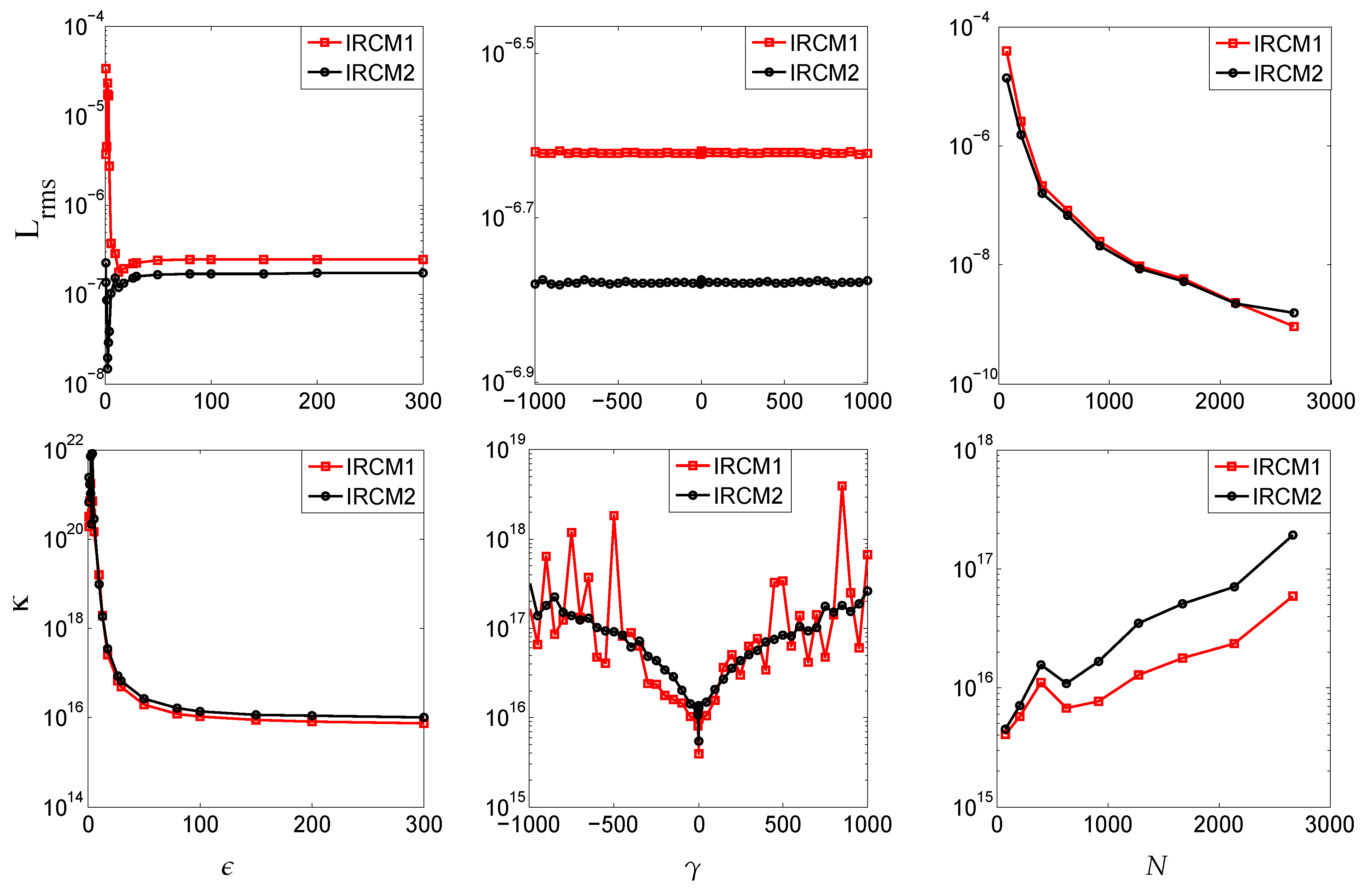
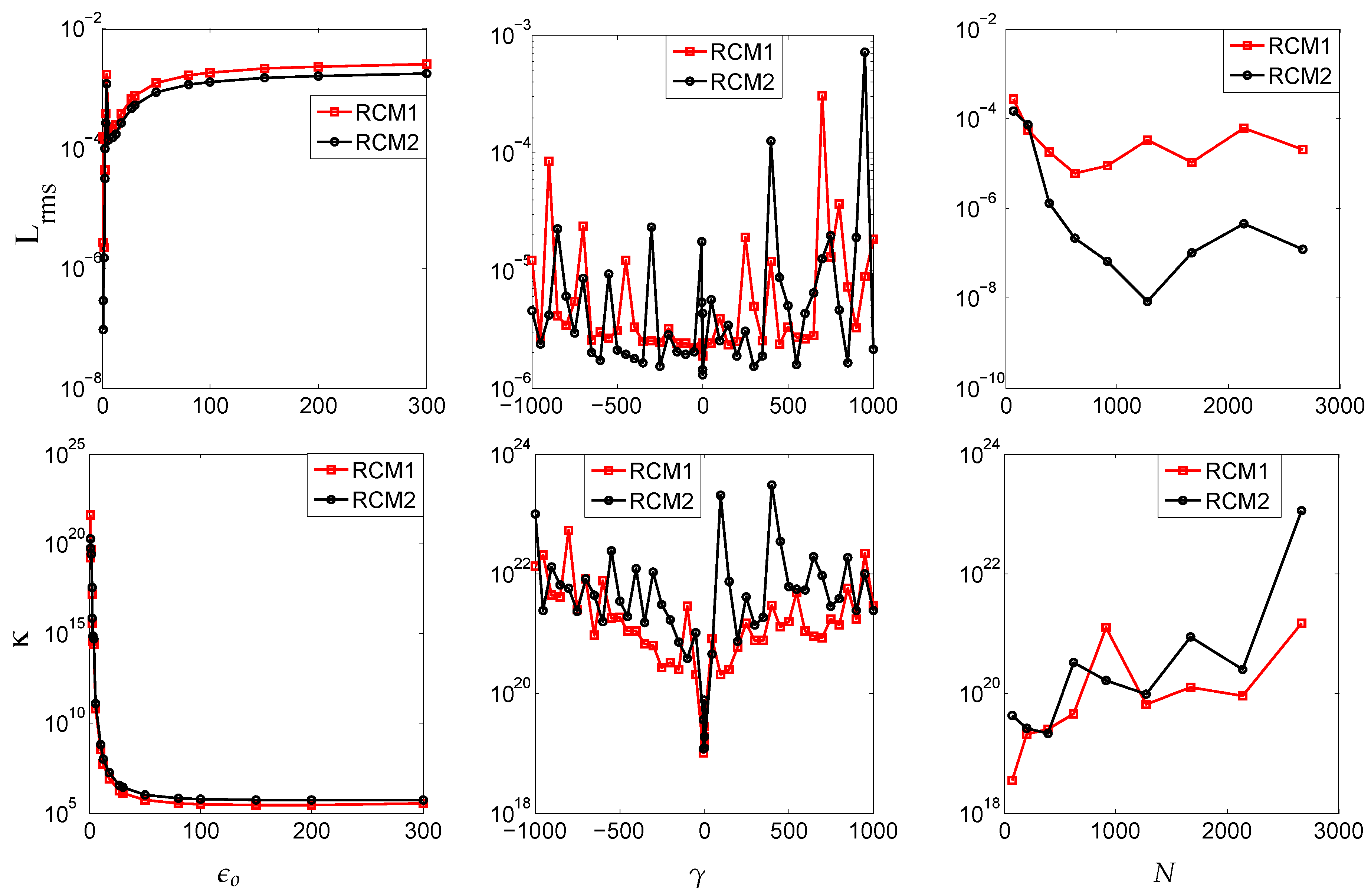
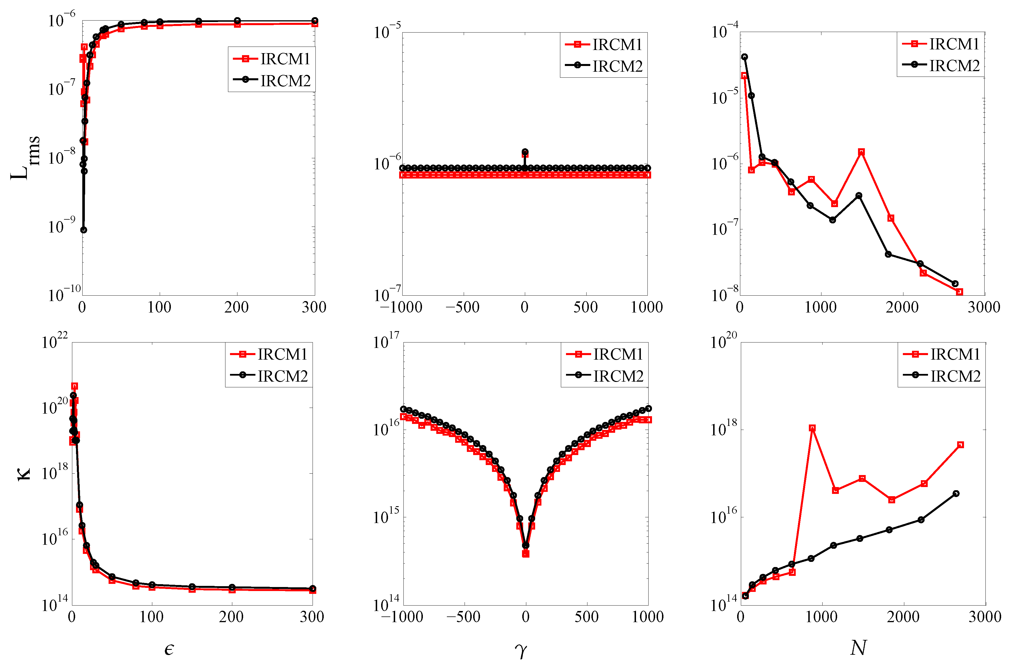
4. Numerical Experiments

In this section, the numerical results and the effect of nonlocal boundary condition (6) are demonstrated for (4). We discuss here different types of RBF-based collocation methods, i.e., RCM1, IRCM1, RCM2, and IRCM2. The effects of the shape parameters on the accuracy and $\kappa$ of the system matrices of the proposed methods are also investigated. This section shows that the proposed methods IRCM1 and IRCM2 are less sensitive to the selection of shape parameters as compared to RCM1 and RCM2.

Various error measures are used to estimate the accuracy of the numerical method. Among them, one is $L_{rms}$ error norm which is defined as

$$L_{rms}=\sqrt{\frac{1}{N}\sum _{i=1}^N{[\mathbf{u}\left(\widehat{\mathbf{v}}\right)-u\left(\widehat{\mathbf{v}}\right)]}^2},$$

(20)

where $\mathbf{u}\left(\widehat{\mathbf{v}}\right)$ and $u\left(\widehat{\mathbf{v}}\right)$ represent the exact and the approximate solutions respectively. One can also check the numerical stability of the method by $\kappa$ of the system matrix involved. A well conditioned system matrix has a small value of $\kappa$, while a system with larger value of $\kappa$ indicates that it is ill-conditioned. A built-in-function MATLAB command $cond(...)$ is used for this purpose. The benchmark problems having scattered interior points are taken from Halton set that utilizes the following MATLAB commands.

• R =$haltonset$(Dim), creates a Halton set on dimension Dim;
• O =$scramble$(R,’RR2’) gives a duplicate set, and RR2 is a scramble type;
• X =$net$(O,M) generates a $M\times Dim$ matrix containing the first M points in dimensions Dim from the point set O.

Problem 1.

The partial differential equation is given in (4) with constant coefficients $k_{1,1}\left(\widehat{v}\right)=-1$ and $k_{1,2}\left(\widehat{v}\right)=0$, and $k_{2,2}\left(\widehat{v}\right)=-1$ reduces to a Poisson equation and the one studied in reference [40] with the same nonlocal multipoint boundary condition. We consider the same problem with the same analytical solution

$$u\left(\widehat{v}\right)=xexp(y^2-1).$$

(21)

The domain is a unit rectangle having a cut of the radius $R=0.5$, which is depicted in Figure 1 (left). The functions f, g, and h are calculated according to the exact solution (21).

The representation of the solution domain and distribution of the nodes are depicted in Figure 1. In Figure 1 (right), the distinct scattered points marked with black dot represent an interior portion of the solution domain. The regularly distributed points marked with red dots represent the boundary parts ${\mathsf{\Gamma }}_2$, and the regularly distributed points marked with green dots represent the boundary parts ${\mathsf{\Gamma }}_1$. The scattered points marked with red asterisk are the points of the set ${\mathsf{\Omega }}^{★}$.

In case of Test Problem (1), the effects of the shape parameters ($ϵ$ or ${ϵ}_o$), the parameter $\gamma$, and the nodes are shown in Figure 2 and Figure 3 on the proposed methods using IMQ6 and MQ RBF as basis functions. From these figures, we can see that the methods based on IMQ6 RBF are better in accuracy and conditioning as compared to the methods based on MQ RBF. However, when the shape parameter is large, $\kappa$ of the methods based on MQ RBF is small but the accuracy of the methods is low. The methods RCM1 and RCM2 also give quite good results for some value of ${ϵ}_o$ (see Figure 3). The proposed methods IRCM1 and IRCM2 give reasonable accuracy for a wide range of $ϵ$ (see Figure 2). Figure 3 (right) shows that the RCM2 is more accurate than the RCM1 for dense grid and ${ϵ}_o=2$. However, $\kappa$ of RCM2 is worse than RCM1.

Figure 2 indicates that the IRCM1 is slightly better at conditioning than IRCM2. However, IRCM2 are much more accurate for a small value of $ϵ$. When the value of $ϵ$ increases, the error norms of the methods get closer to each other (see Figure 2 (left)). The conditioning performances of both methods IRCM1 and IRCM2 become better, up to certain limit when the value of $ϵ$ increases. After this limit, it does not much affect the $\kappa$ of the coefficient matrix. The behavior of IMQ6 RBF is the same as the MQ RBF, which gives quite good results for a small value of shape parameter along with high $\kappa$ of the coefficient matrix. Figure 2 (left) and Figure 3 (left) also indicate that accuracy of the IRCM1 and IRCM2 is better for a very wide range of the value of $ϵ$ as compared to the RCM1 and RCM2.

The effect of the collocation nodes on the accuracy of the proposed methods based on IMQ6 basis is also investigated. The value of the shape parameter is considered $ϵ=80$. The methods IRCM1 and IRCM2 give quite good results. As the nodal points increase, we see good agreement between solutions of IRCM1 and IRCM2 and the exact one. However, $\kappa$ increases for dense nodes while keeping the fixed value of the shape parameter $ϵ=80$.

The NBC (6) is defined comparatively on a small part of the boundary. However, from Figure 2 and Figure 3 (middle), we see that the NBC has a fairly strong negative influence on the $\kappa$ of the coefficient matrices corresponding to the methods RCM1, RCM2, IRCM1, and IRCM2. However, this influence is weak in case of IRCM1 and IRCM2 as compared to the methods RCM1 and RCM2. From Figure 2 (middle), we can observe that both the methods IRCM1 and IRCM2 give the same lowest and highest values of error norm. The highest and lowest error norms are $6.222\times {10}^{-7}$ and $6.184\times {10}^{-7}$ corresponding to $\gamma =2$ and $\gamma =0$. The influence of the NBC (6) is also weak on the $\kappa$ of the coefficient matrices corresponding to the methods IRCM1 and IRCM2 as compared to the methods RCM1 and RCM2. When ${ϵ}_o=2$ and $ϵ=80$, the methods RCM1 and RCM2 are the most ill-conditioned, and the absolute value of $\gamma$ increases as compared to the methods IRCM1 and IRCM2.

Problem 2.

Consider the equation given in (4) with variables coefficients $k_{1,1}\left(\widehat{v}\right)=5(1+x^2+y^2)$, $k_{1,2}\left(\widehat{v}\right)=1+\frac{xy}{2}$ and $k_{2,2}\left(\widehat{v}\right)=3(1+x^2+y^2)$. The functions f, g, and h are chosen such that the exact solution gets the form [59]:

$$u\left(\widehat{v}\right)=cos\left(y\right)exp(x-y).$$

Here in this example, we have considered an irregular-shaped domain defined by

$$x=p\left(\theta \right)cos\left(\theta \right),y=p\left(\theta \right)sin\left(\theta \right),p\left(\theta \right)=\frac{5-cos\left(4\theta \right)}{5},0\le \theta \le 2\pi ,$$

(22)

where $p\left(\theta \right)$ is the radius of the domain which depends on the polar angle θ.

The representation of the domain for Test Problem 2 is depicted in Figure 4. In Figure 4 (left), the boundary parts ${\mathsf{\Gamma }}_2$$(0\le \theta \le 2\pi /3)$ and ${\mathsf{\Gamma }}_1$$(2\pi /3<\theta <2\pi )$ are represented by red dashed and green solid lines respectively.

The influences of the shape parameters, the parameter $\gamma$, and nodal points on the accuracy and conditioning of the methods are shown in Figure 5 and Figure 6. The accuracy of IRCM2 is good as compared to the method IRCM1 for different values of shape parameter $ϵ$, as shown in Figure 5 (left). Both the methods are most poorly ill-conditioned for a small value of shape parameter $ϵ$, while the method IRCM2 gives high accuracy for a smaller value of $ϵ$ than IRMC1. It can be observed from these figures that the accuracy of the methods and $\kappa$ of the coefficient matrices for a fixed value of $ϵ$ increases when the number of nodes increases. In contrast to the methods based on MQ RBF, the $\kappa$ of the coefficient matrices of IRCM1 and IRCM2 is small. This is because of $ϵ$ which is large and is equal to 80. The system matrices of the proposed methods are ill-conditioned for a small value of $ϵ$. In addition, the effect of the parameter $\gamma$ on the methods IRCM1 and IRCM2 is also small. The method IRCM2 gives somewhat accurate results for all values of $\gamma$, even though the $\kappa$ of the coefficient matrix of IRCM1 is high for some values of $\gamma$ as compared to the method IRCM2 (see Figure 5 (middle)).

For dense nodes, RCM2 gives quite good results for ${ϵ}_o=2$ as compared to RCM1, as shown in Figure 6. However, the results obtained from IRCM1 and IRCM2 and the conditioning of the methods are much better there. Again in this example, the NBC (6) has a strong negative influence on the conditioning of the methods based on MQ RBF. From Figure 6, we see a fluctuation in $\kappa$ of the coefficient matrices associated with the methods RCM1 and RCM2 and in error norms as the value of $\gamma$ changes. This fluctuation in error norms occurs due to the small value of ${ϵ}_o$.

Problem 3.

Reconsider the differential equation given in (4) with constant coefficients $k_{1,1}\left(\widehat{v}\right)=3$, $k_{1,2}\left(\widehat{v}\right)=1.5$, and $k_{2,2}\left(\widehat{v}\right)=2$. The functions f, g, and h are chosen such that the exact solution gets the form [59]

$$u\left(\widehat{v}\right)=sin\left(\frac{x}{\sqrt{2}}\right)cosh\left(\frac{2\sqrt{30}}{15}x-\frac{\sqrt{30}}{10}y\right).$$

The representation of the domain for Test Problem 3 is depicted in Figure 7. The curve ${\mathsf{\Gamma }}_2\cup {\mathsf{\Gamma }}_1$ is called Cassini curve and is defined by parametric equation [59]:

$$x=\frac{4}{5}p\left(\theta \right)cos\left(\theta \right)-\frac{1}{5},y=\frac{4}{5}p\left(\theta \right)sin\left(\theta \right),p\left(\theta \right)={\left(cos\left(3\theta \right)+\sqrt{2-{sin}^2\left(3\theta \right)}\right)}^{1/3},0\le \theta \le 2\pi ,$$

(23)

and rest of the terms have the same meanings as defined in Test Problem 2. We consider the Neumann boundary condition on the boundary part ${\mathsf{\Gamma }}_1$. The normal component of the heat flux on the boundary is of the form:

$$-\left(k_{1,1}\left(\widehat{v}\right)\frac{\partial }{\partial x}u\left(\widehat{v}\right)+k_{1,2}\left(\widehat{v}\right)\frac{\partial }{\partial y}u\left(\widehat{v}\right)\right)n_x-\left(k_{1,2}\left(\widehat{v}\right)\frac{\partial }{\partial x}u+k_{2,2}\frac{\partial }{\partial y}u\left(\widehat{v}\right)\right)n_y=q\left(\widehat{v}\right),$$

(24)

where $q\left(\widehat{v}\right)$ is some given function. $n_x$ and $n_y$ are the components of unit outward normal vectors.

Since it was shown in the paper [59] that an RBF approximation of the mixed connected boundary conditions, i.e., Dirichlet boundary condition, is specified on some part of the boundary and Neumann condition, it is defined on the rest of boundary, and is too low in accuracy. If we specified Neumann boundary condition on boundary part ${\mathsf{\Gamma }}_1$, then the accuracy of the boundary condition would be too low. Since we used RBF approximation (i.e., using MQ or IMQ6 RBF) to approximate the mixed connected boundary condition, i.e., the multi-point and Neumann boundary condition, and the solution should be inside the domain. Hence, obviously, it would also affect the approximate solution inside the solution domain. To avoid this problem, we used the same procedure as was done above for the Dirichlet boundary condition but replaced the system of equation obtained from boundary part ${\mathsf{\Gamma }}_1$ with

$$\begin{array}{cc}\hfill -\sum _{k=1}^M{\beta }_k\{& \left(k_{1,1}\left(\widehat{v}\right)\frac{\partial }{\partial x}{\varphi }_k\left(\widehat{v}\right)+k_{1,2}\left(\widehat{v}\right)\frac{\partial }{\partial y}{\varphi }_k\left(\widehat{v}\right)\right)n_x+\left(k_{1,2}\left(\widehat{v}\right)\frac{\partial }{\partial x}{\varphi }_k+k_{2,2}\frac{\partial }{\partial y}{\varphi }_k\left(\widehat{v}\right)\right)n_y\}-\hfill \\ \hfill \sum _{i=1}^N{\lambda }_i\{& \left(k_{1,1}\left(\widehat{v}\right)\frac{\partial }{\partial x}({\varphi }_i\left(\widehat{v}\right)+{\omega }_i\left(\widehat{v}\right))+k_{1,2}\left(\widehat{v}\right)\frac{\partial }{\partial y}({\varphi }_i\left(\widehat{v}\right)+{\omega }_i\left(\widehat{v}\right))\right)n_x+\hfill \\ \hfill & \left(k_{1,2}\left(\widehat{v}\right)\frac{\partial }{\partial x}({\varphi }_i\left(\widehat{v}\right)+{\omega }_i\left(\widehat{v}\right))+k_{2,2}\frac{\partial }{\partial y}({\varphi }_i\left(\widehat{v}\right)+{\omega }_i\left(\widehat{v}\right))\right)n_y\}=q\left(\widehat{v}\right),\widehat{v}\in {\widehat{\mathsf{\Gamma }}}_1.\hfill \end{array}$$

(25)

The influences of shape parameters ($ϵ$ or ${ϵ}_o$), the parameter $\gamma$, and the number of nodes for Test problem 3 are shown in Figure 8 and Figure 9. It can be seen from Figure 8 and Figure 9 (right) that the proposed methods give good accuracy for dense grid whether the RBF basis is MQ or IMQ6. However, the $\kappa$ of the coefficient matrices associated with the methods RCM1 and RCM2 are high. From Figure 8 (top middle), we see that when $\gamma =0$ the error norms of the methods IRCM1 and IRCM2 are $1.175\times {10}^{-6}$ and $1.226\times {10}^{-6}$ respectively.

Now we check the influence of the parameter $\gamma$ on the methods IRCM1 and IRCM2 when the shape parameter is small. The value of the shape parameter $ϵ=2$ is taken for each problem. We see from Figure 10 that IRCM2 give quite a good accuracy for a small value of shape parameter in all Test Problems 1–3. The accuracy is good when the value of $\gamma$ is zero or near to zero. It can be observed from this figure that the $\kappa$ and the accuracies of the proposed methods deteriorate when the absolute value of $\gamma$ increases. In contrast, when the value of shape parameter is high (i.e., $ϵ=80$) the $\kappa$ deteriorates but the accuracy does not affect much when $\left|\gamma \right|$ is increased (see middle of Figure 2, Figure 5 and Figure 8). The absolute error of IRCM1 and IRCM2 of the unknown solution on the boundary part ${\mathsf{\Gamma }}_2$ is shown in Figure 11. From this figure, we observed that both the methods IRCM1 and IRCM2 give quite good accuracy.

Accuracy in terms of error norm and conditioning of the coefficient matrices corresponding to the proposed methods is shown in Figure 12. The values of the parameters are $ϵ=150$, ${ϵ}_o=2$, and $\gamma =20$. We observed from this figure that the proposed methods based on integrated MQ RBF performed well both in terms of accuracy and conditioning. We have also seen that different types of boundary conditions (i.e., Dirichlet and Neumann conditions) do not much affect the conditioning and accuracy of the proposed methods IRCM1 and IRCM2.

5. Conclusions

The collocation methods based on MQ and IMQ6 were set up for the numerical solution of elliptic NMBC with variable coefficients. The results of the propsed extended methods were compared with Kansa’s approach. The method based on IMQ6 RBF is well conditioned as compared to the collocation method based on MQ RBF (see Figure 11) for a large value of the shape parameter $ϵ$. However, the methods IRCM1, IRCM2, RCM1, and RCM2 became ill-conditioned for small values of shape parameter $ϵ$ (see Figure 2, Figure 3, Figure 5, Figure 6, Figure 8, and Figure 9) but the results are reasonably accurate. This approach can be extended to a higher dimension easily. In addition, the proposed approach can be applied to time-dependent PDEs with nonlocal multi-point boundary conditions.

References

1. Chen, C.K.; Fife, P. Nonlocal models of phase transitions in solids. Adv. Math. Sci. Appl. 2000, 10, 821–849. [Google Scholar]
2. Lacey, A. Thermal runaway in a non-local problem modelling ohmic heating. part ii: General proof of blow-up and asymptotics of runaway. Eur. J. Appl. Math. 1995, 6, 201–224. [Google Scholar] [CrossRef]
3. Bebernes, J.; Talaga, P. Nonlocal problems modelling shear banding. Commun. Appl. Nonlinear Anal. 1996, 3, 79–103. [Google Scholar]
4. Bebernes, J.; Li, C.; Talaga, P. Single-point blowup for nonlocal parabolic problems. Phys. D Nonlinear Phenom. 1999, 134, 48–60. [Google Scholar] [CrossRef]
5. Lacey, A. Mathematical analysis of thermal runaway for spatially inhomogeneous reactions. SIAM J. Appl. Math. 1983, 43, 1350–1366. [Google Scholar] [CrossRef]
6. Caglioti, E.; Lions, P.L.; Marchioro, C.; Pulvirenti, M. A special class of stationary flows for two-dimensional euler equations: A statistical mechanics description. Commun. Math. Phys. 1992, 143, 501–525. [Google Scholar] [CrossRef]
7. Furter, J.; Grinfeld, M. Local vs. non-local interactions in population dynamics. J. Math. Biol. 1989, 27, 65–80. [Google Scholar] [CrossRef]
8. Wolansky, G. A critical parabolic estimate and application to nonlocal equations arising in chemotaxis. Appl. Anal. 1997, 66, 291–321. [Google Scholar] [CrossRef]
9. Gilboa, G.; Osher, S. Nonlocal operators with applications to image processing. Multiscale Model. Simul. 2009, 7, 1005–1028. [Google Scholar] [CrossRef]
10. Dehghan, M. Efficient techniques for the second-order parabolic equation subject to nonlocal specifications. Appl. Numer. Math. 2005, 52, 39–62. [Google Scholar] [CrossRef]
11. Aziz, I.; Ahmad, M. Numerical solution of two-dimensional elliptic PDEs with nonlocal boundary conditions. Comput. Math. Appl. 2015, 69, 180–205. [Google Scholar] [CrossRef]
12. Ma, R. A survey on nonlocal boundary value problems. Appl. Math. E-Notes 2007, 7, 257–279. [Google Scholar]
13. Eziani, D.G.; Shvili, G.A. Investigation of the nonlocal initial boundary value problems for some hyperbolic equations. Hiroshima Math. J. 2001, 31, 345–366. [Google Scholar]
14. Berikelashvili, G.; Khomeriki, N. On a numerical solution of one nonlocal boundary-value problem with mixed dirichlet–neumann conditions. Lith. Math. J. 2013, 53, 367–380. [Google Scholar] [CrossRef]
15. Mollapourasl, R. An efficient numerical scheme for a nonlinear integro-differential equations with an integral boundary condition. Appl. Math. Comput. 2014, 248, 8–17. [Google Scholar] [CrossRef]
16. Fasshauer, G. Meshfree Approximation Methods With Matlab; World Scientific Publishing Co. Pte. Ltd.: Singapore, 2007; Volume 6. [Google Scholar]
17. Sarra, S. Integrated multiquadric radial basis function approximation methods. Comput. Math. Appl. 2006, 51, 1283–1296. [Google Scholar] [CrossRef] [Green Version]
18. Hardy, R. Multiquadratic equations for topography and other irregular surfaces. J. Geophys. Res. 1971, 76, 1905–1915. [Google Scholar] [CrossRef]
19. Franke, R. Scattered data interpolation tests of some methods. Math. Comput. 1982, 38, 181–200. [Google Scholar] [CrossRef]
20. Fasshauer, G. Newton iteration with multiquadratics for the solution of nonlinear PDEs. Comput. Math. Appl. 2002, 43, 423–438. [Google Scholar] [CrossRef] [Green Version]
21. Wang, J.; Liu, G. On the optimal shape parameters of radial basis functions used for 2-D meshless methods. Comput. Methods Appl. Mech. Eng. 2002, 191, 2611–2630. [Google Scholar] [CrossRef]
22. Ballestra, L.; Pacelli, G. Computing the survival probability density function in jump-diffusion models: A new approach based on radial basis functions. Eng. Anal. Bound. Elem. 2011, 35, 1075–1084. [Google Scholar] [CrossRef]
23. Ballestra, L.; Pacelli, G. Pricing European and American options with two stochastic factors: A highly efficient radial basis function approach. J. Econ. Dyn. Control 2013, 37, 1142–1167. [Google Scholar] [CrossRef]
24. Luh, L. The shape parameter in the Gaussian function. Comput. Math. Appl. 2012, 63, 453–461. [Google Scholar] [CrossRef] [Green Version]
25. Davydov, O.; Oanh, D. On the optimal shape parameter for Gaussian radial basis function finite difference approximation of the Poisson equation. Comput. Math. Appl. 2001, 62, 27–49. [Google Scholar] [CrossRef] [Green Version]
26. Cheng, A. Multiquadric and its shape parameter—A numerical investigation of error estimate, condition number, and round-off error by arbitrary precision computation. Eng. Anal. Bound. Elem. 2012, 36, 220–239. [Google Scholar] [CrossRef]
27. Huang, C.; Yen, H.; Cheng, A. On the increasingly flat radial basis function and optimal shape parameter for the solution of elliptic PDEs. Eng. Anal. Bound. Elem. 2010, 34, 802–809. [Google Scholar] [CrossRef]
28. Scheuerer, M. An alternative procedure for selecting a good value for the parameter c in RBF-interpolation. Adv. Comput. Math. 2011, 34, 105–126. [Google Scholar] [CrossRef] [Green Version]
29. Uddin, M. On the selection of a good value of shape parameter in solving time-dependent partial differential equations using RBF approximation method. Appl. Math. Model. 2014, 38, 135–144. [Google Scholar] [CrossRef]
30. Esmaeilbeigi, M.; Hosseini, M. A new approach based on the genetic algorithm for finding a good shape parameter in solving partial differential equations by Kansa’s method. Appl. Math. Comput. 2014, 249, 419–428. [Google Scholar] [CrossRef]
31. Kazem, S.; Hadinejad, F. Promethee technique to select the best radial basis functions for solving the 2-dimensional heat equations based on hermite interpolation. Eng. Anal. Bound. Elem. 2015, 50, 29–38. [Google Scholar] [CrossRef]
32. Golbabi, A.; Mohebianfar, E.; Rabiei, H. On the new variable shape parameter strategies for radial basis functions. Comput. Appl. Math. 2015, 34, 691–704. [Google Scholar] [CrossRef]
33. Kadalbajoo, M.; Kumar, A.; Tripathi, L. A radial basis functions based finite differences method for wave equation with an integral condition. Appl. Math. Comput. 2015, 238, 8–16. [Google Scholar] [CrossRef]
34. Yan, L.; Yang, F. The method of approximate particular solutions for the time-fractional diffusion equation with non-local boundary condition. Comput. Math. Appl. 2015, 70, 2716–2732. [Google Scholar] [CrossRef]
35. Dehghan, M.; Tatari, M. On the solution of the non-local parabolic partial differential equations via radial basis functions. Appl. Math. Model. 2009, 52, 461–477. [Google Scholar]
36. Dehghan, M.; Shokri, A. A meshless method for numerical solution of the one-dimensional wave equation with an integral conditions using radial basis functions. Numer. Algorithms 2009, 52, 461–477. [Google Scholar] [CrossRef]
37. Kazem, S.; Rad, J. Radial basis functions method for solving of a non-local boundary value problem with neumann’s boundary conditions. Appl. Math. Model. 2012, 36, 2360–2369. [Google Scholar] [CrossRef]
38. Sajavicius, S. Optimization, conditioning and accuracy of radial basis function method for partial differential equations with nonlocal boundary conditions—A case of two-dimensional poisson equation. Eng. Anal. Bound. Elem. 2013, 37, 788–804. [Google Scholar] [CrossRef]
39. Sajavicius, S. Radial basis function method for a multidimensional linear elliptic equation with nonlocal boundary conditions. Comput. Math. Appl. 2014, 87, 1407–1420. [Google Scholar] [CrossRef]
40. Sajavicius, S. Radial basis function collocation method for an elliptic problem with nonlocal multipoint boundary condition. Eng. Anal. Bound. Elem. 2016, 67, 164–172. [Google Scholar] [CrossRef]
41. Siraj-ul-Islm; Ahmad, M. Meshless analysis of elliptic interface boundary value problems. Eng. Anal. Bound. Elem. 2018, 92, 38–49. [Google Scholar] [CrossRef]
42. Ahmad, M.; Siraj-ul-Islm. Meshless analysis of parabolic interface problems. Eng. Anal. Bound. Elem. 2018, 94, 134–152. [Google Scholar]
43. Ahmad, M.; Siraj-ul-Islm; Larsson, E. Local meshless methods for second order elliptic interface problems with sharp corners. J. Comput. Phys. 2020, 416, 109500. [Google Scholar]
44. Zaheer-ud-Din; Siraj-ul-Islam; Mati ur Rahman. Oscillatory discontinuous kernel based meshless technique of Fredholm integral equation. In Proceedings of the International Conference on Applied and Engineering Mathematics (ICAEM), Taxila, Pakistan, 4–5 September 2018; pp. 53–55. [Google Scholar]
45. Zaheer-ud-Din; Siraj-ul-Islam. RBF Solution Method for 1D Oscillatory Fredholm Integral Equations Having Kernel Function Free-of-Stationary-Points. In Proceedings of the 14th Regional Conference on Mathematical Physics, Islamabad, Pakistan, 9–14 November 2015; World Scientific Publishing Co. Pte. Ltd.: Singapore, 2017; pp. 284–292. [Google Scholar]
46. Zaheer-ud-Din; Siraj-ul-Islam. Kernel-based meshless approximation of one-dimensional oscillatory Fredholm integral equations. FILOMAT 2020, 34, 3:5743–5753. [Google Scholar]
47. Siraj-ul-Islam; Aziz, I.; Zaheer-ud-Din. Meshless methods for multivariate highly oscillatory Fredholm integral equations. Eng. Anal. Bound. Elem. 2015, 53, 100–112. [Google Scholar]
48. Zaheer-ud-Din; Siraj-ul-Islam. Meshless methods for one-dimensional oscillatory Fredholm integral equations. Appl. Math. Comput. 2018, 324, 156–173. [Google Scholar]
49. Siraj-ul-Islam; Zaheer-ud-Din. Meshless methods for two-dimensional oscillatory Fredholm integral equations. J. Comput. Appl. Math. 2018, 335, 33–50. [Google Scholar] [CrossRef]
50. Ahmad, M.; Siraj-ul-Islam; Ullah, B. Local radial basis function collocation method for stokes equations with interface conditions. Eng. Anal. Bound. Elem. 2020, 119, 246–256. [Google Scholar]
51. Ahmad, I.; Ahsan, M.; Zaheer-ud-Din; Masood, A.; Kumam, P. An efficient local formulation for time–dependent PDEs. Mathematics 2019, 7, 216. [Google Scholar]
52. Ling, L.; Trummer, M. Multiquadric collocation method with integral formulation for boundary layer problems. Comput. Math. Appl. 2004, 48, 927–941. [Google Scholar]
53. Mai-Duy, N.; Tran-Cong, T. A multidomain integrated radial basis function collocation method for elliptic problems. Appl. Math. Model. 2003, 27, 197–220. [Google Scholar]
54. Mai-Duy, N.; Tran-Cong, T. Solving high order ordinary differential equations with radial basis function networks. Int. J. Numer. Methods Eng. 2005, 62, 824–852. [Google Scholar] [CrossRef] [Green Version]
55. Mai-Duy, N.; Tran-Cong, T. Solving high order partial differential equations with indirect radial basis function networks. Int. J. Numer. Methods Eng. 2006, 63, 1636–1654. [Google Scholar] [CrossRef] [Green Version]
56. Kansa, E.; Power, H.; Fasshauer, G.; Ling, L. A volumetric integral radial basis function method for time-dependent partial differential equation: I. formulation. Eng. Anal. Bound. Elem. 2004, 28, 1191–1206. [Google Scholar] [CrossRef]
57. Mai-Duy, N.; Tran-Cong, T. An integrated-RBF technique based on Garlerkin formulation for elliptic differential equations. Eng. Anal. Bound. Elem. 2009, 33, 191–199. [Google Scholar]
58. Thai-Quang, N.; Le-Cao, K.; Mai-Duy, N.; Tran, C.; Tran-Cong, T. A numerical scheme based on compact integrated RBFs and Adams- Bashforth/Crank–Nicolson algorithms for diffusion and unsteady fluid flow problems. Eng. Anal. Bound. Elem. 2013, 37, 1653–1667. [Google Scholar] [CrossRef]
59. Reutskiy, S. A meshless radial basis function method for 2D steady-state heat conduction problems in anisotropic and inhomogeneous media. Eng. Anal. Bound. Elem. 2016, 66, 1–11. [Google Scholar] [CrossRef]
Figure 1. Model domain for Test Problem (1).
Mathematics 08 02045 g001
Figure 2. Test Problem 1, accuracy and κ versus ϵ , γ m, and N: Γ ^ 1 = 60 , Γ ^ 2 = 16 , γ = 1 , ϵ = 80 , and N = 94 when its influence is interestless.
Mathematics 08 02045 g002
Figure 3. Test Problem 1, accuracy and κ versus ϵ o , γ , and N: Γ ^ 1 = 60 , Γ ^ 2 = 16 , γ = 1 , ϵ o = 2 , and N = 94 when its influence is interestless.
Mathematics 08 02045 g003
Figure 4. Model domain for test problem 2.
Mathematics 08 02045 g004
Figure 5. Test Problem 2, accuracy and κ versus ϵ , γ , and N: Γ ^ 1 = 94 , Γ ^ 2 = 46 , γ = 1 , ϵ = 80 , and N = 320 when its influence is interestless.
Mathematics 08 02045 g005
Figure 6. Test Problem 2, accuracy and κ versus ϵ o , γ , and N: Γ ^ 1 = 94 , Γ ^ 2 = 46 , γ = 1 , ϵ o = 2 , and N = 320 when its influence is interestless.
Mathematics 08 02045 g006
Figure 7. Model domain for Test Problem 3.
Mathematics 08 02045 g007
Figure 8. Test Problem 3, accuracy and κ versus ϵ , γ and N: Γ ^ 1 = 67 , Γ ^ 2 = 33 , γ = 1 , ϵ o = 2 , ϵ = 80 , and N = 312 when its influence is interestless.
Mathematics 08 02045 g008
Figure 9. Test Problem 3, accuracy and κ versus ϵ o , γ and N: Γ ^ 1 = 67 , Γ ^ 2 = 33 , γ = 1 , ϵ o = 2 , and N = 312 when its influence is interestless.
Mathematics 08 02045 g009
Figure 10. Test Problems 1–3, accuracy and κ versus γ and ϵ = 2 .
Mathematics 08 02045 g010
Figure 11. Test Problems 1–3, absolute errors | u ( v ^ ) u ( v ^ ) | using the methods IRCM1 and IRCM2 versus x on boundary parts Γ 2 , ϵ = 80 , and γ = 1 .
Mathematics 08 02045 g011
Figure 12. Test Problems 1–3, accuracy and κ versus N. ϵ = 150 , ϵ o = 2 , and γ = 20 .
Mathematics 08 02045 g012
Publisher’s Note: MDPI stays neutral with regard to jurisdictional claims in published maps and institutional affiliations.