Principle of Duality in Cubic Smoothing Spline

Abstract

Fitting a cubic smoothing spline is a typical smoothing method. This paper reveals a principle of duality in the penalized least squares regressions relating to the method. We also provide a number of results derived from them, some of which are illustrated by a real data example.

1. Introduction

Fitting a cubic smoothing spline, which was developed by [1,2] and others, is a typical smoothing method. The cubic smoothing spline fitted to a scatter plot of ordered pairs $(x_i,y_i)$ for $i=1,\dots ,n$ is a function such that

$$\begin{array}{c}\hfill \widehat{f}\left(x\right)=\arg \underset{f\in \mathcal{W}}{min}\sum _{i=1}^n{\left\{y_i-f\left(x_i\right)\right\}}^2+\lambda {\int }_a^b{\left\{f^{″}\left(x\right)\right\}}^{2}dx,\end{array}$$

(1)

where $x_1,\dots ,x_n$ are points satisfying $a<x_1<\cdots <x_n<b$, $\mathcal{W}$ denotes a function space that contains all functions of which the second derivative is square integrable over $[a,b]$, and $\lambda$ is a positive smoothing/tuning parameter, which controls the trade-off between goodness of fit and smoothness.

Let $\widehat{\mathit{f}}={[\widehat{f}\left(x_1\right),\dots ,\widehat{f}\left(x_n\right)]}^{\top }$. Then, given $\widehat{f}\left(x\right)$ is a natural cubic spline of which the knots are $x_1,\dots ,x_n$ (see, e.g., [3,4]), it follows that

$$\begin{array}{cc}\hfill \widehat{\mathit{f}}& =\arg \underset{\mathit{f}\in {\mathbb{R}}^n}{\min }{\parallel \mathit{y}-\mathit{f}\parallel }^2+\lambda {\mathit{f}}^{\top }{\mathit{C}}^{\top }{\mathit{R}}^{-1}\mathit{C}\mathit{f}\hfill \end{array}$$

(2)

$$\begin{array}{cc}\hfill & ={\left({\mathit{I}}_n+\lambda {\mathit{C}}^{\top }{\mathit{R}}^{-1}\mathit{C}\right)}^{-1}\mathit{y},\hfill \end{array}$$

(3)

where $\mathit{y}={[y_1,\dots ,y_n]}^{\top }$, ${\mathit{I}}_n$ denotes the $n\times n$ identity matrix, and $\mathit{C}$ and $\mathit{R}$ are explicitly presented later. Then, as shown in [3], $\widehat{f}\left(x\right)$ in (1) is uniquely determined by $\widehat{\mathit{f}}\in {\mathbb{R}}^n$ in (3). Thus, estimating $\widehat{f}\left(x\right)$ is equivalent to estimating $\widehat{\mathit{f}}$.

Let $\mathsf{\Pi }=[{\mathbf{\iota }}_n,\mathit{x}]\in {\mathbb{R}}^{n\times 2}$, where ${\mathbf{\iota }}_n={[1,\dots ,1]}^{\top }\in {\mathbb{R}}^n$ and $\mathit{x}={[x_1,\dots ,x_n]}^{\top }$. Note that since $x_1<\cdots <x_n$, ${\mathbf{\iota }}_n$ and $\mathit{x}$ are linearly independent and thus $\mathsf{\Pi }$ is of full column rank. Let

$$\begin{array}{c}\hfill \widehat{\mathbf{\tau }}=\mathsf{\Pi }{\left({\mathsf{\Pi }}^{\top }\mathsf{\Pi }\right)}^{-1}{\mathsf{\Pi }}^{\top }\mathit{y}.\end{array}$$

(4)

Denote the difference between $\widehat{\mathit{f}}$ and $\widehat{\mathbf{\tau }}$ (resp. $\mathit{y}$ and $\widehat{\mathit{f}}$) by $\widehat{\mathit{c}}$ (resp. $\widehat{\mathit{u}}$):

$$\begin{array}{c}\hfill \widehat{\mathit{c}}=\widehat{\mathit{f}}-\widehat{\mathbf{\tau }},\widehat{\mathit{u}}=\mathit{y}-\widehat{\mathit{f}}.\end{array}$$

(5)

Accordingly, we have

$$\begin{array}{c}\hfill \mathit{y}=\widehat{\mathbf{\tau }}+\widehat{\mathit{c}}+\widehat{\mathit{u}}.\end{array}$$

(6)

In this paper, we present a comprehensive list of penalized least squares regressions relating to (6). One such example is the ridge regression [5] that leads to $\widehat{\mathit{c}}$. Then, we reveal a principle of duality in them. In addition, based on them, we provide a number of theoretical results, for example, ${\mathbf{\iota }}_n^{\top }\widehat{\mathit{c}}=0$.

This paper is organized as follows. Section 2 fixes some notations and gives key preliminary results used to derive the main results in the paper. Section 3 provides a comprehensive list of penalized least squares regressions relating to (6), and reveals a principle of duality in them. Section 4 shows some results that are obtainable from the regressions shown in Section 3. Section 5 illustrates some results provided in Section 3 and Section 4 by a real data example. Section 6 deals with the cases such that the other right-inverse matrices are used. Section 7 concludes the paper.

2. Preliminaries

In this section, we give key preliminary results used to derive the main results of this paper. Before stating them, we fix some notations.

2.1. Notations

Let ${\widehat{f}}_i$ (resp. ${\widehat{\tau }}_i$) denote the ith entry of $\widehat{\mathit{f}}$ (resp. $\widehat{\mathbf{\tau }}$) for $i=1,\dots ,n$, ${\delta }_i=x_{i+1}-x_i$, which is positive by definition, for $i=1,\dots ,n-1$, $\mathsf{\Delta }=\mathsf{diag}({\delta }_1,\dots ,{\delta }_{n-1})\in {\mathbb{R}}^{(n-1)\times (n-1)}$, and for a full-row-rank matrix $\mathit{M}\in {\mathbb{R}}^{m\times n}$, ${\mathit{M}}^{\top }{\left(\mathit{M}{\mathit{M}}^{\top }\right)}^{-1}\in {\mathbb{R}}^{n\times m}$, which is a right-inverse matrix of $\mathit{M}$, be denoted by ${\mathit{M}}_{\mathrm{r}}^{-1}$. For a full-column-rank matrix $\mathit{W}\in {\mathbb{R}}^{n\times p}$, let $\mathcal{S}\left(\mathit{W}\right)$ (resp. ${\mathcal{S}}^{\perp }\left(\mathit{W}\right)$) denote the column space of $\mathit{W}$ (resp. the orthogonal complement of $\mathcal{S}\left(\mathit{W}\right)$) and ${\mathit{P}}_W$ (resp. ${\mathit{Q}}_W$) denote the orthogonal projection matrix to the space $\mathcal{S}\left(\mathit{W}\right)$ (resp. ${\mathcal{S}}^{\perp }\left(\mathit{W}\right)$). Explicitly, they are ${\mathit{P}}_W=\mathit{W}{\left({\mathit{W}}^{\top }\mathit{W}\right)}^{-1}{\mathit{W}}^{\top }$ and ${\mathit{Q}}_W={\mathit{I}}_n-{\mathit{P}}_W$. ${\mathit{D}}_{\left(i\right)}\in {\mathbb{R}}^{(n-i)\times (n-i+1)}$ is a Toeplitz matrix of which the first (resp. last) row is $[-1,1,0,\dots ,0]$ (resp. $[0,\dots ,0,-1,1]$) and we define matrices $\mathit{C}\in {\mathbb{R}}^{(n-2)\times n}$ and $\mathit{R}\in {\mathbb{R}}^{(n-2)\times (n-2)}$ as follows:

$$\begin{array}{c}\hfill \mathit{C}=\left[\begin{array}{cccccc}{\delta }_1^{-1}& -{\delta }_1^{-1}-{\delta }_2^{-1}& {\delta }_2^{-1}& 0& \cdots & 0\\ 0& \ddots & \ddots & \ddots & \ddots & ⋮\\ ⋮& \ddots & \ddots & \ddots & \ddots & 0\\ 0& \cdots & 0& {\delta }_{n-2}^{-1}& -{\delta }_{n-2}^{-1}-{\delta }_{n-1}^{-1}& {\delta }_{n-1}^{-1}\end{array}\right]\end{array}$$

(7)

and

$$\begin{array}{c}\hfill \mathit{R}=\left[\begin{array}{ccccc}\frac{1}{3}({\delta }_1+{\delta }_2)& \frac{1}{6}{\delta }_2& 0& \cdots & 0\\ \frac{1}{6}{\delta }_2& \frac{1}{3}({\delta }_2+{\delta }_3)& \ddots & \ddots & ⋮\\ 0& \ddots & \ddots & \ddots & 0\\ ⋮& \ddots & \ddots & \ddots & \frac{1}{6}{\delta }_{n-2}\\ 0& \cdots & 0& \frac{1}{6}{\delta }_{n-2}& \frac{1}{3}({\delta }_{n-2}+{\delta }_{n-1})\end{array}\right].\end{array}$$

(8)

Finally, we denote the eigenvalues of $\mathit{R}$ by ${\omega }_1,\dots ,{\omega }_{n-2}$ in descending order.

2.2. Key Preliminary Results

Lemma 1.

(i) 

$\mathit{C}$ can be factorized as $\mathit{C}={\mathit{D}}_{\left(2\right)}{\mathsf{\Delta }}^{-1}{\mathit{D}}_{\left(1\right)}$.

(ii) 

We have the following inequalities:

$$\begin{array}{c}\hfill {\omega }_{n-2}\ge min\left\{\frac{1}{3}{\delta }_1+\frac{1}{6}{\delta }_2,\frac{1}{6}({\delta }_2+{\delta }_3),\dots ,\frac{1}{6}({\delta }_{n-3}+{\delta }_{n-2}),\frac{1}{6}{\delta }_{n-2}+\frac{1}{3}{\delta }_{n-1}\right\}>0.\end{array}$$

Proof of Lemma 1.

(i)

Let $\mathit{w}={[w_1,\dots ,w_n]}^{\top }$ be an n-dimensional column vector. Then, by definition of $\mathit{C}$, it follows that

$$\begin{array}{cc}\hfill \mathit{C}\mathit{w}& =\left[\begin{array}{c}-\frac{w_2-w_1}{{\delta }_1}+\frac{w_3-w_2}{{\delta }_2}\\ ⋮\\ -\frac{w_{n-1}-w_{n-2}}{{\delta }_{n-2}}+\frac{w_n-w_{n-1}}{{\delta }_{n-1}}\end{array}\right]={\mathit{D}}_{\left(2\right)}\left[\begin{array}{c}\frac{w_2-w_1}{{\delta }_1}\\ ⋮\\ \frac{w_n-w_{n-1}}{{\delta }_{n-1}}\end{array}\right]={\mathit{D}}_{\left(2\right)}{\mathsf{\Delta }}^{-1}\left[\begin{array}{c}-w_1+w_2\\ ⋮\\ -w_{n-1}+w_n\end{array}\right]\hfill \\ \hfill & ={\mathit{D}}_{\left(2\right)}{\mathsf{\Delta }}^{-1}{\mathit{D}}_{\left(1\right)}\mathit{w}\in {\mathbb{R}}^{n-2},\hfill \end{array}$$

which leads to $\mathit{C}={\mathit{D}}_{\left(2\right)}{\mathsf{\Delta }}^{-1}{\mathit{D}}_{\left(1\right)}$.

(ii)

The first inequality follows by applying the Gershgorin circle theorem and the second inequality holds from ${\delta }_i>0$ for $i=1,\dots ,n-1$.

 □

Remark 1.

In Appendix A, we give some remarks on a special case such that $\mathit{x}={[1,\dots ,n]}^{\top }$.

Lemma 2.

(i) 

$\mathcal{S}\left({\mathit{C}}^{\top }\right)$ equals ${\mathcal{S}}^{\perp }\left(\mathsf{\Pi }\right)$ and

(ii) 

$\mathcal{S}\left({\mathit{C}}_{\mathrm{r}}^{-1}\right)$ equals ${\mathcal{S}}^{\perp }\left(\mathsf{\Pi }\right)$.

Proof of Lemma 2.

(i)

Given that ${\delta }_i>0$ for $i=1,\dots ,n-1$, both $\mathsf{\Pi }$ and ${\mathit{C}}^{\top }$ are of full column rank. In addition, $[\mathsf{\Pi },{\mathit{C}}^{\top }]$ is a square matrix. Thus, if ${\left({\mathit{C}}^{\top }\right)}^{\top }\mathsf{\Pi }=\mathit{C}\mathsf{\Pi }=\mathbf{0}$, then it follows that $\mathcal{S}\left({\mathit{C}}^{\top }\right)={\mathcal{S}}^{\perp }\left(\mathsf{\Pi }\right)$. From ${\mathit{D}}_{\left(1\right)}{\mathbf{\iota }}_n=\mathbf{0}$, we have $\mathit{C}{\mathbf{\iota }}_n={\mathit{D}}_{\left(2\right)}{\mathsf{\Delta }}^{-1}{\mathit{D}}_{\left(1\right)}{\mathbf{\iota }}_n=\mathbf{0}$. Likewise, from ${\mathsf{\Delta }}^{-1}{\mathit{D}}_{\left(1\right)}\mathit{x}={\mathsf{\Delta }}^{-1}\mathsf{\Delta }{\mathbf{\iota }}_{n-1}={\mathbf{\iota }}_{n-1}$ and ${\mathit{D}}_{\left(2\right)}{\mathbf{\iota }}_{n-1}=\mathbf{0}$, we obtain $\mathit{C}\mathit{x}={\mathit{D}}_{\left(2\right)}{\mathsf{\Delta }}^{-1}{\mathit{D}}_{\left(1\right)}\mathit{x}=\mathbf{0}$. Accordingly, we have $\mathit{C}\mathsf{\Pi }=\mathbf{0}$, which completes the proof.

(ii)

Recall that ${\mathit{C}}_{\mathrm{r}}^{-1}={\mathit{C}}^{\top }{\left(\mathit{C}{\mathit{C}}^{\top }\right)}^{-1}$. It is clear that ${\mathit{C}}_{\mathrm{r}}^{-1}$ is a full-column-rank matrix such that $[\mathsf{\Pi },{\mathit{C}}_{\mathrm{r}}^{-1}]$ is a square matrix. In addition, ${\left({\mathit{C}}_{\mathrm{r}}^{-1}\right)}^{\top }\mathsf{\Pi }={\left(\mathit{C}{\mathit{C}}^{\top }\right)}^{-1}\mathit{C}\mathsf{\Pi }=\mathbf{0}$. Thus, it follows that $\mathcal{S}\left({\mathit{C}}_{\mathrm{r}}^{-1}\right)={\mathcal{S}}^{\perp }\left(\mathsf{\Pi }\right)$.

 □

Denote the spectral decomposition of $\mathit{R}$ by $\mathit{V}\mathsf{\Omega }{\mathit{V}}^{\top }$ and let ${\mathit{R}}^{-1/2}=\mathit{V}{\mathsf{\Omega }}^{-1/2}{\mathit{V}}^{\top }$, where ${\mathsf{\Omega }}^{-1/2}=\mathsf{diag}\left(1/\sqrt{{\omega }_1},\dots ,1/\sqrt{{\omega }_{n-2}}\right)$. Then, ${\mathit{R}}^{-1/2}$ is a positive definite matrix such that ${\mathit{R}}^{-1/2}{\mathit{R}}^{-1/2}={\mathit{R}}^{-1}$. Define

$$\begin{array}{c}\hfill \mathit{D}={\mathit{R}}^{-1/2}\mathit{C}.\end{array}$$

(9)

Then, given that ${\mathit{C}}^{\top }$ is of full column rank and ${\mathit{R}}^{-1/2}$ is nonsingular, $\mathit{D}\in {\mathbb{R}}^{(n-2)\times n}$ is also of full row rank. In addition, we have

$$\begin{array}{c}\hfill {\mathit{D}}^{\top }\mathit{D}={\mathit{C}}^{\top }{\mathit{R}}^{-1}\mathit{C}.\end{array}$$

(10)

(We provide Matlab/GNU Octave and R functions for calculating $\mathit{C}$, $\mathit{R}$, and $\mathit{D}$ in Appendix A).

Lemma 3.

(i) 

$\mathcal{S}\left({\mathit{D}}^{\top }\right)$ equals ${\mathcal{S}}^{\perp }\left(\mathsf{\Pi }\right)$ and

(ii) 

$\mathcal{S}\left({\mathit{D}}_{\mathrm{r}}^{-1}\right)$ equals ${\mathcal{S}}^{\perp }\left(\mathsf{\Pi }\right)$.

Proof of Lemma 3.

Both (i) and (ii) may be proved similarly to Lemma 2 (ii). For example, given $\mathit{C}\mathsf{\Pi }=\mathbf{0}$, we have ${\left({\mathit{D}}^{\top }\right)}^{\top }\mathsf{\Pi }=\mathit{D}\mathsf{\Pi }={\mathit{R}}^{-1/2}\mathit{C}\mathsf{\Pi }=\mathbf{0}$. □

Denote the eigenvalues of ${\mathit{C}}^{\top }{\mathit{R}}^{-1}\mathit{C}$ by $g_1,\dots ,g_n$ in ascending order and the spectral decomposition of ${\mathit{C}}^{\top }{\mathit{R}}^{-1}\mathit{C}$ by $\mathit{U}\mathit{G}{\mathit{U}}^{\top }$, where $\mathit{U}=[{\mathit{u}}_1,\dots ,{\mathit{u}}_n]$ and $\mathit{G}=\mathsf{diag}(g_1,\dots ,g_n)$. Let $\mathit{T}=[{\mathit{u}}_1,{\mathit{u}}_2]\in {\mathbb{R}}^{n\times 2}$, ${\mathit{E}}^{\top }=[{\mathit{u}}_3,\dots ,{\mathit{u}}_n]\in {\mathbb{R}}^{n\times (n-2)}$, and $\mathit{S}=\mathsf{diag}(g_3,\dots ,g_n)\in {\mathbb{R}}^{(n-2)\times (n-2)}$.

Lemma 4.

(i) 

$\mathcal{S}\left(\mathit{T}\right)$ equals $\mathcal{S}\left(\mathsf{\Pi }\right)$,

(ii) 

$\mathcal{S}\left({\mathit{E}}^{\top }\right)$ equals ${\mathcal{S}}^{\perp }\left(\mathsf{\Pi }\right)$, and

(iii) 

$\mathcal{S}\left({\mathit{E}}_{\mathrm{r}}^{-1}\right)$ equals ${\mathcal{S}}^{\perp }\left(\mathsf{\Pi }\right)$.

Proof of Lemma 4.

(i) Since ${\mathit{C}}^{\top }{\mathit{R}}^{-1}\mathit{C}\in {\mathbb{R}}^{n\times n}$ is a nonnegative definite matrix of which the rank is $n-2$, we have $0=g_1=g_2<g_3<\cdots <g_n$. In addition, given $\mathit{C}\mathsf{\Pi }=\mathbf{0}$, it follows that ${\mathit{C}}^{\top }{\mathit{R}}^{-1}\mathit{C}\mathsf{\Pi }=0·\mathsf{\Pi }$, which completes the proof. (ii) and (iii) may be proved similarly to Lemma 2 (ii). □

Given $g_1=g_2=0$, we have

$$\begin{array}{c}\hfill {\mathit{E}}^{\top }\mathit{S}\mathit{E}={\mathit{C}}^{\top }{\mathit{R}}^{-1}\mathit{C}.\end{array}$$

(11)

Define

$$\begin{array}{c}\hfill \mathit{F}={\mathit{S}}^{1/2}\mathit{E},\end{array}$$

(12)

where ${\mathit{S}}^{1/2}=\mathsf{diag}(\sqrt{g_3},\dots ,\sqrt{g_n})\in {\mathbb{R}}^{(n-2)\times (n-2)}$. Then, we have

$$\begin{array}{c}\hfill {\mathit{F}}^{\top }\mathit{F}={\mathit{C}}^{\top }{\mathit{R}}^{-1}\mathit{C}.\end{array}$$

(13)

Lemma 5.

(i) 

$\mathcal{S}\left({\mathit{F}}^{\top }\right)$ equals ${\mathcal{S}}^{\perp }\left(\mathsf{\Pi }\right)$ and

(ii) 

$\mathcal{S}\left({\mathit{F}}_{\mathrm{r}}^{-1}\right)$ equals ${\mathcal{S}}^{\perp }\left(\mathsf{\Pi }\right)$.

Proof of Lemma 5.

Both (i) and (ii) may be proved similarly to Lemma 2 (ii). For example, given $\mathit{E}\mathsf{\Pi }=\mathbf{0}$, we have ${\left({\mathit{F}}^{\top }\right)}^{\top }\mathsf{\Pi }=\mathit{F}\mathsf{\Pi }={\mathit{S}}^{1/2}\mathit{E}\mathsf{\Pi }=\mathbf{0}$. □

Lemma 6.

There exists an orthogonal matrix $\mathbf{{\rm Y}}\in {\mathbb{R}}^{(n-2)\times (n-2)}$ such that ${\mathit{F}}^{\top }={\mathit{D}}^{\top }\mathbf{{\rm Y}}$.

Proof of Lemma 6.

Recall that both ${\mathit{D}}^{\top }\in {\mathbb{R}}^{n\times (n-2)}$ and ${\mathit{F}}^{\top }\in {\mathbb{R}}^{n\times (n-2)}$ are of full column rank and $\mathcal{S}\left({\mathit{D}}^{\top }\right)=\mathcal{S}\left({\mathit{F}}^{\top }\right)$. Accordingly, there exists a nonsingular matrix $\mathbf{{\rm Y}}\in {\mathbb{R}}^{(n-2)\times (n-2)}$ such that ${\mathit{F}}^{\top }={\mathit{D}}^{\top }\mathbf{{\rm Y}}$. Given that ${\mathit{D}}^{\top }\mathit{D}={\mathit{F}}^{\top }\mathit{F}$, we have ${\mathit{D}}^{\top }({\mathit{I}}_{n-2}-\mathbf{{\rm Y}}{\mathbf{{\rm Y}}}^{\top })\mathit{D}=\mathbf{0}$. Then, from ${\mathit{D}}_{\mathrm{r}}^{-1\top }{\mathit{D}}^{\top }({\mathit{I}}_{n-2}-\mathbf{{\rm Y}}{\mathbf{{\rm Y}}}^{\top })\mathit{D}{\mathit{D}}_{\mathrm{r}}^{-1}={\mathit{I}}_{n-2}-\mathbf{{\rm Y}}{\mathbf{{\rm Y}}}^{\top }=\mathbf{0}$, we have ${\mathbf{{\rm Y}}}^{\top }={\mathbf{{\rm Y}}}^{-1}$. □

Let (i) $\mathcal{A}=\mathit{D},\mathit{F}$, (ii) $(\mathcal{B},\mathcal{Q})=(\mathit{C},\mathit{R}),(\mathit{E},{\mathit{S}}^{-1})$, (iii) $\mathcal{D}=\mathit{C},\mathit{D},\mathit{E},\mathit{F}$, and (iv) $\mathcal{P}=\mathsf{\Pi },\mathit{T}$. From the results above, we immediately obtain the following results:

Proposition 1.

(i) 

${\mathit{C}}^{\top }{\mathit{R}}^{-1}\mathit{C}={\mathcal{A}}^{\top }\mathcal{A}={\mathcal{B}}^{\top }{\mathcal{Q}}^{-1}\mathcal{B}$,

(ii) 

$\mathcal{D}\mathcal{P}={\mathcal{D}}_{\mathrm{r}}^{-1\top }\mathcal{P}=\mathbf{0}$,

(iii) 

both $[\mathcal{P},{\mathcal{D}}^{\top }]$ and $[\mathcal{P},{\mathcal{D}}_{\mathrm{r}}^{-1}]$ are nonsingular, and

(iv) 

${\mathit{P}}_{{\mathcal{D}}^{\top }}={\mathit{P}}_{{\mathcal{D}}_{\mathrm{r}}^{-1}}={\mathit{Q}}_{\mathcal{P}}$.

3. Several Regressions Relating to (6) and Principle of Duality in Them

In this section, we provide a comprehensive list of penalized least squares regressions relating to (6), and reveal a principle of duality in them. The penalized regressions are, more precisely, those to compute $\widehat{\mathit{c}}$, $\widehat{\mathit{u}}$, $\widehat{\mathbf{\tau }}$, $\widehat{\mathbf{\tau }}+\widehat{\mathit{c}}$, $\widehat{\mathit{c}}+\widehat{\mathit{u}}$, and $\widehat{\mathbf{\tau }}+\widehat{\mathit{u}}$.

3.1. Penalized Regressions to Compute $\widehat{\mathbf{\tau }}+\widehat{\mathit{c}}$

Concerning $\widehat{\mathbf{\tau }}+\widehat{\mathit{c}}$, we have the following results:

Lemma 7.

It follows that

$$\begin{array}{cc}\hfill \widehat{\mathbf{\tau }}+\widehat{\mathit{c}}& =\arg \underset{\mathit{f}\in {\mathbb{R}}^n}{min}{\parallel \mathit{y}-\mathit{f}\parallel }^2+\lambda {\parallel \mathcal{A}\mathit{f}\parallel }^2={\left({\mathit{I}}_n+\lambda {\mathcal{A}}^{\top }\mathcal{A}\right)}^{-1}\mathit{y}\hfill \end{array}$$

(14)

$$\begin{array}{cc}\hfill & =\arg \underset{\mathit{f}\in {\mathbb{R}}^n}{min}{\parallel \mathit{y}-\mathit{f}\parallel }^2+\lambda {\mathit{f}}^{\top }{\mathcal{B}}^{\top }{\mathcal{Q}}^{-1}\mathcal{B}\mathit{f}={\left({\mathit{I}}_n+\lambda {\mathcal{B}}^{\top }{\mathcal{Q}}^{-1}\mathcal{B}\right)}^{-1}\mathit{y}.\hfill \end{array}$$

(15)

Proof of Lemma 7.

From Proposition 1, we have ${\mathit{C}}^{\top }{\mathit{R}}^{-1}\mathit{C}={\mathcal{A}}^{\top }\mathcal{A}={\mathcal{B}}^{\top }{\mathcal{Q}}^{-1}\mathcal{B}$. Then, (2) and (3) can be represented as follows:

$$\begin{array}{cc}\hfill \widehat{\mathit{f}}& =\arg \underset{\mathit{f}\in {\mathbb{R}}^n}{min}{\parallel \mathit{y}-\mathit{f}\parallel }^2+\lambda {\parallel \mathcal{A}\mathit{f}\parallel }^2={\left({\mathit{I}}_n+\lambda {\mathcal{A}}^{\top }\mathcal{A}\right)}^{-1}\mathit{y}\hfill \\ \hfill & =\arg \underset{\mathit{f}\in {\mathbb{R}}^n}{min}{\parallel \mathit{y}-\mathit{f}\parallel }^2+\lambda {\mathit{f}}^{\top }{\mathcal{B}}^{\top }{\mathcal{Q}}^{-1}\mathcal{B}\mathit{f}={\left({\mathit{I}}_n+\lambda {\mathcal{B}}^{\top }{\mathcal{Q}}^{-1}\mathcal{B}\right)}^{-1}\mathit{y}.\hfill \end{array}$$

In addition, by definition of $\widehat{\mathit{c}}$, we have $\widehat{\mathit{f}}=\widehat{\mathbf{\tau }}+\widehat{\mathit{c}}$. Hence, we obtain (14) and (15). □

3.2. Penalized Regressions to Compute $\widehat{\mathit{c}}$

Concerning $\widehat{\mathit{c}}$, we have the following results:

Lemma 8.

Consider the following penalized regressions:

$$\begin{array}{c}\widehat{\mathbf{\gamma }}=\arg \underset{\mathbf{\gamma }\in {\mathbb{R}}^{n-2}}{min}\parallel \mathit{y}-{\mathcal{A}}_{\mathrm{r}}^{-1}{\mathbf{\gamma }\parallel }^2+\lambda {\parallel \mathbf{\gamma }\parallel }^2={({\mathcal{A}}_{\mathrm{r}}^{-1\top }{\mathcal{A}}_{\mathrm{r}}^{-1}+\lambda {\mathit{I}}_{n-2})}^{-1}{\mathcal{A}}_{\mathrm{r}}^{-1\top }\mathit{y},\end{array}$$

(16)

$$\begin{array}{c}\widehat{\mathbf{\kappa }}=\arg \underset{\mathbf{\kappa }\in {\mathbb{R}}^{n-2}}{min}{\parallel \mathit{y}-{\mathcal{B}}_{\mathrm{r}}^{-1}\mathbf{\kappa }\parallel }^2+\lambda {\mathbf{\kappa }}^{\top }{\mathcal{Q}}^{-1}\mathbf{\kappa }={({\mathcal{B}}_{\mathrm{r}}^{-1\top }{\mathcal{B}}_{\mathrm{r}}^{-1}+\lambda {\mathcal{Q}}^{-1})}^{-1}{\mathcal{B}}_{\mathrm{r}}^{-1\top }\mathit{y}.\end{array}$$

(17)

Then, we have

$$\begin{array}{c}\hfill \widehat{\mathit{c}}={\mathcal{A}}_{\mathrm{r}}^{-1}\widehat{\mathbf{\gamma }}={\mathcal{B}}_{\mathrm{r}}^{-1}\widehat{\mathbf{\kappa }}.\end{array}$$

(18)

Proof of Lemma 8.

Let $\mathit{K}=[\mathcal{P},{\mathcal{A}}_{\mathrm{r}}^{-1}]$. From Proposition 1, it follows that $\mathcal{A}\mathcal{P}=\mathbf{0}$, ${\mathcal{A}}_{\mathrm{r}}^{-1\top }\mathcal{P}=\mathbf{0}$, and $\mathit{K}$ is nonsingular. Accordingly, given that ${\mathit{K}}^{\top }\mathit{K}=\mathsf{diag}({\mathcal{P}}^{\top }\mathcal{P},{\mathcal{A}}_{\mathrm{r}}^{-1\top }{\mathcal{A}}_{\mathrm{r}}^{-1})$ and $\mathcal{A}\mathit{K}=[\mathcal{A}\mathcal{P},\mathcal{A}{\mathcal{A}}_{\mathrm{r}}^{-1}]=[\mathbf{0},{\mathit{I}}_{n-2}]$, it follows that

$$\begin{array}{cc}\hfill \widehat{\mathit{f}}& =\mathit{K}{\left({\mathit{K}}^{\top }\mathit{K}+\lambda {\mathit{K}}^{\top }{\mathcal{A}}^{\top }\mathcal{A}\mathit{K}\right)}^{-1}{\mathit{K}}^{\top }\mathit{y}\hfill \\ \hfill & =[\mathcal{P},{\mathcal{A}}_{\mathrm{r}}^{-1}]\left[\begin{array}{cc}{\left({\mathcal{P}}^{\top }\mathcal{P}\right)}^{-1}& \mathbf{0}\\ \mathbf{0}& {({\mathcal{A}}_{\mathrm{r}}^{-1\top }{\mathcal{A}}_{\mathrm{r}}^{-1}+\lambda {\mathit{I}}_{n-2})}^{-1}\end{array}\right]\left[\begin{array}{c}{\mathcal{P}}^{\top }\\ {\mathcal{A}}_{\mathrm{r}}^{-1\top }\end{array}\right]\mathit{y}\hfill \\ \hfill & =\mathcal{P}{\left({\mathcal{P}}^{\top }\mathcal{P}\right)}^{-1}{\mathcal{P}}^{\top }\mathit{y}+{\mathcal{A}}_{\mathrm{r}}^{-1}{({\mathcal{A}}_{\mathrm{r}}^{-1\top }{\mathcal{A}}_{\mathrm{r}}^{-1}+\lambda {\mathit{I}}_{n-2})}^{-1}{\mathcal{A}}_{\mathrm{r}}^{-1\top }\mathit{y}=\widehat{\mathbf{\tau }}+{\mathcal{A}}_{\mathrm{r}}^{-1}\widehat{\mathbf{\gamma }},\hfill \end{array}$$

from which we have $\widehat{\mathit{f}}-\widehat{\mathbf{\tau }}={\mathcal{A}}_{\mathrm{r}}^{-1}\widehat{\mathbf{\gamma }}$. Given $\widehat{\mathit{f}}-\widehat{\mathbf{\tau }}=\widehat{\mathit{c}}$, we thus obtain $\widehat{\mathit{c}}={\mathcal{A}}_{\mathrm{r}}^{-1}\widehat{\mathbf{\gamma }}$. Similarly, we can obtain $\widehat{\mathit{c}}={\mathcal{B}}_{\mathrm{r}}^{-1}\widehat{\mathbf{\kappa }}$. □

Lemma 9.

$\widehat{\mathit{c}}$ can be calculated by the following penalized regressions:

$$\begin{array}{cc}\hfill \widehat{\mathit{c}}& =\arg \underset{\mathit{c}\in {\mathbb{R}}^n}{min}\parallel (\mathit{y}-\widehat{\mathbf{\tau }}){-\mathit{c}\parallel }^2+\lambda {\parallel \mathcal{A}\mathit{c}\parallel }^2={\left({\mathit{I}}_n+\lambda {\mathcal{A}}^{\top }\mathcal{A}\right)}^{-1}(\mathit{y}-\widehat{\mathbf{\tau }})\hfill \end{array}$$

(19)

$$\begin{array}{cc}\hfill & =\arg \underset{\mathit{c}\in {\mathbb{R}}^n}{min}{\parallel (\mathit{y}-\widehat{\mathbf{\tau }})-\mathit{c}\parallel }^2+\lambda {\mathit{c}}^{\top }{\mathcal{B}}^{\top }{\mathcal{Q}}^{-1}\mathcal{B}\mathit{c}={\left({\mathit{I}}_n+\lambda {\mathcal{B}}^{\top }{\mathcal{Q}}^{-1}\mathcal{B}\right)}^{-1}(\mathit{y}-\widehat{\mathbf{\tau }}).\hfill \end{array}$$

(20)

Proof of Lemma 9.

Given (14), $\widehat{\mathit{f}}=\widehat{\mathbf{\tau }}+\widehat{\mathit{c}}$, and $\mathcal{A}\mathcal{P}=\mathbf{0}$, we have

$$\begin{array}{c}\hfill \mathit{y}=({\mathit{I}}_n+\lambda {\mathcal{A}}^{\top }\mathcal{A})\widehat{\mathit{f}}=({\mathit{I}}_n+\lambda {\mathcal{A}}^{\top }\mathcal{A})(\widehat{\mathbf{\tau }}+\widehat{\mathit{c}})=\widehat{\mathbf{\tau }}+({\mathit{I}}_n+\lambda {\mathcal{A}}^{\top }\mathcal{A})\widehat{\mathit{c}},\end{array}$$

which leads to (19). Similarly, we can obtain (20). □

Remark 2.

We add some more exposition about (16). Let $\mathit{K}=[\mathcal{P},{\mathcal{A}}_{\mathrm{r}}^{-1}]$ as before. In addition, let $\mathbf{\theta }={[{\mathbf{\beta }}^{\top },{\mathbf{\gamma }}^{\top }]}^{\top }\in {\mathbb{R}}^n$ be a vector such that $\mathit{f}=\mathit{K}\mathbf{\theta }=\mathcal{P}\mathbf{\beta }+{\mathcal{A}}_{\mathrm{r}}^{-1}\mathbf{\gamma }$. Then, it follows that $\mathcal{A}\mathit{f}=\mathcal{A}(\mathcal{P}\mathbf{\beta }+{\mathcal{A}}_{\mathrm{r}}^{-1}\mathbf{\gamma })=\mathbf{\gamma }$. Given that $\mathit{f}=\mathcal{P}\mathbf{\beta }+{\mathcal{A}}_{\mathrm{r}}^{-1}\mathbf{\gamma }$ and $\mathcal{A}\mathit{f}=\mathbf{\gamma }$, the minimization problem in (14) can be represented as follows:

$$\begin{array}{c}\hfill \underset{\mathbf{\beta }\in {\mathbb{R}}^2,\mathbf{\gamma }\in {\mathbb{R}}^{n-2}}{min}\parallel \mathit{y}-\mathcal{P}\mathbf{\beta }-{\mathcal{A}}_{\mathrm{r}}^{-1}{\mathbf{\gamma }\parallel }^2+\lambda {\parallel \mathbf{\gamma }\parallel }^2.\end{array}$$

(21)

It is noteworthy that $\mathbf{\beta }$ is not penalized in (21) and ${\left({\mathcal{A}}_{\mathrm{r}}^{-1}\right)}^{\top }\mathcal{P}=\mathbf{0}$. Thus, the minimization problem (21) can be decomposed into (16) and (40). Moreover, (21) gives the best linear unbiased predictors of $\mathbf{\beta }$ and $\mathbf{\gamma }$ of the following linear mixed model:

$$\begin{array}{c}\hfill \mathit{y}=\mathcal{P}\mathbf{\beta }+{\mathcal{A}}_{\mathrm{r}}^{-1}\mathbf{\gamma }+\mathit{u},{[{\mathit{u}}^{\top },{\mathbf{\gamma }}^{\top }]}^{\top }\sim N\left(\mathbf{0},\mathsf{diag}({\sigma }_u^2{\mathit{I}}_n,{\sigma }_v^2{\mathit{I}}_{n-2})\right),\end{array}$$

(22)

where $\lambda ={\sigma }_u^2/{\sigma }_v^2$.

Remark 3.

By using ${\mathit{C}}_{\mathrm{r}}^{-1}$, ref. [6] derived the following expressions in our notations:

$$\begin{array}{c}\hfill \widehat{\mathit{f}}=\widehat{\mathbf{\tau }}+{\mathit{C}}_{\mathrm{r}}^{-1}\widehat{\mathbf{\kappa }},\widehat{\mathbf{\kappa }}={({\mathit{C}}_{\mathrm{r}}^{-1\top }{\mathit{C}}_{\mathrm{r}}^{-1}+\lambda {\mathit{R}}^{-1})}^{-1}{\mathit{C}}_{\mathrm{r}}^{-1\top }\mathit{y}.\end{array}$$

(23)

Here, we make the following remarks on (23).

(i) 

First, $\widehat{\mathbf{\kappa }}$ is the solution of the following penalized regression:

$$\begin{array}{c}\hfill \underset{\mathbf{\kappa }\in {\mathbb{R}}^{n-2}}{min}{\parallel \mathit{y}-{\mathit{C}}_{\mathrm{r}}^{-1}\mathbf{\kappa }\parallel }^2+\lambda {\mathbf{\kappa }}^{\top }{\mathit{R}}^{-1}\mathbf{\kappa }.\end{array}$$

(24)

(ii) 

Moreover, (23) is a special case of $\widehat{\mathit{c}}={\mathcal{B}}_{\mathrm{r}}^{-1}\widehat{\mathbf{\kappa }}$ in (18).

3.3. Penalized Regressions to Compute $\widehat{\mathit{u}}$

Concerning $\widehat{\mathit{u}}$, we have the following results:

Lemma 10.

Consider the following penalized regressions:

$$\begin{array}{c}\widehat{\mathbf{\eta }}=\arg \underset{\mathbf{\eta }\in {\mathbb{R}}^{n-2}}{min}\parallel \mathit{y}-{\mathcal{A}}^{\top }{\mathbf{\eta }\parallel }^2+{\lambda }^{-1}{\parallel \mathbf{\eta }\parallel }^2={(\mathcal{A}{\mathcal{A}}^{\top }+{\lambda }^{-1}{\mathit{I}}_{n-2})}^{-1}\mathcal{A}\mathit{y},\end{array}$$

(25)

$$\begin{array}{c}\widehat{\mathbf{\upsilon }}=\arg \underset{\mathbf{\upsilon }\in {\mathbb{R}}^{n-2}}{min}{\parallel \mathit{y}-{\mathcal{B}}^{\top }\mathbf{\upsilon }\parallel }^2+{\lambda }^{-1}{\mathbf{\upsilon }}^{\top }\mathcal{Q}\mathbf{\upsilon }={(\mathcal{B}{\mathcal{B}}^{\top }+{\lambda }^{-1}\mathcal{Q})}^{-1}\mathcal{B}\mathit{y}.\end{array}$$

(26)

Then, it follows that

$$\begin{array}{c}\hfill \widehat{\mathit{u}}={\mathcal{A}}^{\top }\widehat{\mathbf{\eta }}={\mathcal{B}}^{\top }\widehat{\mathbf{\upsilon }}.\end{array}$$

(27)

Proof of Lemma 10.

Applying the matrix inversion lemma to ${\left({\mathit{I}}_n+\lambda {\mathcal{A}}^{\top }\mathcal{A}\right)}^{-1}$, we have

$$\begin{array}{c}\hfill {\left({\mathit{I}}_n+\lambda {\mathcal{A}}^{\top }\mathcal{A}\right)}^{-1}={\mathit{I}}_n-{\mathcal{A}}^{\top }{(\mathcal{A}{\mathcal{A}}^{\top }+{\lambda }^{-1}{\mathit{I}}_{n-2})}^{-1}\mathcal{A}.\end{array}$$

(28)

Postmultiplying (28) by $\mathit{y}$ yields $\mathit{y}-\widehat{\mathit{f}}={\mathcal{A}}^{\top }\widehat{\mathbf{\eta }}$. Given $\mathit{y}-\widehat{\mathit{f}}=\widehat{\mathit{u}}$, we thus have $\widehat{\mathit{u}}={\mathcal{A}}^{\top }\widehat{\mathbf{\eta }}$. Similarly, we can obtain $\widehat{\mathit{u}}={\mathcal{B}}^{\top }\widehat{\mathbf{\upsilon }}$. □

Lemma 11.

$\widehat{\mathit{u}}$ can be calculated by the following penalized regressions:

$$\begin{array}{cc}\hfill \widehat{\mathit{u}}& =\arg \underset{\mathit{u}\in {\mathbb{R}}^n}{min}\parallel (\mathit{y}-\widehat{\mathbf{\tau }}){-\mathit{u}\parallel }^2+{\lambda }^{-1}{\parallel {\mathcal{A}}_{\mathrm{r}}^{-1\top }\mathit{u}\parallel }^2\hfill \\ \hfill & ={\left({\mathit{I}}_n+{\lambda }^{-1}{\mathcal{A}}_{\mathrm{r}}^{-1}{\mathcal{A}}_{\mathrm{r}}^{-1\top }\right)}^{-1}(\mathit{y}-\widehat{\mathbf{\tau }})\hfill \end{array}$$

(29)

and

$$\begin{array}{cc}\hfill \widehat{\mathit{u}}& =\arg \underset{\mathit{u}\in {\mathbb{R}}^n}{min}{\parallel (\mathit{y}-\widehat{\mathbf{\tau }})-\mathit{u}\parallel }^2+{\lambda }^{-1}{\mathit{u}}^{\top }{\mathcal{B}}_{\mathrm{r}}^{-1}\mathcal{Q}{\mathcal{B}}_{\mathrm{r}}^{-1\top }\mathit{u}\hfill \\ \hfill & ={\left({\mathit{I}}_n+{\lambda }^{-1}{\mathcal{B}}_{\mathrm{r}}^{-1}\mathcal{Q}{\mathcal{B}}_{\mathrm{r}}^{-1\top }\right)}^{-1}(\mathit{y}-\widehat{\mathbf{\tau }}).\hfill \end{array}$$

(30)

Proof of Lemma 11.

Given (34), $\widehat{\mathit{g}}=\widehat{\mathbf{\tau }}+\widehat{\mathit{u}}$, and ${\mathcal{A}}_{\mathrm{r}}^{-1\top }\mathcal{P}=\mathbf{0}$, we have

$$\begin{array}{cc}\hfill \mathit{y}& =({\mathit{I}}_n+{\lambda }^{-1}{\mathcal{A}}_{\mathrm{r}}^{-1}{\mathcal{A}}_{\mathrm{r}}^{-1\top })\widehat{\mathit{g}}=({\mathit{I}}_n+{\lambda }^{-1}{\mathcal{A}}_{\mathrm{r}}^{-1}{\mathcal{A}}_{\mathrm{r}}^{-1\top })(\widehat{\mathbf{\tau }}+\widehat{\mathit{u}})\hfill \\ \hfill & =\widehat{\mathbf{\tau }}+({\mathit{I}}_n+{\lambda }^{-1}{\mathcal{A}}_{\mathrm{r}}^{-1}{\mathcal{A}}_{\mathrm{r}}^{-1\top })\widehat{\mathit{u}},\hfill \end{array}$$

which leads to (29). Similarly, we can obtain (30). □

Remark 4.

In [2] and ([3], p. 20), there are equations expressed in our notation as follows:

$$\begin{array}{c}\hfill (\mathit{R}+\lambda \mathit{C}{\mathit{C}}^{\top })\mathbf{\varphi }=\mathit{C}\mathit{y},\widehat{\mathit{f}}=\mathit{y}-\lambda {\mathit{C}}^{\top }\mathbf{\varphi }.\end{array}$$

(31)

Here, we make the following remarks on (31).

(i) 

First, these lead to a penalized least squares problem. Given that $\widehat{\mathit{u}}=\mathit{y}-\widehat{\mathit{f}}$, removing $\mathbf{\varphi }$ from the above equations leads to

$$\begin{array}{cc}\hfill \widehat{\mathit{u}}& =\mathit{y}-\widehat{\mathit{f}}=\lambda {\mathit{C}}^{\top }{(\mathit{R}+\lambda \mathit{C}{\mathit{C}}^{\top })}^{-1}\mathit{C}\mathit{y}\hfill \\ \hfill & ={\mathit{C}}^{\top }{(\mathit{C}{\mathit{C}}^{\top }+{\lambda }^{-1}\mathit{R})}^{-1}\mathit{C}\mathit{y}={\mathit{C}}^{\top }\widehat{\mathbf{\upsilon }},\hfill \end{array}$$

(32)

where

$$\begin{array}{c}\hfill \widehat{\mathbf{\upsilon }}=\arg \underset{\mathbf{\upsilon }\in {\mathbb{R}}^{n-2}}{min}{\parallel \mathit{y}-{\mathit{C}}^{\top }\mathbf{\upsilon }\parallel }^2+{\lambda }^{-1}{\mathbf{\upsilon }}^{\top }\mathit{R}\mathbf{\upsilon }.\end{array}$$

(33)

(ii) 

Moreover, (32) is a special case of $\widehat{\mathit{u}}={\mathcal{B}}^{\top }\widehat{\mathbf{\upsilon }}$ in (27).

3.4. Penalized Regression to Compute $\widehat{\mathbf{\tau }}+\widehat{\mathit{u}}$

Concerning $\widehat{\mathbf{\tau }}+\widehat{\mathit{u}}$, we have the following results:

Lemma 12.

Let $\widehat{\mathit{g}}=\widehat{\mathbf{\tau }}+\widehat{\mathit{u}}$. Then, it follows that

$$\begin{array}{cc}\hfill \widehat{\mathit{g}}& =\arg \underset{\mathit{g}\in {\mathbb{R}}^n}{min}{\parallel \mathit{y}-\mathit{g}\parallel }^2+{\lambda }^{-1}{\parallel {\mathcal{A}}_{\mathrm{r}}^{-1\top }\mathit{g}\parallel }^2={\left({\mathit{I}}_n+{\lambda }^{-1}{\mathcal{A}}_{\mathrm{r}}^{-1}{\mathcal{A}}_{\mathrm{r}}^{-1\top }\right)}^{-1}\mathit{y}\hfill \end{array}$$

(34)

$$\begin{array}{cc}\hfill & =\arg \underset{\mathit{g}\in {\mathbb{R}}^n}{min}{\parallel \mathit{y}-\mathit{g}\parallel }^2+{\lambda }^{-1}{\mathit{g}}^{\top }{\mathcal{B}}_{\mathrm{r}}^{-1}\mathcal{Q}{\mathcal{B}}_{\mathrm{r}}^{-1\top }\mathit{g}={\left({\mathit{I}}_n+{\lambda }^{-1}{\mathcal{B}}_{\mathrm{r}}^{-1}\mathcal{Q}{\mathcal{B}}_{\mathrm{r}}^{-1\top }\right)}^{-1}\mathit{y}.\hfill \end{array}$$

(35)

Proof of Lemma 12.

Let $\mathit{J}=[\mathcal{P},{\mathcal{A}}^{\top }]$. From Proposition 1, it follows that $\mathcal{A}\mathcal{P}=\mathbf{0}$, ${\mathcal{A}}_{\mathrm{r}}^{-1\top }\mathcal{P}=\mathbf{0}$, and $\mathit{J}$ is nonsingular. Accordingly, given that ${\mathit{J}}^{\top }\mathit{J}=\mathsf{diag}({\mathcal{P}}^{\top }\mathcal{P},\mathcal{A}{\mathcal{A}}^{\top })$ and ${\mathcal{A}}_{\mathrm{r}}^{-1\top }\mathit{J}=[{\mathcal{A}}_{\mathrm{r}}^{-1\top }\mathcal{P},{\mathcal{A}}_{\mathrm{r}}^{-1\top }{\mathcal{A}}^{\top }]=[\mathbf{0},{\mathit{I}}_{n-2}]$, it follows that

$$\begin{array}{cc}\hfill & {\left({\mathit{I}}_n+{\lambda }^{-1}{\mathcal{A}}_{\mathrm{r}}^{-1}{\mathcal{A}}_{\mathrm{r}}^{-1\top }\right)}^{-1}\mathit{y}\hfill \\ \hfill & =\mathit{J}{\left({\mathit{J}}^{\top }\mathit{J}+{\lambda }^{-1}{\mathit{J}}^{\top }{\mathcal{A}}_{\mathrm{r}}^{-1}{\mathcal{A}}_{\mathrm{r}}^{-1\top }\mathit{J}\right)}^{-1}{\mathit{J}}^{\top }\mathit{y}\hfill \\ \hfill & =[\mathcal{P},{\mathcal{A}}^{\top }]\left[\begin{array}{cc}{\left({\mathcal{P}}^{\top }\mathcal{P}\right)}^{-1}& \mathbf{0}\\ \mathbf{0}& {(\mathcal{A}{\mathcal{A}}^{\top }+{\lambda }^{-1}{\mathit{I}}_{n-2})}^{-1}\end{array}\right]\left[\begin{array}{c}{\mathcal{P}}^{\top }\\ \mathcal{A}\end{array}\right]\mathit{y}\hfill \\ \hfill & =\mathcal{P}{\left({\mathcal{P}}^{\top }\mathcal{P}\right)}^{-1}{\mathcal{P}}^{\top }\mathit{y}+{\mathcal{A}}^{\top }{(\mathcal{A}{\mathcal{A}}^{\top }+{\lambda }^{-1}{\mathit{I}}_{n-2})}^{-1}\mathcal{A}\mathit{y}=\widehat{\mathbf{\tau }}+{\mathcal{A}}^{\top }\widehat{\mathbf{\eta }}.\hfill \end{array}$$

Given $\widehat{\mathit{u}}={\mathcal{A}}^{\top }\widehat{\mathbf{\eta }}$, we obtain (34). Similarly, we can obtain (35). □

Remark 5.

Similarly to Remark 2, we add some more exposition about (25). Let $\mathbf{\xi }={[{\mathbf{\beta }}^{\top },{\mathbf{\eta }}^{\top }]}^{\top }\in {\mathbb{R}}^n$ be such that $\mathit{g}=\mathit{J}\mathbf{\xi }=\mathcal{P}\mathbf{\beta }+{\mathcal{A}}^{\top }\mathbf{\eta }$. As stated, ${\mathcal{A}}_{\mathrm{r}}^{-1\top }\mathit{J}=[\mathbf{0},{\mathit{I}}_{n-2}]$. Then, it follows that

$$\begin{array}{c}\hfill {\mathcal{A}}_{\mathrm{r}}^{-1\top }\mathit{g}={\mathcal{A}}_{\mathrm{r}}^{-1\top }\mathit{J}\mathbf{\xi }=\mathbf{\eta }.\end{array}$$

(36)

Given $\mathit{g}=\mathcal{P}\mathbf{\beta }+{\mathcal{A}}^{\top }\mathbf{\eta }$ and ${\mathcal{A}}_{\mathrm{r}}^{-1\top }\mathit{g}=\mathbf{\eta }$, the minimization problem (34) can be represented as follows:

$$\begin{array}{c}\hfill \underset{\mathbf{\beta }\in {\mathbb{R}}^2,\mathbf{\eta }\in {\mathbb{R}}^{n-2}}{min}\parallel \mathit{y}-\mathcal{P}\mathbf{\beta }-{\mathcal{A}}^{\top }{\mathbf{\eta }\parallel }^2+{\lambda }^{-1}{\parallel \mathbf{\eta }\parallel }^2.\end{array}$$

(37)

Again, it is noteworthy that $\mathbf{\beta }$ is not penalized in (37). Moreover, it follows that ${\left({\mathcal{A}}^{\top }\right)}^{\top }\mathcal{P}=\mathcal{A}\mathcal{P}=\mathbf{0}$. Thus, the minimization problem (37) can be decomposed into (25) and (40).

3.5. Ordinary Regressions to Compute $\widehat{\mathit{c}}+\widehat{\mathit{u}}$ and $\widehat{\mathbf{\tau }}$

Concerning $\widehat{\mathit{c}}+\widehat{\mathit{u}}$ and $\widehat{\mathbf{\tau }}$, we have the following results:

Lemma 13.

(i) 

Let $\widehat{\mathit{h}}={\mathcal{D}}^{\top }\widehat{\mathbf{\alpha }}$, where

$$\begin{array}{c}\hfill \widehat{\mathbf{\alpha }}=\arg \underset{\mathbf{\alpha }\in {\mathbb{R}}^{n-2}}{min}{\parallel \mathit{y}-{\mathcal{D}}^{\top }\mathbf{\alpha }\parallel }^2={\left(\mathcal{D}{\mathcal{D}}^{\top }\right)}^{-1}\mathcal{D}\mathit{y}.\end{array}$$

(38)

Then, it follows that

$$\begin{array}{c}\hfill \widehat{\mathit{c}}+\widehat{\mathit{u}}=\widehat{\mathit{h}}.\end{array}$$

(39)

(ii) 

It follows that $\widehat{\mathbf{\tau }}=\mathcal{P}\widehat{\mathbf{\beta }}$, where

$$\begin{array}{c}\hfill \widehat{\mathbf{\beta }}=\arg \underset{\mathbf{\beta }\in {\mathbb{R}}^2}{min}{\parallel \mathit{y}-\mathcal{P}\mathbf{\beta }\parallel }^2={\left({\mathcal{P}}^{\top }\mathcal{P}\right)}^{-1}{\mathcal{P}}^{\top }\mathit{y}.\end{array}$$

(40)

Proof of Lemma 13.

Given Proposition 1, both results are easily obtainable. For example, the former result can be proved as follows:

$$\begin{array}{c}\hfill \widehat{\mathit{h}}={\mathcal{D}}^{\top }\widehat{\mathbf{\alpha }}={\mathit{P}}_{{\mathcal{D}}^{\top }}\mathit{y}={\mathit{Q}}_{\mathcal{P}}\mathit{y}=\mathit{y}-\widehat{\mathbf{\tau }}=\widehat{\mathit{c}}+\widehat{\mathit{u}}.\end{array}$$

 □

Remark 6.

From Proposition 1, we also have $\widehat{\mathit{h}}(=\widehat{\mathit{c}}+\widehat{\mathit{u}})={\mathcal{D}}_{\mathrm{r}}^{-1}\widehat{\mathbf{\rho }}$, where

$$\begin{array}{c}\hfill \widehat{\mathbf{\rho }}=\arg \underset{\mathbf{\rho }\in {\mathbb{R}}^{n-2}}{min}{\parallel \mathit{y}-{\mathcal{D}}_{\mathrm{r}}^{-1}\mathbf{\rho }\parallel }^2={\left({\mathcal{D}}_{\mathrm{r}}^{-1\top }{\mathcal{D}}_{\mathrm{r}}^{-1}\right)}^{-1}{\mathcal{D}}_{\mathrm{r}}^{-1\top }\mathit{y}.\end{array}$$

(41)

3.6. Principle of Duality in the Penalized Regressions

See the second columns of Table 1 and Table 2. In the columns, the penalized regressions shown above are arranged in pairs that mirror one another. We reveal a principle of duality in the penalized regressions. As stated in Section 1, (D1) is obtainable by replacing ${\mathcal{A}}^{\top },\lambda$ in (P1) by ${\mathcal{A}}_{\mathrm{r}}^{-1},{\lambda }^{-1}$, respectively. Likewise, for example, (D6) in Table 2 is obtainable by replacing ${\mathcal{B}}^{\top },\mathcal{Q},{\lambda }^{-1}$ in (P6) by ${\mathcal{B}}_{\mathrm{r}}^{-1},{\mathcal{Q}}^{-1},\lambda$, respectively. In Table 1 and Table 2, we may observe five other pairs of regressions that are duals of each other. From the seven dual pairs shown in Table 1 and Table 2, we observe that the following principle exists:

Table 1. Most of the main results (I).

	Regressions Relating to the Cubic Smoothing Spline	Average	$\mathit{\lambda }\to \mathit{\infty }$	$\mathit{\lambda }\to 0$	$\mathit{y}\in \mathcal{S}\left(\mathcal{P}\right)$	Sum	⊥
(P1)	$\widehat{\mathit{f}}(=\widehat{\mathbf{\tau }}+\widehat{\mathit{c}})=\arg {min}_{\mathit{f}\in {\mathbb{R}}^n}{\parallel \mathit{y}-\mathit{f}\parallel }^2+\lambda {\parallel \mathcal{A}\mathit{f}\parallel }^2={\left({\mathit{I}}_n+\lambda {\mathcal{A}}^{\top }\mathcal{A}\right)}^{-1}\mathit{y}$	$\overline{y}$	$\widehat{\mathbf{\tau }}$	$\mathit{y}$	$\mathit{y}$	1
(D1)	$\widehat{\mathit{g}}(=\widehat{\mathbf{\tau }}+\widehat{\mathit{u}})=\arg {min}_{\mathit{g}\in {\mathbb{R}}^n}{\parallel \mathit{y}-\mathit{g}\parallel }^2+{\lambda }^{-1}{\parallel {\mathcal{A}}_{\mathrm{r}}^{-1\top }\mathit{g}\parallel }^2={\left({\mathit{I}}_n+{\lambda }^{-1}{\mathcal{A}}_{\mathrm{r}}^{-1}{\mathcal{A}}_{\mathrm{r}}^{-1\top }\right)}^{-1}\mathit{y}$	$\overline{y}$	$\mathit{y}$	$\widehat{\mathbf{\tau }}$	$\mathit{y}$	1
(P2)	$\widehat{\mathit{u}}={\mathcal{A}}^{\top }\widehat{\mathbf{\eta }}$, where $\widehat{\mathbf{\eta }}=\arg {min}_{\mathbf{\eta }\in {\mathbb{R}}^{n-2}}\parallel \mathit{y}-{\mathcal{A}}^{\top }{\mathbf{\eta }\parallel }^2+{\lambda }^{-1}{\parallel \mathbf{\eta }\parallel }^2={(\mathcal{A}{\mathcal{A}}^{\top }+{\lambda }^{-1}{\mathit{I}}_{n-2})}^{-1}\mathcal{A}\mathit{y}$	0	$\mathit{y}-\widehat{\mathbf{\tau }}$	$\mathbf{0}$	$\mathbf{0}$	0	∘
(D2)	$\widehat{\mathit{c}}={\mathcal{A}}_{\mathrm{r}}^{-1}\widehat{\mathbf{\gamma }}$, where $\widehat{\mathbf{\gamma }}=\arg {min}_{\mathbf{\gamma }\in {\mathbb{R}}^{n-2}}\parallel \mathit{y}-{\mathcal{A}}_{\mathrm{r}}^{-1}{\mathbf{\gamma }\parallel }^2+\lambda {\parallel \mathbf{\gamma }\parallel }^2={({\mathcal{A}}_{\mathrm{r}}^{-1\top }{\mathcal{A}}_{\mathrm{r}}^{-1}+\lambda {\mathit{I}}_{n-2})}^{-1}{\mathcal{A}}_{\mathrm{r}}^{-1\top }\mathit{y}$	0	$\mathbf{0}$	$\mathit{y}-\widehat{\mathbf{\tau }}$	$\mathbf{0}$	0	∘
(P3)	$\widehat{\mathit{c}}=\arg {min}_{\mathit{c}\in {\mathbb{R}}^n}\parallel (\mathit{y}-\widehat{\mathbf{\tau }}){-\mathit{c}\parallel }^2+\lambda {\parallel \mathcal{A}\mathit{c}\parallel }^2={\left({\mathit{I}}_n+\lambda {\mathcal{A}}^{\top }\mathcal{A}\right)}^{-1}(\mathit{y}-\widehat{\mathbf{\tau }})$	0	$\mathbf{0}$	$\mathit{y}-\widehat{\mathbf{\tau }}$	$\mathbf{0}$	0	∘
(D3)	$\widehat{\mathit{u}}=\arg {min}_{\mathit{u}\in {\mathbb{R}}^n}\parallel (\mathit{y}-\widehat{\mathbf{\tau }}){-\mathit{u}\parallel }^2+{\lambda }^{-1}{\parallel {\mathcal{A}}_{\mathrm{r}}^{-1\top }\mathit{u}\parallel }^2={\left({\mathit{I}}_n+{\lambda }^{-1}{\mathcal{A}}_{\mathrm{r}}^{-1}{\mathcal{A}}_{\mathrm{r}}^{-1\top }\right)}^{-1}(\mathit{y}-\widehat{\mathbf{\tau }})$	0	$\mathit{y}-\widehat{\mathbf{\tau }}$	$\mathbf{0}$	$\mathbf{0}$	0	∘
(P4)	$\widehat{\mathit{h}}(=\widehat{\mathit{c}}+\widehat{\mathit{u}})={\mathcal{D}}^{\top }\widehat{\mathbf{\alpha }}$, where $\widehat{\mathbf{\alpha }}=\arg {min}_{\mathbf{\alpha }\in {\mathbb{R}}^{n-2}}{\parallel \mathit{y}-{\mathcal{D}}^{\top }\mathbf{\alpha }\parallel }^2={\left(\mathcal{D}{\mathcal{D}}^{\top }\right)}^{-1}\mathcal{D}\mathit{y}$	0	$\mathit{y}-\widehat{\mathbf{\tau }}$	$\mathit{y}-\widehat{\mathbf{\tau }}$	$\mathbf{0}$	0	∘
(D4)	$\widehat{\mathit{h}}(=\widehat{\mathit{c}}+\widehat{\mathit{u}})={\mathcal{D}}_{\mathrm{r}}^{-1}\widehat{\mathbf{\rho }}$, where $\widehat{\mathbf{\rho }}=\arg {min}_{\mathbf{\rho }\in {\mathbb{R}}^{n-2}}{\parallel \mathit{y}-{\mathcal{D}}_{\mathrm{r}}^{-1}\mathbf{\rho }\parallel }^2={\left({\mathcal{D}}_{\mathrm{r}}^{-1\top }{\mathcal{D}}_{\mathrm{r}}^{-1}\right)}^{-1}{\mathcal{D}}_{\mathrm{r}}^{-1\top }\mathit{y}$	0	$\mathit{y}-\widehat{\mathbf{\tau }}$	$\mathit{y}-\widehat{\mathbf{\tau }}$	$\mathbf{0}$	0	∘
	$\widehat{\mathbf{\tau }}=\mathcal{P}\widehat{\mathbf{\beta }}$, where $\widehat{\mathbf{\beta }}=\arg {min}_{\mathbf{\beta }\in {\mathbb{R}}^2}{\parallel \mathit{y}-\mathcal{P}\mathbf{\beta }\parallel }^2={\left({\mathcal{P}}^{\top }\mathcal{P}\right)}^{-1}{\mathcal{P}}^{\top }\mathit{y}$	$\overline{y}$	$\widehat{\mathbf{\tau }}$	$\widehat{\mathbf{\tau }}$	$\mathit{y}$	1

$\mathit{y}=\widehat{\mathbf{\tau }}+\widehat{\mathit{c}}+\widehat{\mathit{u}}$. $\mathcal{A}=\mathit{D},\mathit{F}$. $\mathcal{D}=\mathit{C},\mathit{D},\mathit{E},\mathit{F}$. ${\mathit{M}}_{\mathrm{r}}^{-1}={\mathit{M}}^{\top }{\left(\mathit{M}{\mathit{M}}^{\top }\right)}^{-1}$ for $\mathit{M}=\mathcal{A},\mathcal{D}$. $\mathcal{P}=\mathsf{\Pi },\mathit{T}$. $\lambda >0$ is a smoothing/tuning parameter. $\overline{y}=\frac{1}{n}{\sum }_{i=1}^n{y}_i$. $\mathcal{S}\left(\mathcal{P}\right)$ denotes the column space of $\mathcal{P}$. ‘Sum’ denotes the sum of the entries in each row of the hat matrices. ∘ indicates that the corresponding component belongs to the orthogonal complement of $\mathcal{S}\left(\mathcal{P}\right)$.

Table 2. Most of the main results (II).

	Regressions Relating to the Cubic Smoothing Spline	Average	$\mathit{\lambda }\to \mathit{\infty }$	$\mathit{\lambda }\to 0$	$\mathit{y}\in \mathcal{S}\left(\mathcal{P}\right)$	Sum	⊥
(P5)	$\widehat{\mathit{f}}(=\widehat{\mathbf{\tau }}+\widehat{\mathit{c}})=\arg {min}_{\mathit{f}\in {\mathbb{R}}^n}{\parallel \mathit{y}-\mathit{f}\parallel }^2+\lambda {\mathit{f}}^{\top }{\mathcal{B}}^{\top }{\mathcal{Q}}^{-1}\mathcal{B}\mathit{f}={\left({\mathit{I}}_n+\lambda {\mathcal{B}}^{\top }{\mathcal{Q}}^{-1}\mathcal{B}\right)}^{-1}\mathit{y}$	$\overline{y}$	$\widehat{\mathbf{\tau }}$	$\mathit{y}$	$\mathit{y}$	1
(D5)	$\widehat{\mathit{g}}(=\widehat{\mathbf{\tau }}+\widehat{\mathit{u}})=\arg {min}_{\mathit{g}\in {\mathbb{R}}^n}{\parallel \mathit{y}-\mathit{g}\parallel }^2+{\lambda }^{-1}{\mathit{g}}^{\top }{\mathcal{B}}_{\mathrm{r}}^{-1}\mathcal{Q}{\mathcal{B}}_{\mathrm{r}}^{-1\top }\mathit{g}={\left({\mathit{I}}_n+{\lambda }^{-1}{\mathcal{B}}_{\mathrm{r}}^{-1}\mathcal{Q}{\mathcal{B}}_{\mathrm{r}}^{-1\top }\right)}^{-1}\mathit{y}$	$\overline{y}$	$\mathit{y}$	$\widehat{\mathbf{\tau }}$	$\mathit{y}$	1
(P6)	$\widehat{\mathit{u}}={\mathcal{B}}^{\top }\widehat{\mathbf{\upsilon }}$, where $\widehat{\mathbf{\upsilon }}=\arg {min}_{\mathbf{\upsilon }\in {\mathbb{R}}^{n-2}}{\parallel \mathit{y}-{\mathcal{B}}^{\top }\mathbf{\upsilon }\parallel }^2+{\lambda }^{-1}{\mathbf{\upsilon }}^{\top }\mathcal{Q}\mathbf{\upsilon }={(\mathcal{B}{\mathcal{B}}^{\top }+{\lambda }^{-1}\mathcal{Q})}^{-1}\mathcal{B}\mathit{y}$	0	$\mathit{y}-\widehat{\mathbf{\tau }}$	$\mathbf{0}$	$\mathbf{0}$	0	∘
(D6)	$\widehat{\mathit{c}}={\mathcal{B}}_{\mathrm{r}}^{-1}\widehat{\mathbf{\kappa }}$, where $\widehat{\mathbf{\kappa }}=\arg {min}_{\mathbf{\kappa }\in {\mathbb{R}}^{n-2}}{\parallel \mathit{y}-{\mathcal{B}}_{\mathrm{r}}^{-1}\mathbf{\kappa }\parallel }^2+\lambda {\mathbf{\kappa }}^{\top }{\mathcal{Q}}^{-1}\mathbf{\kappa }={({\mathcal{B}}_{\mathrm{r}}^{-1\top }{\mathcal{B}}_{\mathrm{r}}^{-1}+\lambda {\mathcal{Q}}^{-1})}^{-1}{\mathcal{B}}_{\mathrm{r}}^{-1\top }\mathit{y}$	0	$\mathbf{0}$	$\mathit{y}-\widehat{\mathbf{\tau }}$	$\mathbf{0}$	0	∘
(P7)	$\widehat{\mathit{c}}=\arg {min}_{\mathit{c}\in {\mathbb{R}}^n}{\parallel (\mathit{y}-\widehat{\mathbf{\tau }})-\mathit{c}\parallel }^2+\lambda {\mathit{c}}^{\top }{\mathcal{B}}^{\top }{\mathcal{Q}}^{-1}\mathcal{B}\mathit{c}={\left({\mathit{I}}_n+\lambda {\mathcal{B}}^{\top }{\mathcal{Q}}^{-1}\mathcal{B}\right)}^{-1}(\mathit{y}-\widehat{\mathbf{\tau }})$	0	$\mathbf{0}$	$\mathit{y}-\widehat{\mathbf{\tau }}$	$\mathbf{0}$	0	∘
(D7)	$\widehat{\mathit{u}}=\arg {min}_{\mathit{u}\in {\mathbb{R}}^n}{\parallel (\mathit{y}-\widehat{\mathbf{\tau }})-\mathit{u}\parallel }^2+{\lambda }^{-1}{\mathit{u}}^{\top }{\mathcal{B}}_{\mathrm{r}}^{-1}\mathcal{Q}{\mathcal{B}}_{\mathrm{r}}^{-1\top }\mathit{u}={\left({\mathit{I}}_n+{\lambda }^{-1}{\mathcal{B}}_{\mathrm{r}}^{-1}\mathcal{Q}{\mathcal{B}}_{\mathrm{r}}^{-1\top }\right)}^{-1}(\mathit{y}-\widehat{\mathbf{\tau }})$	0	$\mathit{y}-\widehat{\mathbf{\tau }}$	$\mathbf{0}$	$\mathbf{0}$	0	∘

$\mathit{y}=\widehat{\mathbf{\tau }}+\widehat{\mathit{c}}+\widehat{\mathit{u}}$. $(\mathcal{B},\mathcal{Q})=(\mathit{C},\mathit{R}),(\mathit{E},{\mathit{S}}^{-1})$. ${\mathcal{B}}_{\mathrm{r}}^{-1}={\mathcal{B}}^{\top }{\left(\mathcal{B}{\mathcal{B}}^{\top }\right)}^{-1}$. $\lambda >0$ is a smoothing/tuning parameter. $\overline{y}=\frac{1}{n}{\sum }_{i=1}^n{y}_i$. $\mathcal{S}\left(\mathcal{P}\right)$ denotes the column space of $\mathcal{P}$, where $\mathcal{P}=\mathsf{\Pi },\mathit{T}$. ‘Sum’ denotes the sum of the entries in each row of the hat matrices. ∘ indicates that the corresponding component belongs to the orthogonal complement of $\mathcal{S}\left(\mathcal{P}\right)$.

Proposition 2 (Principle of duality).

The regressions labeled with the letter D in Table 1 and Table 2, for example, (D1), are obtainable by replacing each occurrence of ${\mathcal{A}}^{\top },{\mathcal{B}}^{\top },{\mathcal{D}}^{\top },\mathcal{Q},{\mathcal{Q}}^{-1},\lambda ,{\lambda }^{-1}$ in the regressions labeled with the letter P, for example, (P1), by ${\mathcal{A}}_{\mathrm{r}}^{-1},{\mathcal{B}}_{\mathrm{r}}^{-1},{\mathcal{D}}_{\mathrm{r}}^{-1},{\mathcal{Q}}^{-1},\mathcal{Q},{\lambda }^{-1},\lambda$, respectively.

4. Results That Are Obtainable from the Regressions

In this section, we show how the regressions listed in the previous section are of use to obtain a deeper understanding of the fitting a cubic smoothing spline. Before proceeding, recall $\widehat{\mathit{f}}=\widehat{\mathbf{\tau }}+\widehat{\mathit{c}}$ and so on.

First, given that (16) is a ridge regression, it immediately follows that ${lim}_{\lambda \to \infty }\widehat{\mathbf{\gamma }}=\mathbf{0}$, which leads to ${lim}_{\lambda \to \infty }\widehat{\mathit{c}}={\mathcal{A}}_{\mathrm{r}}^{-1}{lim}_{\lambda \to \infty }\widehat{\mathbf{\gamma }}=\mathbf{0}$ and at the same time we have

$$\begin{array}{c}\underset{\lambda \to \infty }{lim}\widehat{\mathit{f}}=\widehat{\mathbf{\tau }}+\underset{\lambda \to \infty }{lim}\widehat{\mathit{c}}=\widehat{\mathbf{\tau }},\end{array}$$

(42)

$$\begin{array}{c}\underset{\lambda \to \infty }{lim}\widehat{\mathit{u}}=\mathit{y}-\widehat{\mathbf{\tau }}-\underset{\lambda \to \infty }{lim}\widehat{\mathit{c}}=\mathit{y}-\widehat{\mathbf{\tau }},\end{array}$$

(43)

$$\begin{array}{c}\underset{\lambda \to \infty }{lim}\widehat{\mathit{g}}=\widehat{\mathbf{\tau }}+\underset{\lambda \to \infty }{lim}\widehat{\mathit{u}}=\widehat{\mathbf{\tau }}+(\mathit{y}-\widehat{\mathbf{\tau }})=\mathit{y}.\end{array}$$

(44)

Second, (25) is again a ridge regression, we have ${lim}_{\lambda \to 0}\widehat{\mathbf{\eta }}=\mathbf{0}$, which yields ${lim}_{\lambda \to 0}\widehat{\mathit{u}}={\mathcal{A}}^{\top }{lim}_{\lambda \to 0}\widehat{\mathbf{\eta }}=\mathbf{0}$ and accordingly we obtain

$$\begin{array}{c}\underset{\lambda \to 0}{lim}\widehat{\mathit{f}}=\mathit{y}-\underset{\lambda \to 0}{lim}\widehat{\mathit{u}}=\mathit{y},\end{array}$$

(45)

$$\begin{array}{c}\underset{\lambda \to 0}{lim}\widehat{\mathit{c}}=\mathit{y}-\widehat{\mathbf{\tau }}-\underset{\lambda \to 0}{lim}\widehat{\mathit{u}}=\mathit{y}-\widehat{\mathbf{\tau }},\end{array}$$

(46)

$$\begin{array}{c}\underset{\lambda \to 0}{lim}\widehat{\mathit{g}}=\widehat{\mathbf{\tau }}+\underset{\lambda \to 0}{lim}\widehat{\mathit{u}}=\widehat{\mathbf{\tau }}.\end{array}$$

(47)

Third, from (19) and $\widehat{\mathit{u}}=\mathit{y}-\widehat{\mathbf{\tau }}-\widehat{\mathit{c}}$, we have

$$\begin{array}{c}\widehat{\mathit{c}}={\left({\mathit{I}}_n+\lambda {\mathcal{A}}^{\top }\mathcal{A}\right)}^{-1}(\mathit{y}-\widehat{\mathbf{\tau }}),\end{array}$$

(48)

$$\begin{array}{c}\widehat{\mathit{u}}=\left\{{\mathit{I}}_n-{({\mathit{I}}_n+\lambda {\mathcal{A}}^{\top }\mathcal{A})}^{-1}\right\}(\mathit{y}-\widehat{\mathbf{\tau }}).\end{array}$$

(49)

Thus, $\widehat{\mathit{f}}$ can be represented as

$$\begin{array}{c}\hfill \widehat{\mathit{f}}=\widehat{\mathbf{\tau }}+{\left({\mathit{I}}_n+\lambda {\mathcal{A}}^{\top }\mathcal{A}\right)}^{-1}(\mathit{y}-\widehat{\mathbf{\tau }}).\end{array}$$

(50)

Here, we remark that, given that ${\left({\mathit{I}}_n+\lambda {\mathcal{A}}^{\top }\mathcal{A}\right)}^{-1}$ is a smoother matrix, the second term on the right-hand side of (50) represents a low-frequency part of $\mathit{y}-\widehat{\mathbf{\tau }}$. In addition, from (49), $\widehat{\mathit{u}}$ represents a high-frequency part of $\mathit{y}-\widehat{\mathbf{\tau }}$. Thus, $\widehat{\mathit{c}}$ is generally smoother than $\widehat{\mathit{u}}$.

Fourth, given $\mathcal{A}\mathcal{P}=\mathbf{0}$, ${\mathcal{A}}_{\mathrm{r}}^{-1\top }\mathcal{P}=\mathbf{0}$, $\widehat{\mathit{c}}={\mathcal{A}}_{\mathrm{r}}^{-1}\widehat{\mathbf{\gamma }}$, and $\widehat{\mathit{u}}={\mathcal{A}}^{\top }\widehat{\mathbf{\eta }}$, we have

$$\begin{array}{c}\hfill {\widehat{\mathbf{\zeta }}}^{\top }\widehat{\mathbf{\tau }}=0,\widehat{\mathbf{\zeta }}=\widehat{\mathit{c}},\widehat{\mathit{u}},\widehat{\mathit{h}}.\end{array}$$

(51)

Fifth, given $\mathcal{A}\mathcal{P}=\mathbf{0}$, ${\mathcal{A}}_{\mathrm{r}}^{-1\top }\mathcal{P}=\mathbf{0}$, (28), and

$$\begin{array}{c}\hfill {\left({\mathit{I}}_n+{\lambda }^{-1}{\mathcal{A}}_{\mathrm{r}}^{-1}{\mathcal{A}}_{\mathrm{r}}^{-1\top }\right)}^{-1}={\mathit{I}}_n-{\mathcal{A}}_{\mathrm{r}}^{-1}{({\mathcal{A}}_{\mathrm{r}}^{-1\top }{\mathcal{A}}_{\mathrm{r}}^{-1}+\lambda {\mathit{I}}_{n-2})}^{-1}{\mathcal{A}}_{\mathrm{r}}^{-1\top },\end{array}$$

(52)

if $\mathit{y}\in \mathcal{S}\left(\mathcal{P}\right)$, or in other words, if $\mathit{y}=\mathcal{P}\mathbf{\psi }$, then we have

$$\begin{array}{c}\widehat{\mathbf{\tau }}=\mathit{y},\widehat{\mathit{f}}=\mathit{y},\widehat{\mathit{g}}=\mathit{y},\widehat{\mathit{c}}=\mathbf{0},\widehat{\mathit{u}}=\mathbf{0},\widehat{\mathit{h}}=\mathbf{0}.\end{array}$$

(53)

Sixth, given ${\mathbf{\iota }}_n\in \mathcal{S}\left(\mathcal{P}\right)$, we have

$$\begin{array}{c}{\mathit{P}}_{\mathcal{P}}{\mathbf{\iota }}_n={\mathbf{\iota }}_n,\end{array}$$

(54)

$$\begin{array}{c}{({\mathit{I}}_n+\lambda {\mathcal{A}}^{\top }\mathcal{A})}^{-1}{\mathbf{\iota }}_n={\mathbf{\iota }}_n,\end{array}$$

(55)

$$\begin{array}{c}{({\mathit{I}}_n+{\lambda }^{-1}{\mathcal{A}}_{\mathrm{r}}^{-1}{\mathcal{A}}_{\mathrm{r}}^{-1\top })}^{-1}{\mathbf{\iota }}_n={\mathbf{\iota }}_n,\end{array}$$

(56)

$$\begin{array}{c}{\mathcal{A}}_{\mathrm{r}}^{-1}{({\mathcal{A}}_{\mathrm{r}}^{-1\top }{\mathcal{A}}_{\mathrm{r}}^{-1}+\lambda {\mathit{I}}_{n-2})}^{-1}{\mathcal{A}}_{\mathrm{r}}^{-1\top }{\mathbf{\iota }}_n=\mathbf{0},\end{array}$$

(57)

$$\begin{array}{c}{\mathcal{A}}^{\top }{(\mathcal{A}{\mathcal{A}}^{\top }+{\lambda }^{-1}{\mathit{I}}_{n-2})}^{-1}\mathcal{A}{\mathbf{\iota }}_n=\mathbf{0},\end{array}$$

(58)

$$\begin{array}{c}{\mathit{P}}_{{\mathcal{D}}^{\top }}{\mathbf{\iota }}_n=\mathbf{0}.\end{array}$$

(59)

Note that ${({\mathit{I}}_n+\lambda {\mathcal{A}}^{\top }\mathcal{A})}^{-1}{\mathbf{\iota }}_n={\mathbf{\iota }}_n$, for example, indicates that the sum of the entries in each row of the hat matrix of $\widehat{\mathit{f}}$ equals unity.

Seventh, given (54)–(59), we have

$$\begin{array}{c}\frac{1}{n}{\mathbf{\iota }}_n^{\top }\widehat{\mathbf{\zeta }}=\overline{y},\widehat{\mathbf{\zeta }}=\widehat{\mathbf{\tau }},\widehat{\mathit{f}},\widehat{\mathit{g}},\end{array}$$

(60)

$$\begin{array}{c}\frac{1}{n}{\mathbf{\iota }}_n^{\top }\widehat{\mathbf{\zeta }}=0,\widehat{\mathbf{\zeta }}=\widehat{\mathit{c}},\widehat{\mathit{u}},\widehat{\mathit{h}},\end{array}$$

(61)

where $\overline{y}=\frac{1}{n}{\sum }_{i=1}^n{y}_i$. $\frac{1}{n}{\mathbf{\iota }}_n^{\top }\widehat{\mathit{f}}=\overline{y}$, for example, shows that $\frac{1}{n}{\sum }_{i=1}^n{\widehat{f}}_i=\overline{y}$.

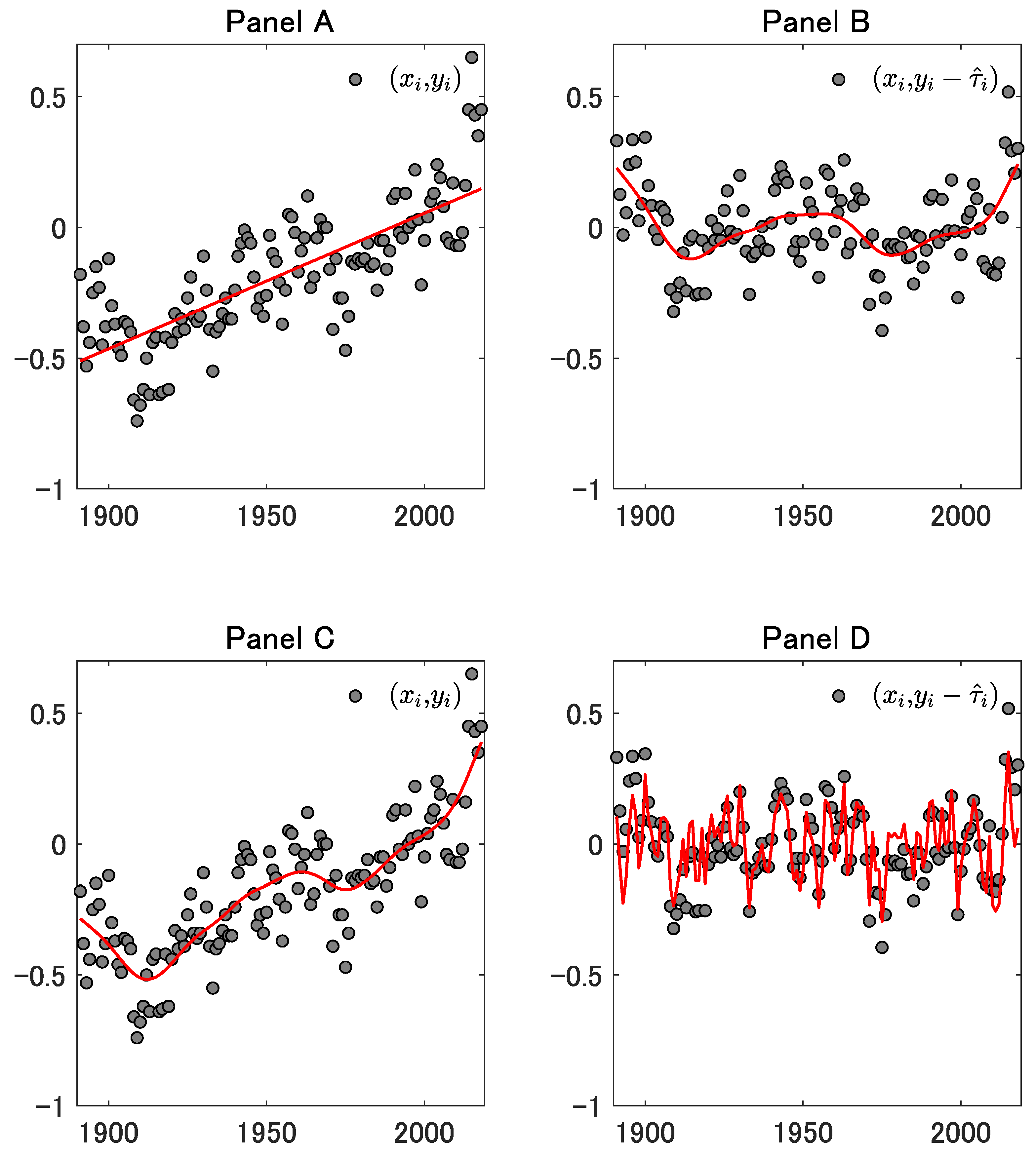
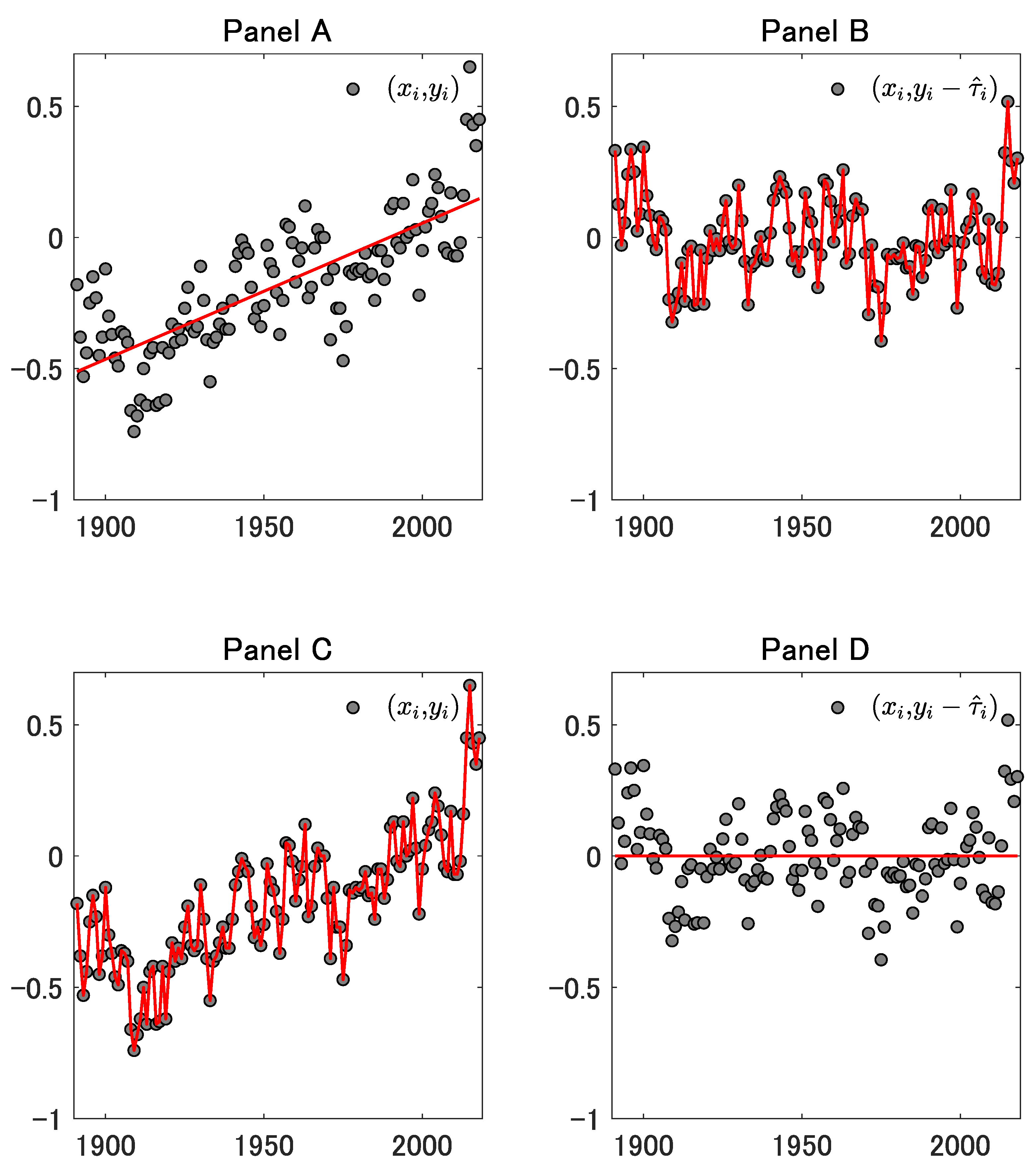
5. Illustrations of Some Results

In this section, we illustrate some of the results in the previous sections by a real data example.

Panel A of Figure 1 shows a scatter plot of North Pacific sea surface temperature (SST) anomalies (1891–2018). SST is an essential climate variable and has been used for the detection of climate change. See, for example, Høyer and Karagali [7] and the references therein. We obtained the data from the website of the Japan Meteorological Agency. The solid line in the panel plots $(x_i,{\widehat{\tau }}_i)$ for $i=1,\dots ,n$, where $\widehat{\mathbf{\tau }}={[{\widehat{\tau }}_1,\dots ,{\widehat{\tau }}_n]}^{\top }$ in (4) and $n=128$. Panel B of Figure 1 depicts a scatter plot of $(x_i,y_i-{\widehat{\tau }}_i)$ for $i=1,\dots ,n$. The solid line in the panel plots $(x_i,{\widehat{c}}_i)$ for $i=1,\dots ,n$, where $\widehat{\mathit{c}}={[{\widehat{c}}_1,\dots ,{\widehat{c}}_n]}^{\top }$ is calculated by (18) with $\lambda ={10}^3$. The solid line in Panel C denotes $(x_i,{\widehat{f}}_i)$, where $\widehat{\mathit{f}}={[{\widehat{f}}_1,\dots ,{\widehat{f}}_n]}^{\top }$ is calculated by (14) with $\lambda ={10}^3$. Panel D illustrates a scatter plot of $(x_i,y_i-{\widehat{\tau }}_i)$ for $i=1,\dots ,n$. The solid line in the panel plots $(x_i,{\widehat{u}}_i)$ for $i=1,\dots ,n$, where $\widehat{\mathit{u}}={[{\widehat{u}}_1,\dots ,{\widehat{u}}_n]}^{\top }$ is calculated by (27) with $\lambda ={10}^3$. Figure 2, Figure 3 and Figure 4 correspond to the cases such that $\lambda ={10}^5,{10}^{10},{10}^{-10}$, respectively.

Figure 1. Panel A shows a scatter plot of North Pacific sea surface temperature anomalies (1891–2018). The solid line in the panel plots $(x_i,{\widehat{\tau }}_i)$ for $i=1,\dots ,n$, where $\widehat{\mathbf{\tau }}={[{\widehat{\tau }}_1,\dots ,{\widehat{\tau }}_n]}^{\top }$ in (4) and $n=128$. Panel B depicts a scatter plot of $(x_i,y_i-{\widehat{\tau }}_i)$ for $i=1,\dots ,n$. The solid line in the panel plots $(x_i,{\widehat{c}}_i)$ for $i=1,\dots ,n$, where $\widehat{\mathit{c}}={[{\widehat{c}}_1,\dots ,{\widehat{c}}_n]}^{\top }$ is calculated by (18) with $\lambda ={10}^3$. The solid line in Panel C denotes $(x_i,{\widehat{f}}_i)$, where $\widehat{\mathit{f}}={[{\widehat{f}}_1,\dots ,{\widehat{f}}_n]}^{\top }$ is calculated by (14) with $\lambda ={10}^3$. Panel D illustrates a scatter plot of $(x_i,y_i-{\widehat{\tau }}_i)$ for $i=1,\dots ,n$. The solid line in the panel plots $(x_i,{\widehat{u}}_i)$ for $i=1,\dots ,n$, where $\widehat{\mathit{u}}={[{\widehat{u}}_1,\dots ,{\widehat{u}}_n]}^{\top }$ is calculated by (27) with $\lambda ={10}^3$.

Figure 2. This figure corresponds to the case where $\lambda ={10}^5$. For the other explanations, see Figure 1.

Figure 3. This figure corresponds to the case where $\lambda ={10}^{10}$. For the other explanations, see Figure 1.

Figure 4. This figure corresponds to the case where $\lambda ={10}^{-10}$. For the other explanations, see Figure 1.

Recall that concerning $\mathit{y}$, $\widehat{\mathbf{\tau }}$, $\widehat{\mathit{c}}$, $\widehat{\mathit{f}}$, and $\widehat{\mathit{u}}$, the following equations hold:

$$\begin{array}{c}\widehat{\mathbf{\tau }}+\widehat{\mathit{c}}=\widehat{\mathit{f}},\widehat{\mathit{c}}+\widehat{\mathit{u}}=\mathit{y}-\widehat{\mathbf{\tau }},\underset{\lambda \to \infty }{lim}\widehat{\mathit{c}}=\mathbf{0},\underset{\lambda \to \infty }{lim}\widehat{\mathit{f}}=\widehat{\mathbf{\tau }},\\ \underset{\lambda \to \infty }{lim}\widehat{\mathit{u}}=\mathit{y}-\widehat{\mathbf{\tau }},\underset{\lambda \to 0}{lim}\widehat{\mathit{c}}=\mathit{y}-\widehat{\mathbf{\tau }},\underset{\lambda \to 0}{lim}\widehat{\mathit{f}}=\mathit{y},\underset{\lambda \to 0}{lim}\widehat{\mathit{u}}=\mathbf{0}.\end{array}$$

From Figure 1, Figure 2, Figure 3 and Figure 4, we can observe that these theoretical results are well illustrated in these figures. For example, from Panel D in Figure 4, we can observe that $\widehat{\mathit{u}}$ almost equals $\mathbf{0}$ when $\lambda ={10}^{-10}$.

6. The Cases Such That the Other Right-Inverse Matrices Are Used

In this section, we illustrate what happens if the other right-inverse matrices are used.

Let $\mathit{M}\in {\mathbb{R}}^{m\times n}$ be of full row rank. Recall that in this paper ${\mathit{M}}_{\mathrm{r}}^{-1}$ denotes ${\mathit{M}}^{\top }{\left(\mathit{M}{\mathit{M}}^{\top }\right)}^{-1}$, which is a right-inverse matrix of a full-row-rank matrix $\mathit{M}\in {\mathbb{R}}^{m\times n}$. Define a set of matrices

$$\begin{array}{c}\hfill {\mathsf{\Gamma }}_M=\{\mathsf{\Xi }\in {\mathbb{R}}^{n\times m}:\mathit{M}\mathsf{\Xi }={\mathit{I}}_m\}.\end{array}$$

${\mathsf{\Gamma }}_M$ denotes the set of right-inverse matrices of $\mathit{M}$ and accordingly ${\mathit{M}}_{\mathrm{r}}^{-1}$ belongs to ${\mathsf{\Gamma }}_M$.

Lemma 14.

$\mathit{N}={\mathit{M}}_{\mathrm{r}}^{-1}$ if and only if $\mathit{N}\in {\mathsf{\Gamma }}_M$ and $\mathcal{S}\left(\mathit{N}\right)=\mathcal{S}\left({\mathit{M}}^{\top }\right)$.

Proof of Lemma 14.

It is clear that if $\mathit{N}={\mathit{M}}_{\mathrm{r}}^{-1}$, then $\mathit{N}\in {\mathsf{\Gamma }}_M$ and $\mathcal{S}\left(\mathit{N}\right)=\mathcal{S}\left({\mathit{M}}^{\top }\right)$. Conversely, suppose that $\mathit{N}\in {\mathsf{\Gamma }}_M$ and $\mathcal{S}\left(\mathit{N}\right)=\mathcal{S}\left({\mathit{M}}^{\top }\right)$. Then, $\mathit{M}\mathit{N}={\mathit{I}}_m$ and there exists a nonsingular matrix $\mathsf{\Sigma }\in {\mathbb{R}}^{m\times m}$ such that $\mathit{N}={\mathit{M}}^{\top }\mathsf{\Sigma }$. By removing $\mathit{N}$ from these equations, we have $\mathsf{\Sigma }={\left(\mathit{M}{\mathit{M}}^{\top }\right)}^{-1}$, which leads to $\mathit{N}={\mathit{M}}^{\top }{\left(\mathit{M}{\mathit{M}}^{\top }\right)}^{-1}={\mathit{M}}_{\mathrm{r}}^{-1}$. □

From Lemma 14, if $\mathit{N}\ne {\mathit{M}}_{\mathrm{r}}^{-1}$, then $\mathit{N}\notin {\mathsf{\Gamma }}_M$ or $\mathcal{S}\left(\mathit{N}\right)\ne \mathcal{S}\left({\mathit{M}}^{\top }\right)$. Accordingly, we have the following result:

Proposition 3.

If $\mathit{N}\in {\mathsf{\Gamma }}_M\backslash \left\{{\mathit{M}}_{\mathrm{r}}^{-1}\right\}$, then $\mathcal{S}\left(\mathit{N}\right)\ne \mathcal{S}\left({\mathit{M}}^{\top }\right)$.

Based on the result, we illustrate what happens if the other right-inverse matrices are used. We give an example. Let $\mathit{Z}\in {\mathsf{\Gamma }}_D\backslash \left\{{\mathit{D}}_{\mathrm{r}}^{-1}\right\}$. Then, from Proposition 3 and Lemma 3, it follows that $\mathcal{S}\left(\mathit{Z}\right)\ne \mathcal{S}\left({\mathit{D}}_{\mathrm{r}}^{-1}\right)={\mathcal{S}}^{\perp }\left(\mathsf{\Pi }\right)$. Accordingly, letting $\mathit{L}=[\mathsf{\Pi },\mathit{Z}]$, it follows that ${\mathit{Z}}^{\top }\mathsf{\Pi }\ne \mathbf{0}$ and $\mathit{D}\mathit{L}=[\mathit{D}\mathsf{\Pi },\mathit{D}\mathit{Z}]=[\mathbf{0},{\mathit{I}}_{n-2}]$. In addition, given that $\mathit{D}\mathsf{\Pi }=\mathbf{0}$, $\mathit{D}\mathit{Z}={\mathit{I}}_{n-2}$, and $\mathsf{\Pi }$ is of full column rank, $\mathit{L}$ is nonsingular. Thus, from [8], for example, we have

$$\begin{array}{c}\hfill \widehat{\mathit{f}}=\mathit{L}{({\mathit{L}}^{\top }\mathit{L}+\lambda {\mathit{L}}^{\top }{\mathit{D}}^{\top }\mathit{D}\mathit{L})}^{-1}{\mathit{L}}^{\top }\mathit{y}=\mathsf{\Pi }\widehat{\mathbf{\pi }}+\mathit{Z}\widehat{\mathbf{\epsilon }},\end{array}$$

(62)

where

$$\begin{array}{c}\hfill \widehat{\mathbf{\pi }}=\arg \underset{\mathbf{\pi }\in {\mathbb{R}}^2}{min}{\parallel (\mathit{y}-\mathit{Z}\widehat{\mathbf{\epsilon }})-\mathsf{\Pi }\mathbf{\pi }\parallel }^2={\left({\mathsf{\Pi }}^{\top }\mathsf{\Pi }\right)}^{-1}{\mathsf{\Pi }}^{\top }(\mathit{y}-\mathit{Z}\widehat{\mathbf{\epsilon }})\end{array}$$

(63)

and

$$\begin{array}{cc}\hfill \widehat{\mathbf{\epsilon }}& =\arg \underset{\mathbf{\epsilon }\in {\mathbb{R}}^{n-2}}{min}\parallel {\mathit{Q}}_{\mathsf{\Pi }}\mathit{y}-{\mathit{Q}}_{\mathsf{\Pi }}{\mathit{Z}\mathbf{\epsilon }\parallel }^2+\lambda {\parallel \mathbf{\epsilon }\parallel }^2\hfill \\ \hfill & ={({\mathit{Z}}^{\top }{\mathit{Q}}_{\mathsf{\Pi }}\mathit{Z}+\lambda {\mathit{I}}_{n-2})}^{-1}{\mathit{Z}}^{\top }{\mathit{Q}}_{\mathsf{\Pi }}\mathit{y},\hfill \end{array}$$

(64)

which shows that we may obtain (penalized) regressions relating to the cubic smoothing spline even if we use the other right-inverse matrices of $\mathit{D}$ such that $\mathit{Z}\in {\mathsf{\Gamma }}_D\backslash \left\{{\mathit{D}}_{\mathrm{r}}^{-1}\right\}$. Nevertheless, as illustrated here, they are more complex than those shown in Table 1 and Table 2.

7. Concluding Remarks

In this paper, we provided a comprehensive list of penalized least squares regressions relating to the cubic smoothing spline, and then revealed a principle of duality in them. This is the main contribution of this study. Such penalized regressions are tabulated in Table 1 and Table 2 and the principle of duality revealed is stated in Proposition 2. In addition, we also provided a number of results derived from them, most of which are also tabulated in Table 1 and Table 2 and some of which are illustrated in Figure 1, Figure 2, Figure 3 and Figure 4.

Appendix A.1. Some Remarks on a Special Case Such That x = [1,…,n]^⊤

(i)

If $\mathit{x}={[1,\dots ,n]}^{\top }$, then $\mathit{C}={\mathit{D}}_{\left(2\right)}{\mathit{D}}_{\left(1\right)}\in {\mathbb{R}}^{(n-2)\times n}$, which is a Toeplitz matrix of which the first (resp. last) row is $[1,-2,1,0,\dots ,0]$ (resp. $[0,\dots ,0,1,-2,1]$).

(ii)

If $\mathit{x}={[1,\dots ,n]}^{\top }$, then ${({\mathit{I}}_n+\lambda {\mathit{C}}^{\top }{\mathit{R}}^{-1}\mathit{C})}^{-1}$ is bisymmetric (i.e., symmetric centrosymmetric), which may be proved as in Yamada (2020a).

(iii)

If $\mathit{x}={[1,\dots ,n]}^{\top }$, then $\mathit{R}$ in (8) is not only a symmetric tridiagonal matrix but also a Toeplitz matrix. In the case, we have

$$\begin{array}{c}\hfill {\omega }_k=\frac{2}{3}+\frac{1}{3}cos\left(\frac{k\pi }{n-1}\right),k=1,\dots ,n-2,\end{array}$$

(A1)

and thus ${\omega }_{n-2}$, which is the smallest eigenvalue of $\mathit{R}$, satisfies the following inequality (see, e.g., [9]):

$$\begin{array}{c}\hfill {\omega }_{n-2}=\frac{2}{3}+\frac{1}{3}cos\left(\frac{n-2}{n-1}\pi \right)>\frac{1}{3}.\end{array}$$

(A2)

(iv)

If $\mathit{x}={[1,\dots ,n]}^{\top }$ and $\mathit{R}={\mathit{I}}_{n-2}$ in (2) and (3), then (2) and (3) reduce to

$$\begin{array}{cc}\hfill \widehat{\mathit{f}}& =\arg \underset{\mathit{f}\in {\mathbb{R}}^n}{min}{\parallel \mathit{y}-\mathit{f}\parallel }^2+{\parallel {\mathit{D}}_{\left(2\right)}{\mathit{D}}_{\left(1\right)}\mathit{f}\parallel }^2\hfill \\ \hfill & ={\left\{{\mathit{I}}_n+\lambda {\left({\mathit{D}}_{\left(2\right)}{\mathit{D}}_{\left(1\right)}\right)}^{\top }\left({\mathit{D}}_{\left(2\right)}{\mathit{D}}_{\left(1\right)}\right)\right\}}^{-1}\mathit{y}.\hfill \end{array}$$

(A3)

It is a type of the Whittaker–Henderson (WH) method of graduation, which was developed by Bohlmann [10], Whittaker [11] and others. See Weinert [12] for a historical review of the WH method of graduation. (A3) is also referred to as the Hodrick–Prescott (HP) [13] filtering in econometrics. For more details about the HP filtering, see, for example, Schlicht [14], Kim et al. [15], Paige and Trindade [16], and Yamada [17,18,19,20,21].

Appendix A.2. User-Defined Functions

Appendix A.2.1. A Matlab/GNU Octave Function to Make $\mathit{C}$ in (7)

Appendix A.2.2. A Matlab/GNU Octave Function to Make $\mathit{R}$ in (8)

Appendix A.2.3. A Matlab/GNU Octave Function to Make $\mathit{D}$ in (9)

Appendix A.2.4. A R Function to Make $\mathit{C}$ in (7)

Appendix A.2.5. A R Function to Make $\mathit{R}$ in (8)

Appendix A.2.6. A R Function to Make $\mathit{D}$ in (9)

References

- Schoenberg, I.J. Spline functions and the problem of graduation. Proc. Natl. Acad. Sci. USA 1964, 52, 947–950. [Google Scholar] [CrossRef] [PubMed]
- Reinsch, C. Smoothing by spline functions. Numer. Math. 1967, 10, 177–183. [Google Scholar] [CrossRef]
- Green, P.J.; Silverman, B.W. Nonparametric Regression and Generalized Linear Models: A roughness Penalty Approach; Chapman and Hall/CRC: Boca Raton, FL, USA, 1994. [Google Scholar]
- Wood, S.N. Generalized Additive Models: An Introduction with R, 2nd ed.; Chapman & Hall/CRC: Boca Raton, FL, USA, 2017. [Google Scholar]
- Hoerl, A.E.; Kennard, R.W. Ridge regression: Biased estimation for nonorthogonal problems. Technometrics 1970, 12, 55–67. [Google Scholar] [CrossRef]
- Verbyla, A.P.; Cullis, B.R.; Kenward, M.G.; Welham, S.J. The analysis of designed experiments and longitudinal data by using smoothing splines. J. R. Stat. Soc. 1999, 48, 269–311. [Google Scholar] [CrossRef]
- Høyer, J.L.; Karagali, I. Sea surface temperature climate data record for the North Sea and Baltic Sea. J. Clim. 2016, 29, 2529–2541. [Google Scholar] [CrossRef]
- Yamada, H. The Frisch–Waugh–Lovell theorem for the lasso and the ridge regression. Commun. Stat. Theory Methods 2017, 46, 10897–10902. [Google Scholar] [CrossRef]
- Pesaran, M.H. Exact maximum likelihood estimation of a regression equation with a first-order moving-average error. Rev. Econ. Stud. 1973, 40, 529–535. [Google Scholar] [CrossRef]
- Bohlmann, G. Ein ausgleichungsproblem. Nachrichten von der Gesellschaft der Wissenschaften zu Gottingen, Mathematisch-Physikalische Klasse 1899, 1899, 260–271. [Google Scholar]
- Whittaker, E.T. On a new method of graduation. Proc. Edinb. Math. Soc. 1923, 41, 63–75. [Google Scholar] [CrossRef]
- Weinert, H.L. Efficient computation for Whittaker–Henderson smoothing. Comput. Stat. Data Anal. 2007, 52, 959–974. [Google Scholar] [CrossRef]
- Hodrick, R.J.; Prescott, E.C. Postwar U.S. business cycles: An empirical investigation. J. Money Credit. Bank. 1997, 29, 1–16. [Google Scholar] [CrossRef]
- Schlicht, E. Estimating the smoothing parameter in the so-called Hodrick–Prescott filter. J. Jpn. Stat. Soc. 2005, 35, 99–119. [Google Scholar] [CrossRef]
- Kim, S.; Koh, K.; Boyd, S.; Gorinevsky, D. ℓ1 trend filtering. SIAM Rev. 2009, 51, 339–360. [Google Scholar] [CrossRef]
- Paige, R.L.; Trindade, A.A. The Hodrick–Prescott filter: A special case of penalized spline smoothing. Electron. J. Stat. 2010, 4, 856–874. [Google Scholar] [CrossRef]
- Yamada, H. Ridge regression representations of the generalized Hodrick–Prescott filter. J. Jpn. Stat. Soc. 2015, 45, 121–128. [Google Scholar] [CrossRef]
- Yamada, H. Why does the trend extracted by the Hodrick–Prescott filtering seem to be more plausible than the linear trend? Appl. Econ. Lett. 2018, 25, 102–105. [Google Scholar] [CrossRef]
- Yamada, H. Several least squares problems related to the Hodrick–Prescott filtering. Commun. Stat. Theory Methods 2018, 47, 1022–1027. [Google Scholar] [CrossRef]
- Yamada, H. A note on Whittaker–Henderson graduation: Bisymmetry of the smoother matrix. Commun. Stat. Theory Methods 2020, 49, 1629–1634. [Google Scholar] [CrossRef]
- Yamada, H. A smoothing method that looks like the Hodrick–Prescott filter. Econom. Theory 2020. [Google Scholar] [CrossRef]
Publisher’s Note: MDPI stays neutral with regard to jurisdictional claims in published maps and institutional affiliations. |
© 2020 by the authors. Licensee MDPI, Basel, Switzerland. This article is an open access article distributed under the terms and conditions of the Creative Commons Attribution (CC BY) license (http://creativecommons.org/licenses/by/4.0/).