Nonlinear Dynamics and Control of a Cube Robot

Abstract

The paper aims to solve problems of the mathematical modeling and realization of a cube robot capable of self-bouncing and self-balancing. First, the dynamic model of the cube robot is derived by using the conservation of the angular momentum and the torque equilibrium theory. Furthermore, the controllability of the cube robot is analyzed and the angle of the cube robot is derived from the attitude and heading reference system (AHRS). Then the parallel proportional–integral–derivative (PID) controller is proposed for the balancing control of the self-designed cube robot. As for the bounce control of the cube robot, a braking system triggered by the servo motor is designed for converting the kinetic energy to the potential energy. Finally, the experimental results are included to demonstrate that the cube robot can complete the actions of self-bouncing and self-balancing with good robustness to external disturbances.

1. Introduction

The cube robot is a cube-shaped system with an embedded reaction wheel generating the control torque to complete self-balancing and self-bouncing actions. The mathematical model of the cube robot is a typical nonlinear dynamic system. In addition, the system is an unstable and multi-dimensional inverted pendulum. Therefore, we need to design an appropriate controller to generate a corresponding torque inside the cube robot to maintain its balance. In 2012, a cube robot called Cubli was designed and driven by the inner reaction wheel fixed on the cube’s three faces [1]. The balancing controller design is always challenging due to the cube robot’s modeling problem and complexity. The linear-quadratic regulator (LQR) control algorithm for the Cubli balancing on its edge and corner was conducted in [2]. In 2017, Chen et al. [3] proposed methods to construct the dynamic model of a self-balancing cube robot and a proportional–integral–derivative (PID) controller was proposed to accomplish the action of the cube robot balancing [4]. However, the cube robot mentioned above did not provide the dynamic model. The methodology for realizing the cube robot’s action of bouncing and balancing is not clearly described. In [5], a balance controller based on sliding mode control (SMC) is proposed. In the cube robot prototype, the SMC and PID controller are compared through numerical simulations and the conclusion is that the performance of SMC is better than that of the PID controller. Tian [6] introduced the concept of fuzzy control to design the balancing controller. Muehlebach et al. [7] studied the cubical robot’s balancing control based on the back-stepping method. However, the results in the works as mentioned above were available when the system was modeled correctly. On the other hand, the PID controller is a well-known popular control strategy and widely applied to solve the control problem in many industrial applications due to its simple structure and robust feature [8]. Many rules have been developed for tuning the optimal or sub-optimal PID controller gains [9,10]. Therefore, in this paper, we utilize the PID control approach to propose a new hardware mechanism different from that of [2] to achieve the balance and bounce control of the cube robot.

Three steps, including mathematical modeling, control, and system realization, should be addressed to complete the design and realization of a cube robot prototype capable of self-balancing and self-bouncing. First, to construct the model of the cube robot’s motion of bouncing up and self-balancing, this paper introduces the conservation of angular momentum theory and energy theory to obtain the dynamic model of the cube robot. After analyzing the dynamic system model, the state space equation and state variables can be obtained. In the proposed model, state variables are the angle of the cube robot, the cube robot’s angular velocity, and the velocity of the reaction wheel. Second, we use a 6-axis inertial measurement device to detect its acceleration and angular velocity. With these detected data, the cube robot’s angle can be derived from the attitude and heading reference system [11].

Furthermore, by applying the angle and angular velocity to the parallel PID controllers, the cube robot can balance on its edge. Third, we set up a combined solution of the multi-dimensional cube robot containing mechanical design, firmware architecture, and software development. And to accomplish the action of the cube robot bouncing, a braking system is constructed to stop the reaction wheel rotation such that the cube robot can bounce up. As for the firmware architecture, an IAR-embedded system is introduced to set up and implement the controller. The data is collected by using the embedded control panel STM32F407 with the function of the timer interrupt. We use Microsoft Visual Studio Professional 2013 platform and C programming language to develop the control software for the cube robot in software development. Figure 1 shows the cube robot designed in this paper balancing at its edge.

The framework of the paper is given as follows. Section 2 is the description of the cube robot prototype, including the mechanical structure and balancing equation. Section 3 is the estimation and control design for the proposed cube robot. The realization of the system and experimental results are included in Section 4 and Section 5, respectively. Section 6 is the conclusion.

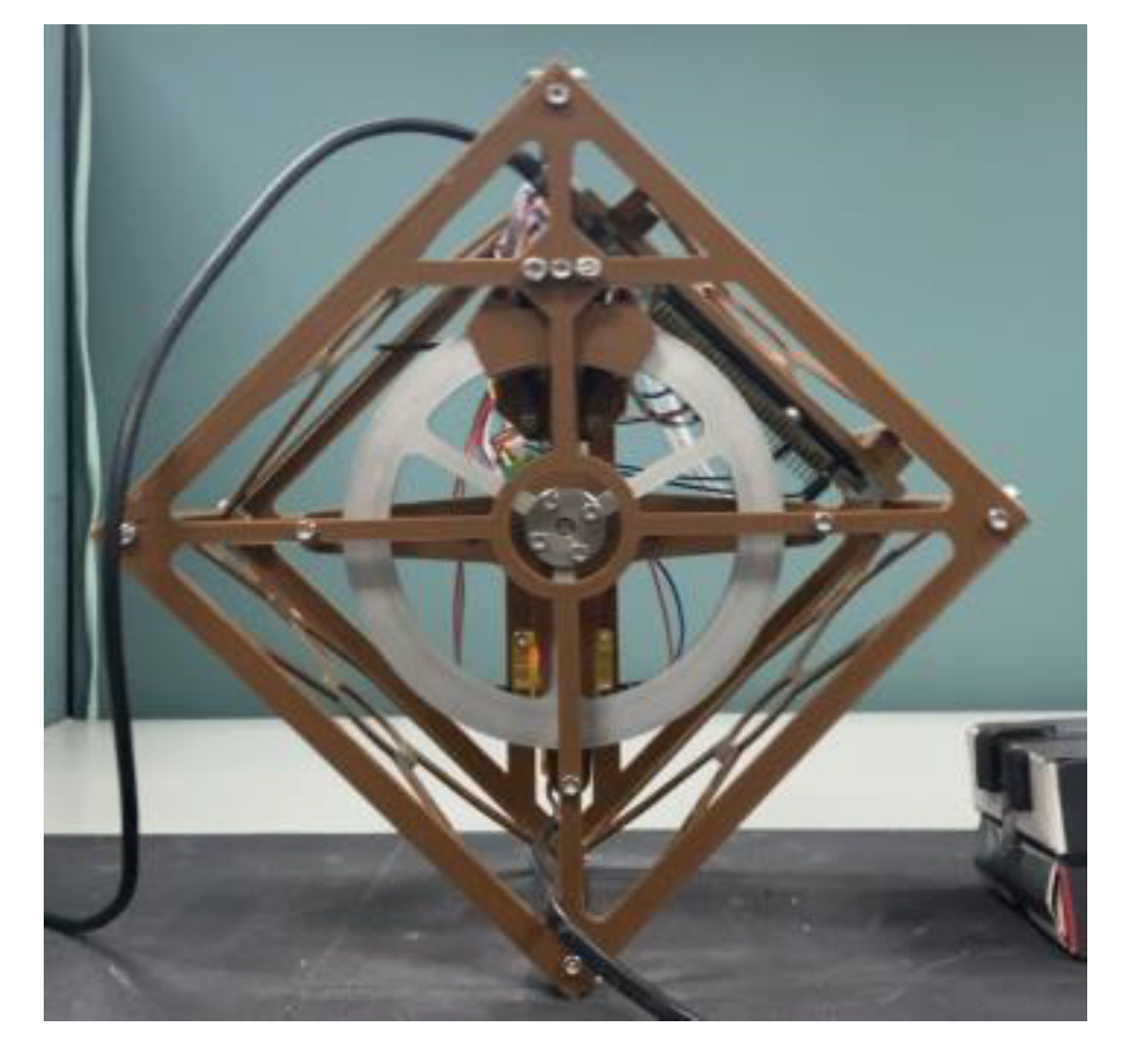
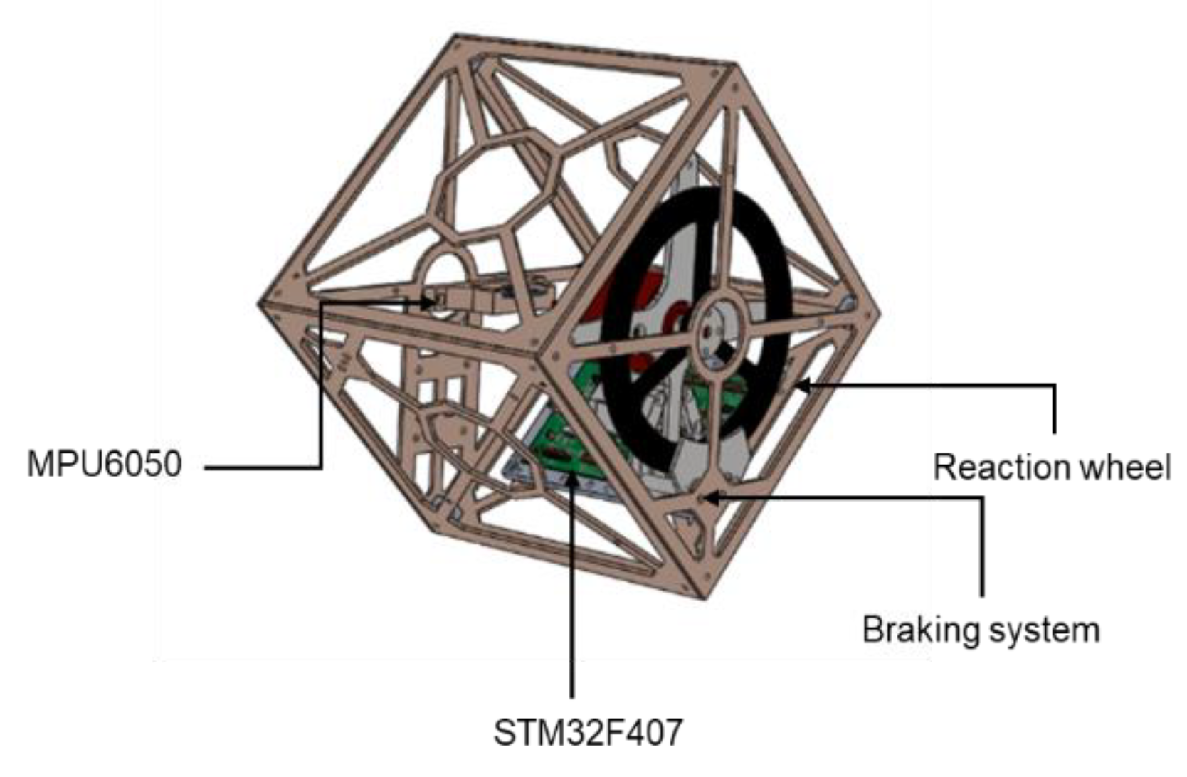
2. The Cube Robot Prototype

Figure 2 illustrates the cube robot prototype that consists of six-sided square plastic faces. One of the plastic faces holds the reaction wheel driven by the brushless motor at its center, and the braking system is fixed at its corner. Considering the strength of the plastic faces, each side of the cube’s thickness is designed to be 2 mm. Furthermore, to let the cube robot swing freely during the balancing, each face of the cube robot must be in a closed-state at the joint, which is shown in Figure 3.

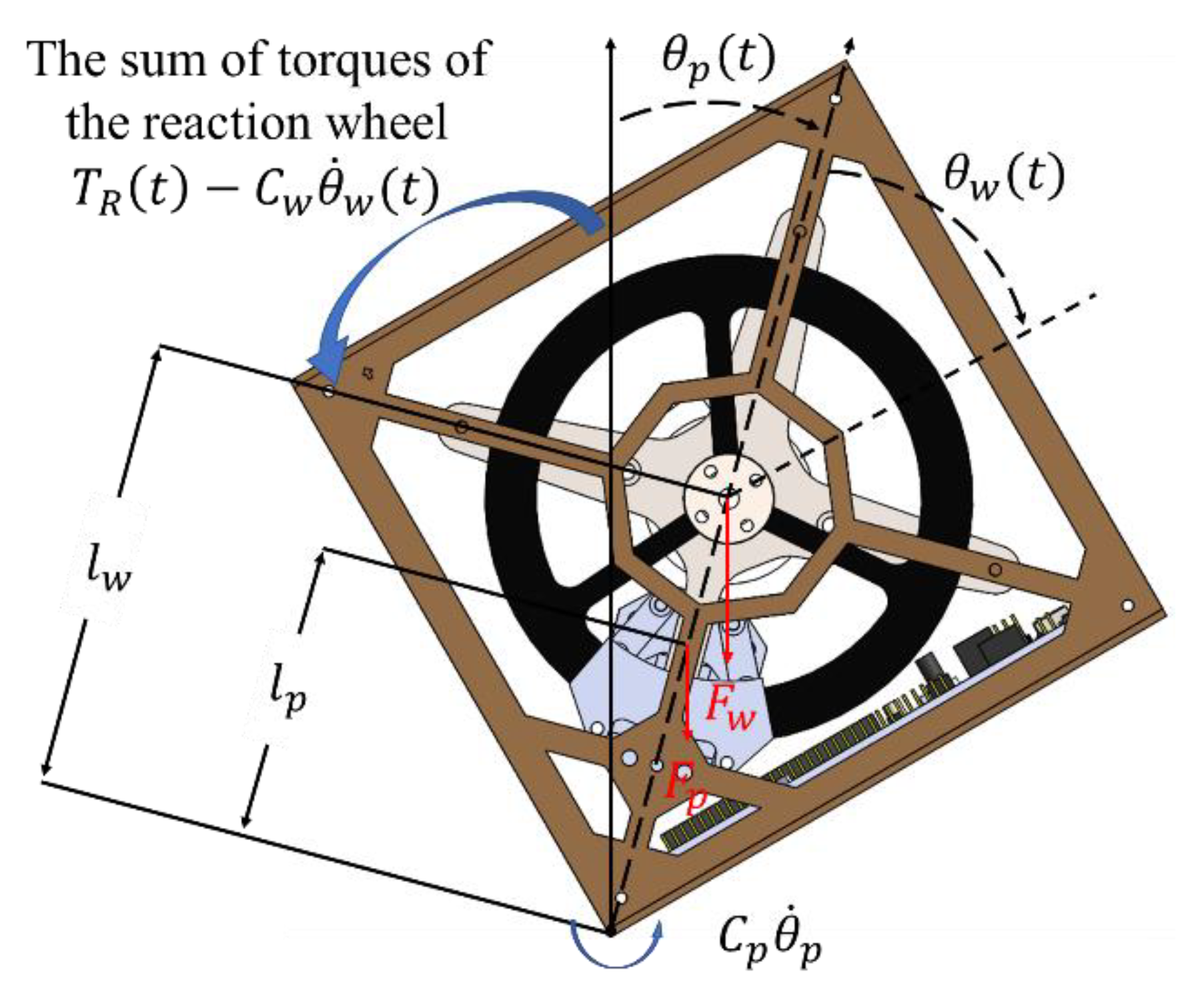
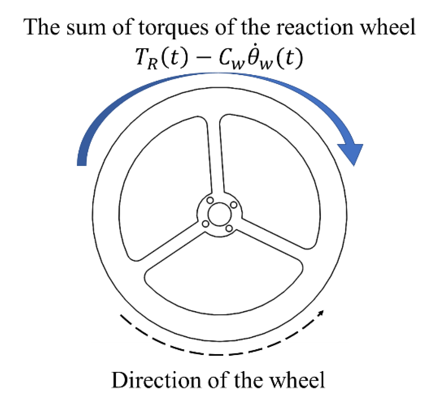
2.1. System Dynamics

The overall system consists of a cube robot, reaction wheel, servo motor, brushless motor, a braking system [12], and a control processor. The cubical robot’s edge is fixed with the axis, and the brushless motor is set on the center of the cubical robot’s single face. The concepts of torque and rotation angle are shown in Figure 4. The torque analysis of the internal reaction wheel driving the cube robot is shown in Figure 5. In Figure 4, $l_P$ denotes the distance from the cube robot’s center of gravity to the axis. $F_P$ is the cube robot’s gravity and $l_w$ denotes the distance from the reaction wheel’s center of the gravity to the axis. $F_W$ denotes the reaction wheel’s gravity, $C_W$ and $C_P$ represent the rotating axis friction coefficients of the cube robot and the reaction wheel, respectively, and $T_R(t)$ denotes the torque. The tilt angle of the cube robot is defined as ${\theta }_P(t)$ and the rotation angle of the reaction wheel is defined as ${\theta }_W(t)$. The torque, applying to the cube robot and reaction wheel, is the sum of the torques generated from the brushless motor and friction torque $C_W{\dot{\theta }}_W$, which is opposite to the reaction wheel rotation, as shown in Figure 5.

By applying the conservation of the angular momentum and torque equilibrium theory, the nonlinear dynamic equation of the cube robot shown in Figure 4. is given as:

$$\{\begin{array}{l}{M}_C^O(t)=I_C^O{\ddot{\theta }}_P(t)=F_P{l}_P\sin {\theta }_P(t)+F_W{l}_w\sin {\theta }_P(t)-T_R(t)-C_P{\dot{\theta }}_P(t)+C_W{\dot{\theta }}_W(t)\\ M_W(t)=I_W({\ddot{\theta }}_P(t)+{\ddot{\theta }}_W(t))=T_R(t)-C_W{\dot{\theta }}_W(t),\end{array}$$

(1)

where ${\dot{\theta }}_P$ is the angular velocity of the cube robot and ${\ddot{\theta }}_P$ is the angular acceleration of the cube robot. ${\dot{\theta }}_W$ is the angular velocity of the reaction wheel, and ${\ddot{\theta }}_W$ is the angular acceleration of the reaction wheel. $M_C^O$ is the sum of torques of the system at the axis and $M_W$ is the sum of torques of the reaction wheel.

The system’s moment of the cube robot is given below:

$$I_C^O=I_P^O+I_W^O=I_P^O+I_W+m_W{l}^2$$

(2)

where $I_C^O$ is the system’s moment of the inertia about the axis. $I_P^O$ is the moment of inertia of the cube robot’s body about the axis, while $I_W^O$ is the moment of the inertia of the reaction wheel about the axis and can be substituted with $I_W+m_W{l}^2$ based on the parallel axis theorem. $I_W$ is the moment of the inertia of the wheel. Moreover, we have $F_P=m_{P}g$ and $F_W=m_{w}g$, where $g$ is gravitational acceleration. Therefore, from Equations (1) and (2), the nonlinear balancing equation can be expressed by:

$$\{\begin{array}{l}{\ddot{\theta }}_P(t)=\frac{(m_P·l_P+m_w·l_w)g\sin {\theta }_P(t)-T_R(t)-C_P{\dot{\theta }}_P(t)+C_W{\dot{\theta }}_W(t)}{I_P^O+I_W+m_W{l}^2}\\ {\ddot{\theta }}_W(t)=\frac{T_R(t)-C_W{\dot{\theta }}_W(t)}{I_W}-{\ddot{\theta }}_P(t).\end{array}$$

(3)

Furthermore, the brushless motor generating the inner torque is driven with pulse width modulation (PWM) and the mathematical equation of the armature circuit can be expressed as follows:

$$v_a(t)=R_m·i_a(t)+L_a\frac{d{i}_a(t)}{dt}+K_{e}n\dot{\varnothing }(t)$$

(4)

where $K_e$ is the back electromotive force constant, $R_m$ is the armature resistance, $L_a$ is the armature inductance, $v_a(t)$ is the armature voltage, $i_a(t)$ is the armature current, and $\varnothing (t)$ is the magnetic flux. $n\dot{\varnothing }(t)$ is the angular velocity of the rotor and $n$ is the pulley ratio. Since the armature inductance $L_a$ is very small, the term $L_a\frac{\mathrm{d}{i}_a(t)}{\mathrm{d}t}$ in Equation (4) can be neglected, and then the input torque can be expressed by:

$$T_R(t)=K_t{i}_a(t)=\frac{K_t}{R_m}{\nu }_a(t)-n\frac{K_t{K}_e}{R_m}\dot{\varnothing }(t)$$

(5)

where $K_t$ is the moment constant of the motor.

From Equations (3)–(5), the balancing equation can be derived as:

$$\{\begin{array}{l}{\ddot{\theta }}_P(t)=\frac{(m_P·l_P+m_w·l_w)g\sin {\theta }_P(t)-\frac{K_t}{R_m}(v_a(t)-n{K}_e\dot{\varnothing }(t))-C_P{\dot{\theta }}_P(t)+C_W{\dot{\theta }}_W(t)}{I_P^O+I_W+m_W{l}_W^2}\\ {\ddot{\theta }}_W(t)=\frac{\frac{K_t}{R_m}(v_a(t)-n{K}_e\dot{\varnothing }(t))-C_W{\dot{\theta }}_W(t)}{I_W}-{\ddot{\theta }}_P(t).\end{array}$$

(6)

Table 1. System parameters.

Coefficient	Value
$g$ (m/s2)	9.81
$m_P$ (kg)	0.723
$m_w$ (kg)	0.162
$I_P^o$ (kg $·{\mathrm{m}}^2$)	$1.37\times {10}^{-2}$
$I_w$ (kg $·{\mathrm{m}}^2$)	$0.3267\times {10}^{-3}$
$l_w (\mathrm{m})$	0.11
$l_p (\mathrm{m})$	0.095
$C_P$ (kg $·{\mathrm{m}}^2·{\mathrm{s}}^2$)	$1.02\times {10}^{-3}$
$C_w$ (kg $·{\mathrm{m}}^2·{\mathrm{s}}^2$)	0.6 $\times {10}^{-3}$
$K_t$ (N $·\mathrm{m}·{\mathrm{A}}^{-1}$)	$38.6\times {10}^{-3}$
$R_m(\mathsf{\Omega })$	0.8158
$L_a$ (H)	3.6 × ${10}^{-3}$
$K_e$ (v $·{\mathrm{web}}^{-1}·\mathrm{s}$)	$1.78\times {10}^{-2}$
$n$	30

shows the parameters of the cube robot given in Figure 1. $K_t, K_e, R_m, L_a,n$ are obtained from the motor manufacturer (MABUCHI company, Chiba, Japan). $g$ = 9.81 m/s² is the gravitational acceleration. The other parameters can be obtained from the well-known Newton’s law of motion and the friction coefficient experiment.

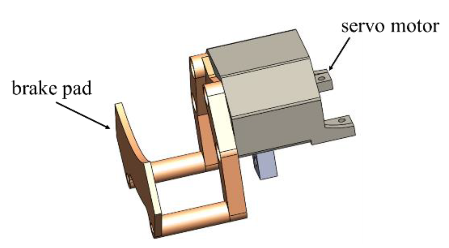
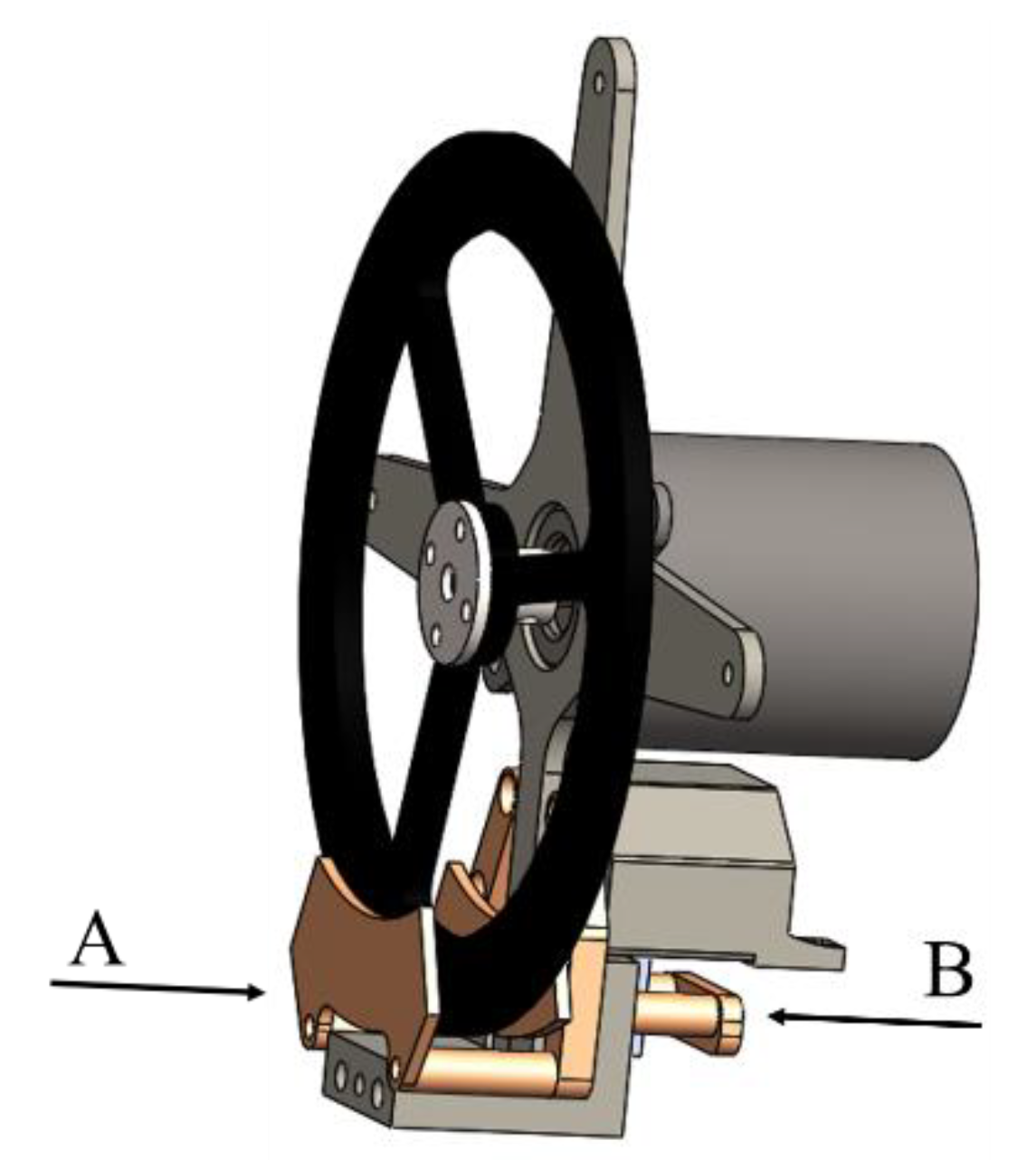
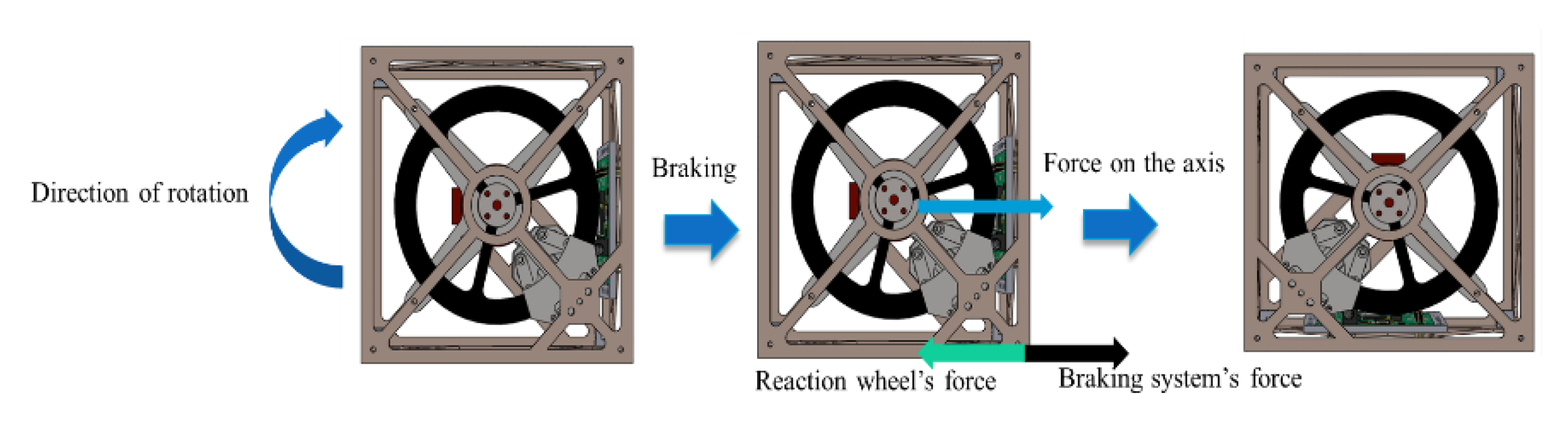
2.2. The Braking System

Figure 6 shows the braking system’s gadget where a servo motor is used to trigger the spring and let the brake pad push to the reaction wheel. The black arrow shows the placed position of the brake pad. Figure 7 shows the server motor of the braking system. The left arrow shows where the servo motor is placed. The right arrow shows where the brake pad is placed, which will move backward to collide with the reaction wheel.

The whole braking system is shown in Figure 8, with arrow A representing the direction of where the servo motor pushes and arrow B expressing the brake pad’s direction moving from another side. After the servo motor triggers the braking system, the brake pad attached to the gadget will collide with the reaction wheel. Thus, the design can stop the reaction wheel efficiently.

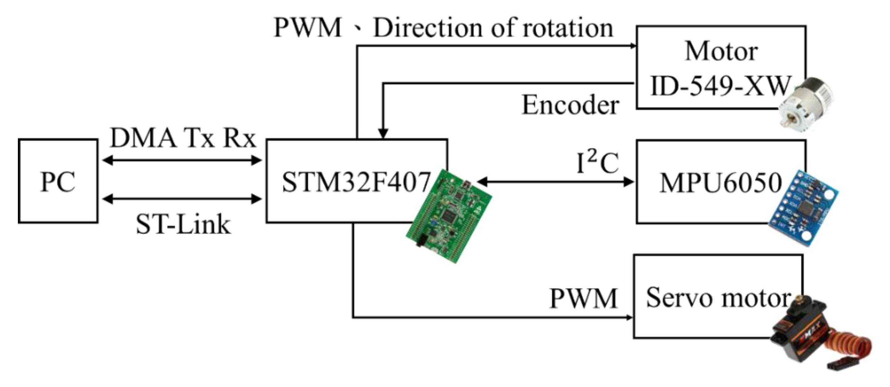
2.3. Signal Processing Units

Figure 9 shows the signal processing units of the cube robot. The STM32F407 evaluation board (which mounted a Cortex-M3 clocked at 72MHZ) is the primary system processing unit. The IMU sensor consists of a 3-axis accelerometer, ADXL345 made from Analog Devices, and a 3-axis gyro made from InvenSense. The IMU sensor that mounts on the cube robot’s backside is connected to the STM 32F407 board. And the serial communication between them is Inter-Integrated Circuit (${\mathrm{I}}^2\mathrm{C}$).

A 20 W brushless motor ID-549-XW made by MABUCHI company is chosen to drive the cube robot’s reaction wheel due to its simple control method and high efficiency compared to the brush motor. The optical encoder of the brushless motor is used to sense the velocity ${\dot{\theta }}_W$ of the reaction wheel. The brushless motor is driven by the PWM signal, which is generated from the STM32F407 board. The RC servo motor, ES08MAII, which triggers the braking system, is also driven by the pulse width modulation (PWM) signals.

The STM32 port of the timer interrupt is used as the software’s framework due to its high accuracy sampling time, which allows us to design the appropriate filter for the IMU sensor. Furthermore, to verify the robustness and stability of the cube robot, we use the peripheral in STM32F407 control panel, DMA, to collect the state parameter data such as the cube robot’s angle.

3. Estimation and Control

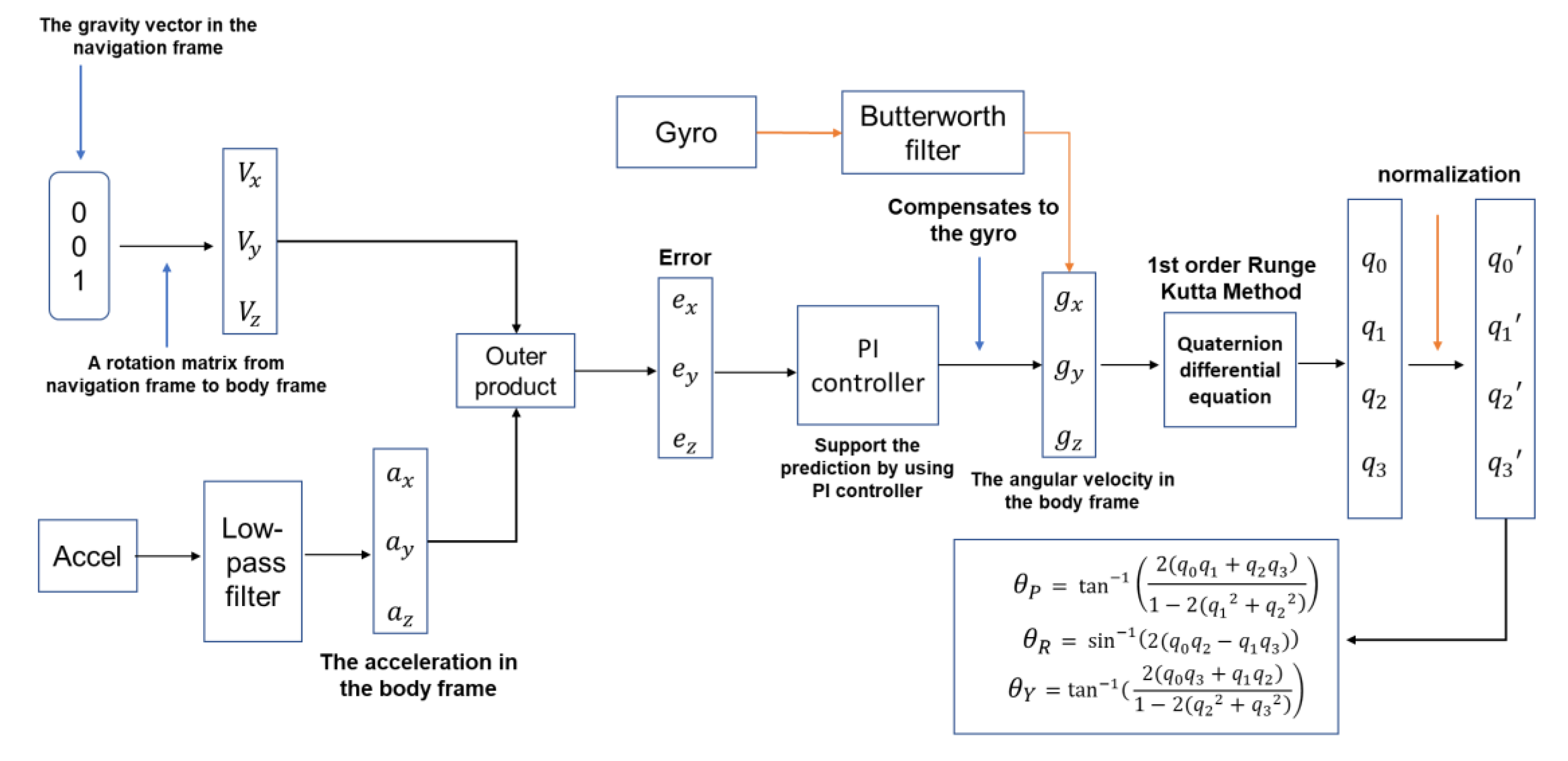
3.1. Attitude and Heading Reference System

The angle, angular velocity, and reaction wheel’s velocity are essential state variables of the cube robot. Thus, to acquire the rotation angle of the cube robot correctly, the pitch angle ${\theta }_P$, one of the variables of the Euler angle, and its angular velocity ${\dot{\theta }}_P$ are obtained by the gyro on the IMU sensors.

The Euler angle provides a way to represent the 3D orientation of an object by using a combination of three rotations about different axes. For instance, the rotation of the y-axis is described as Pitch, and the rotation of the z-axis is described as Yaw. Here, the quaternion is applied to estimate the Euler angles and to avoid the Gimbal lock effect [13]. The quaternion-derived rotation matrix can be expressed in terms of $q_i$ as follows [14,15]:

$$\left[\begin{array}{c}{q}_1^{\prime }\\ q_2^{\prime }\\ q_3^{\prime }\end{array}\right]=\left[\begin{array}{ccc}1-2({q_2}^2+{q_3}^2)& 2(q_1{q}_2-q_0{q}_3)& 2(q_0{q}_2+q_1{q}_3)\\ 2(q_1{q}_2+q_0{q}_3)& 1-2({q_1}^2+{q_3}^2)& 2(q_2{q}_3-q_0{q}_1)\\ 2(q_1{q}_3-q_0{q}_2)& 2(q_2{q}_3+q_0{q}_1)& 1-2({q_1}^2+{q_2}^2)\end{array}\right]\left[\begin{array}{c}{q}_1\\ q_2\\ q_3\end{array}\right]$$

(7)

where $q_i$, $i=1,2,3$ are the three directions of q, and q is a unit quaternion, $q_i^{\prime }$ $i=1,2,3$ are the three directions of $q^{\prime }$, and $q^{\prime }$ is the estimation of q.

After calculating the quaternion-derived rotation matrix, the Euler angle can be obtained from the quaternions via the above equation:

$$\begin{gathered} {\theta }_P={\tan }^{-1}(\frac{2(q_0{q}_1+q_2{q}_3)}{1-2({q_1}^2+{q_2}^2)}) \\ {\theta }_R={\sin }^{-1}(2(q_0{q}_2-q_1{q}_3)) \\ {\theta }_Y={\tan }^{-1}(\frac{2(q_0{q}_3+q_1{q}_2)}{1-2({q_2}^2+{q_3}^2)}) \end{gathered}$$

(8)

where ${\theta }_P$ denotes Pitch, ${\theta }_R$ denotes Roll, and ${\theta }_Y$ denotes Yaw. By using the relationship between the Euler angle and quaternion, the Pitch angle of the cube robot can be obtained.

The quaternion inside the rotation matrix will have drift error after long-term usage. To avoid that, the system needs to constantly update the quaternion using the one-order Runge–Kutta method [16]. The equation of the one-order Runge–Kutta is shown below:

$$Q_{t+T_d}=Q_t+\frac{T_d}{2}·\frac{dQ}{dt}$$

(9)

where $Q_t={\left[q_0 q_1 q_2 q_3\right]}_t^T$ denotes the initial status of the quaternion, $\frac{dQ}{dt}$ denotes the derivative of the quaternion $Q_t$ at the time $t$, and the $Q_{t+T_d}$ denotes the estimation of the quaternion $Q_t$ at the time $t+T_d$. $T_d>0$ is the sampling time.

After applying the Runge–Kutta method, the equation of the quaternion updated can be derived as:

$$\left[\begin{array}{c}{q}_0^{\prime }\\ q_1^{\prime }\\ q_2^{\prime }\\ q_3^{\prime }\end{array}\right]={\left[\begin{array}{c}{q}_0\\ q_1\\ q_2\\ q_3\end{array}\right]}_{t+T_d}={\left[\begin{array}{c}{q}_0\\ q_1\\ q_2\\ q_3\end{array}\right]}_t+\left[\begin{array}{c}-{\omega }_x{q}_1-{\omega }_y{q}_2-{\omega }_z{q}_3\\ {\omega }_x{q}_0+{\omega }_z{q}_2-{\omega }_y{q}_3\\ {\omega }_y{q}_0-{\omega }_z{q}_1-{\omega }_x{q}_3\\ {\omega }_z{q}_0+{\omega }_y{q}_1-{\omega }_x{q}_2\end{array}\right]\frac{T_d}{2}$$

(10)

where ${\omega }_x, {\omega }_y$, and ${\omega }_z$ denote the angular velocity of the three axes x, y, and z, respectively.

Figure 10 illustrates how the attitude and heading reference system operates in the cube robot. First, the acceleration and angular velocity values sensed by MPU6050 are filtered by a low-pass filter. Second, the vector in the navigation frame is then converted into the body frame by using the quaternion matrix. Using the outer product, the error of the gravity vector between the body frame and navigation frame can be calculated. Third, a proper PI controller is used to support the prediction while responding to the high-frequency changes in the error [16]. After calculating the error, we compensate for the gyro error and use the quaternion differential equation to update the quaternion. At last, the cube robot angel, ${\theta }_P$, can be calculated via the relationship between the quaternion and Euler angle.

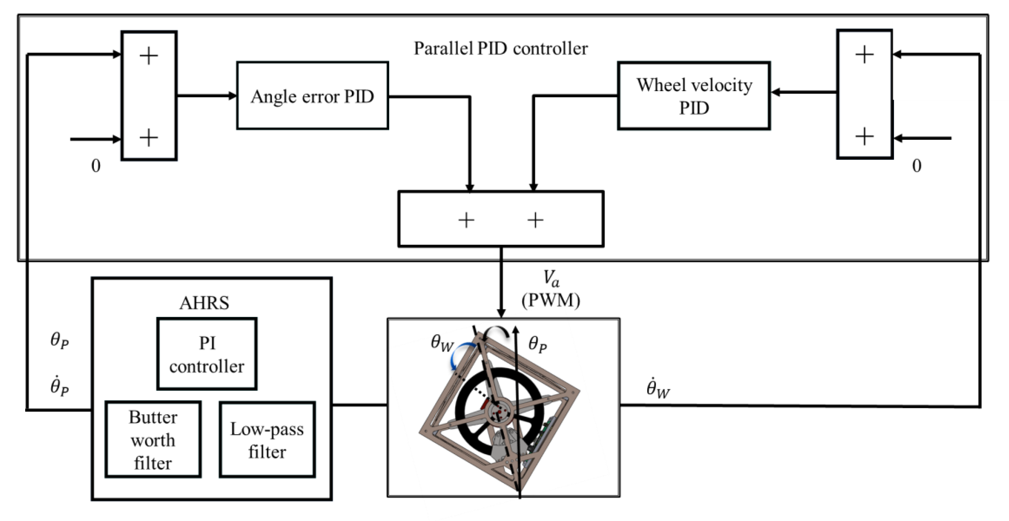
3.2. Balancing Control

After linearization Equation (3) at the equilibrium point ${\theta }_P=0^{°}$, the dynamic equation can be represented by the state space formula:

$$\dot{x}(t)=Ax(t)+Bu(t)$$

(11)

where $x(t)={\left[{\theta }_P(t), {\dot{\theta }}_P(t), {\dot{\theta }}_W(t)\right]}^T$ is a vector of state variables, and A, B are the system matrices defined below:

$$\begin{array}{l}A=\left[\begin{array}{ccc}0& 1& 0\\ \frac{(m_P{l}_P+m_W{l}_W)g}{I_P^o+I_W+m_W{l_W}^2}& \frac{-C_P}{I_P^o+I_W+m_W{l_W}^2}& \frac{C_W}{I_P^o+I_W+m_W{l_W}^2}\\ -\frac{(m_P{l}_P+m_W{l}_W)g}{I_P^o+I_W+m_W{l_W}^2}& \frac{C_P}{I_P^o+I_W+m_W{l_W}^2}& \frac{-C_W(I_P^o+2I_W+m_W{l_W}^2)}{I_P^o+I_W+m_W{l_W}^2}\end{array}\right]\\ B=\left[\begin{array}{c}0\\ \frac{-K_t}{I_P^o+I_W+m_W{l_W}^2}\\ \frac{-K_t(I_P^o+I_W+m_W{l_W}^2)}{I_W(I_P^o+I_W+m_W{l_W}^2)}\end{array}\right]\end{array}$$

(12)

After calculating the state-space model, we can determine whether the cube robot’s model is controllable.

3.3. System Controllability

To verify the system’s controllability, the continuous-time controllability matrix [17] can be obtained by using the parameters in Table 1 and the Equation (12). The matrix is shown as:

$$W_c=\left[\begin{array}{ccc}0.001& 0& -0.003\\ 0& 0.2367& -3.8605\\ -0.003& -3.8605& 65.3239\end{array}\right]$$

(13)

and its eigenvalues are:

$$\mathrm{eig}(W_c)=\left[\begin{array}{ccc}0.0001& 0.0085& 65.5521\end{array}\right]$$

(14)

and the corresponding eigenvectors $v_1,v_2,v_3$ are:

$$\left[v_1,v_2,v_3\right]=\left[\begin{array}{ccc}-0.9997& -0.0245& 0\\ 0.0245& 0.998& -0.0591\\ 0.0015& 0.0591& 0.9983\end{array}\right]$$

(15)

The rank of a matrix $W_c$ is 3, which implies that the system is fully controllable. According to reference [18], the smaller the eigenvalue $0.0001$, the larger the input energy will be needed to drive the system from the arbitrary state to the state of its corresponding eigenvector $v_1$. As the eigenvalues are shown above, the velocity of the reaction wheel ${\dot{\theta }}_W$ has the biggest eigenvalue $65.5521$ in the continuous-time controllability gramian matrix. This means that the corresponding eigenvector to the biggest eigenvalue is the most controllable direction in state space [19]. In other words, the system will have a greater change in the direction of the state parameters, ${\dot{\theta }}_W$, on the same input energy compared to the other two state variables. This is the exact reason why the state variable ${\dot{\theta }}_W$ needs a parallel controller to balance the cube robot.

3.4. System Controller

The solution of the state space Equation (11) can be derived as:

$$x(t)=e^{A(t-t_0)}x(t_0)+{{\displaystyle \int }}_{t_0}^t{e}^{A(t-\tau )}Bu(\tau )d\tau .$$

(16)

Let the initial time $t_0=k{T}_d$, $t=k{T}_d+T_d$, the equation can be derived as:

$$x(k{T}_d+T_d)=e^{A(T_d)}x(k{T}_d)+{{\displaystyle \int }}_{k{T}_d}^{k{T}_d+T_d}{e}^{A(k{T}_d+T_d-\tau )}Bu(\tau )d\tau .$$

(17)

By normalizing the sampling time $T_d=1$, the continuous-time system given by Equation (12) can be discretized by sampling and zero-order hold. Then the discrete-time model is given below:

$$x\left[k+1\right]=A_{d}x\left[k\right]+B_{d}u\left[k\right], k\in {\mathbb{N}}_0$$

$$A_d=e^{A{T}_d}=I+\frac{A{T}_d}{2!}+\frac{{(A{T}_d)}^2}{3!}\cdots$$

$$B_d={{\displaystyle \int }}_0^{T_d}{e}^{A\rho }d\rho ·B$$

Therefore, we have:

$$\begin{gathered} A_d=\left[\begin{array}{ccc}1.0321& 0.0202& 0\\ 3.23& 1.0283& 0.0002\\ -3.2249& -0.0282& 0.9967\end{array}\right] \\ {B}_d=\left[\begin{array}{c}-0.0015\\ -0.1467\\ 2.5552\end{array}\right]. \end{gathered}$$

(18)

$A_d$ and $B_d$ represent the system matrix of discrete-time, corresponding to the system matrix $A$ and $B$ of continuous-time. For the discrete-time system of Equation (18), a discrete-time PID controller is designed as:

$$u(k)=K_{P}e(k)+K_i{\displaystyle \sum }_{i=0}^{k}e(i)+K_d\left[e(k)-e(k-1)\right]$$

(19)

where $u(k)$ is the input at the sampling time k, $e(k)$ is the error at the sampling time status $k$, $e(k-1)$ is the error at the sampling time $(k-1),$ and ${\displaystyle \sum }_{i=0}^{k}e(i)$ is the summation of the error from sampling time 0 to $k$. $K_P$, $K_i$, and $K_d$ are the parameters of the discrete-time PID controller. Figure 11 illustrates the parallel PID controller structure designed to balance the cube robot.

To balance the robot, two kinds of PID controllers, including angle balance controller and wheel velocity controller, are processing the control signal at the same time in parallel to achieve the balance. The angle error PID controller aims at the control of the robot angle ${\theta }_P$. The wheel velocity PID controller is used to control the angular velocity of the reaction wheel (or the brushless motor). Based on the cube robot’s system parameters given in Table 1, the parameters of the proposed parallel PID are given in Equation (20). Moreover, the system disturbance and sensor fusion will influence the acceleration and angular velocity measurements’ accuracy. Thus, to reduce the low-frequency noise, we apply a one order Low-pass filter on the acceleration detection. The cut-off frequency of the low pass filter is 25 Hz, and the sampling frequency is 200 Hz. Furthermore, to increase the smoothness and reduce the low-frequency noise, we apply a second-order butterworth filter on the detection of the angular velocity. The cut-off frequency of the butter worth filter is 40 Hz, and the sampling frequency is 200 Hz. The parameters of the PID controller and coefficient of the filters and PI controller in Figure 11 can be designed as:

Parallel PID controller:

$$\begin{gathered} \mathrm{Angle}\mathrm{error}\mathrm{PID}:K_P=890, K_I=0.01, K_D=53.2 \\ \mathrm{Wheel}\mathrm{velocity}\mathrm{PID}:K_P=82, K_I=0.45, K_D=0.001. \end{gathered}$$

(20)

AHRS PI controller and filters coefficient:

$$\begin{gathered} \mathrm{AHRS}\mathrm{PI}:K_P=2.0, K_I=0.001 \\ \mathrm{Low}-\mathrm{pass}\mathrm{filter}:H_{LPF}(z)=\frac{1}{0.4424z+0.5576} \\ \mathrm{Butterworth}\mathrm{filter}: H_{BWF}(z)=\frac{0.207z^2+0.413z+0.207}{z^2-0.369z+0.196} \end{gathered}$$

(21)

3.5. Bouncing Control

Figure 12 shows the cube robot’s action bouncing from the initial state at the horizontal surface. By applying the conservation of the energy and conservation of the angular momentum, the bouncing equation of the cube robot is given below:

$$\begin{gathered} I_w{\omega }_w=I_c^o{\omega }_P \\ \frac{1}{2}{I}_c^o{\omega }_w^2=(m_P{l}_P+m_w{l}_w)g(1-\sin \frac{\pi }{4}) \end{gathered}$$

(22)

where $I_c^o$ and $I_w$ are represented as above, ${\omega }_P$ represents the angular velocity of the cube robot, and ${\omega }_w$ is the angular velocity of the reaction wheel. From Equation (21), we have:

$${\omega }_w=\sqrt{(2-\sqrt{2})\frac{(I_W+m_W{l}_W^2+I_P^o)}{I_W^2}g(m_B{l}_B+m_W{l}_W)}.$$

(23)

The ${\omega }_w$ derived in Equation (22) is the reaction wheel’s minimum velocity to bounce up the cube robot. After triggering the braking system, once the cube robot has reached the nearby balancing position, the parallel PID controller mentioned above will balance the system.

4. Realization of the System

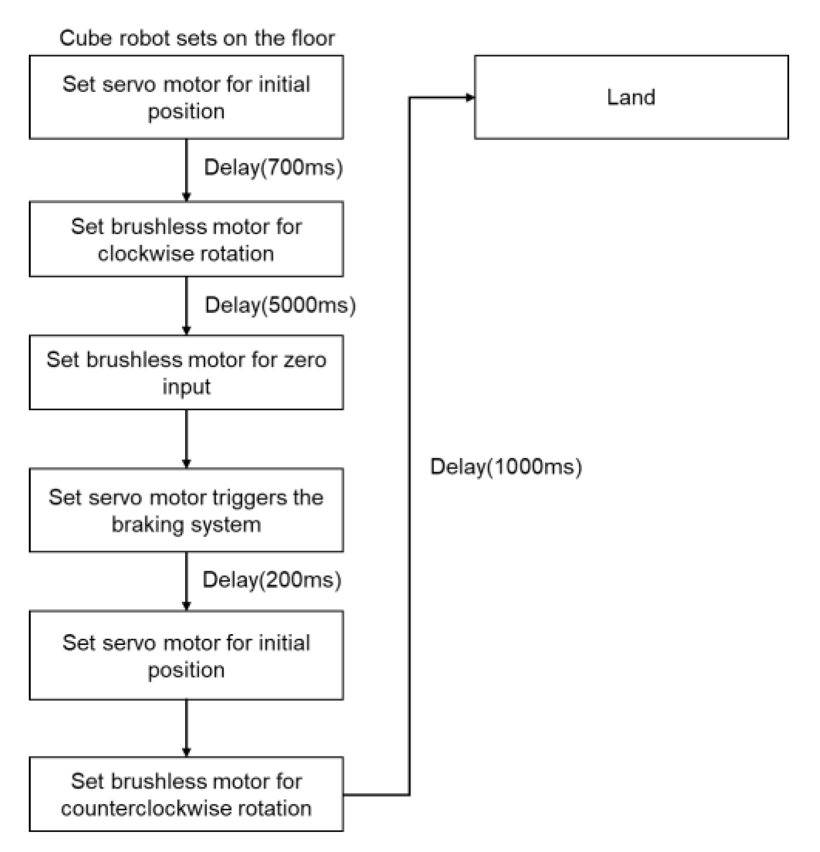
4.1. Bouncing Procedure

Figure 13 illustrates the bouncing procedure of the cube robot. First, the reaction wheel starts to rotate to generate enough kinetic energy. After saving enough energy, the brushless motor sets for zero input. Simultaneously, the servo motor triggers the braking system to stop the reaction wheel. During the bouncing, we set the brushless motor to rotate in a counterclockwise direction. Due to Newton’s Third Law, the same amount of torque made by the reaction wheel also applies to the cube robot in the opposite direction. Thus, it allows the cube robot to bounce up more easily.

4.2. Bouncing Up and Balancing Procedure

As shown in Figure 14, the cube robot’s procedure bouncing up and balancing can be divided into two parts: The left part is the main loop and the right part is the timer interrupt loop. The main loop is designed to be a while loop constantly checking whether the pitch angle of the cube robot is smaller than −39° (or bigger than 39°). The timer interrupt is designed to set the system to update the accelerations, the angular velocities, and the quaternion at every 5 ms. Once the pitch angle is smaller than −39°, which means the cube robot is lying on the horizontal floor, the reaction wheel will start rotating to generate the kinetic energy. The servo motor will trigger the braking system to collide with the reaction wheel after the reaction wheels rotates for 5 s. After the collision, once the cube robot has arrived near the equilibrium position (which is −6°~−39°), the parallel PID controller mentioned above will start its function for balancing the cube robot.

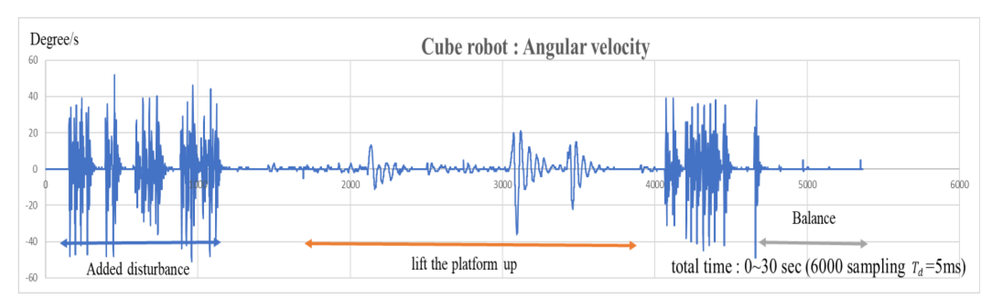
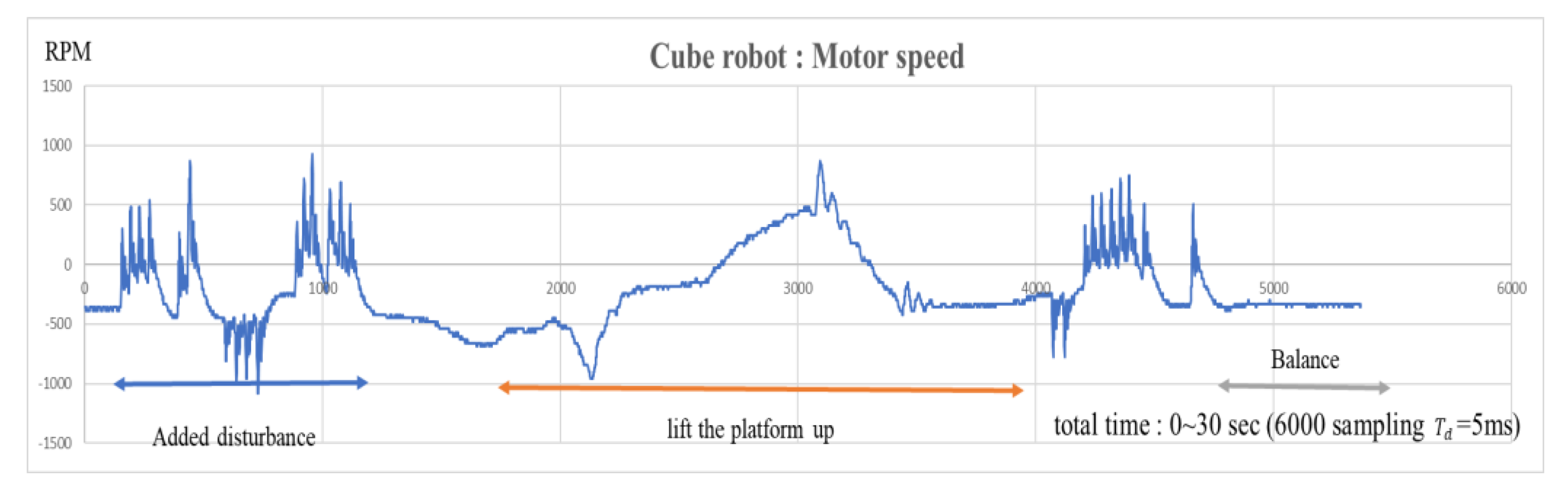
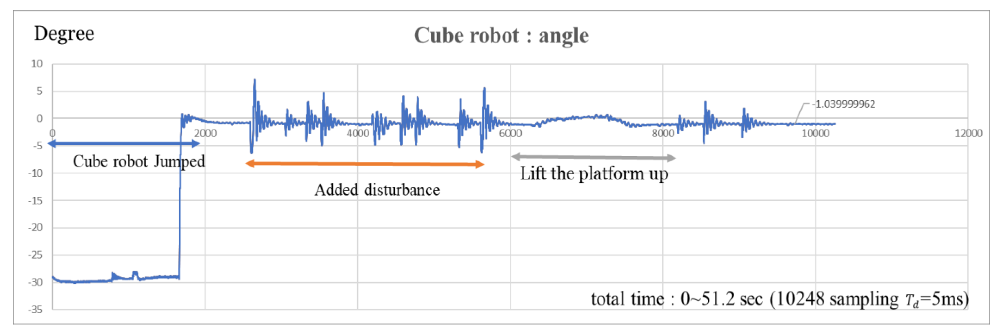
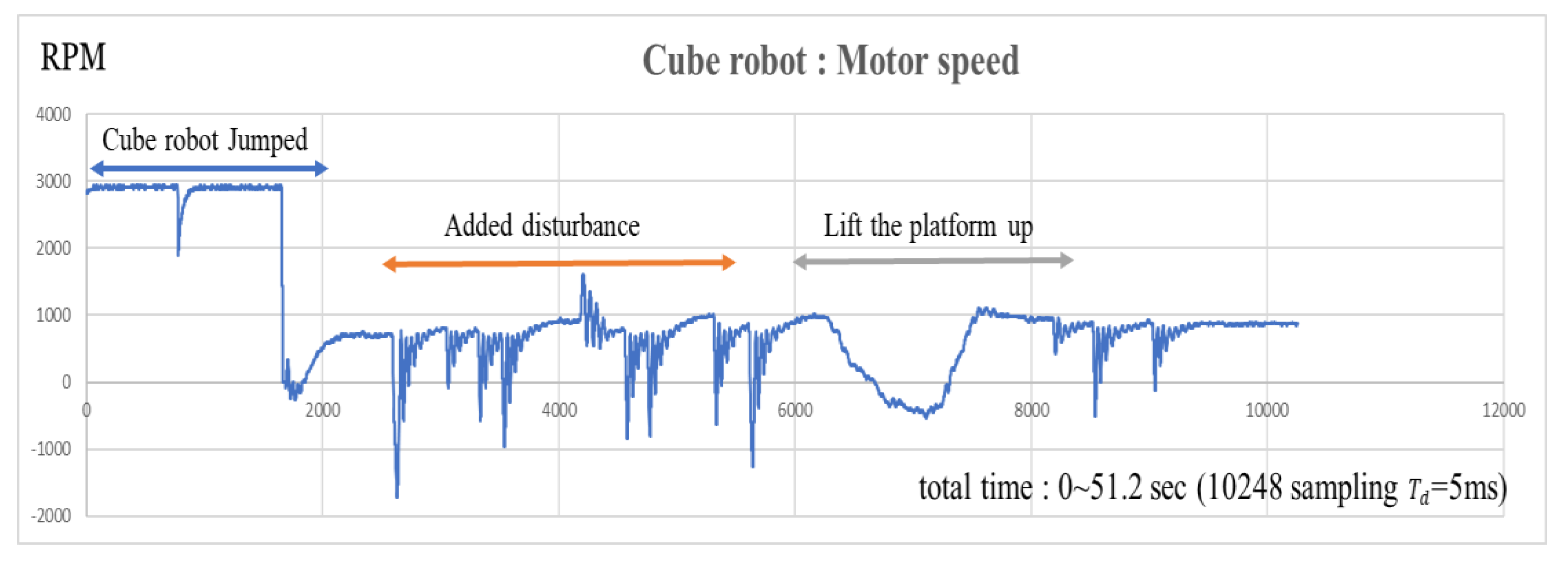
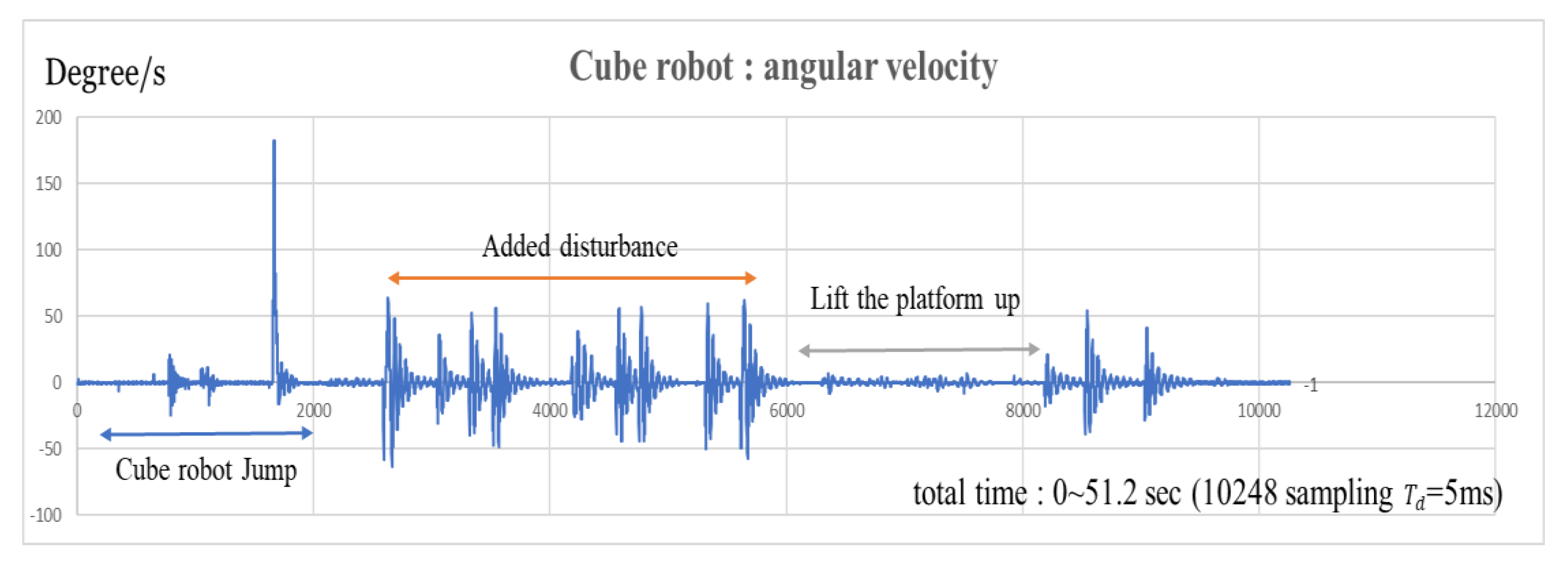
5. Experimental Results

To implement the discrete-time parallel PID controller, the sampling time $T_d$ of the system is set to be 5 ms. In the cube robot balancing, the input voltage is 20 V, and the PID parameters are given in Equation (20). The system’s robustness can be tested under two circumstances. The first additive disturbance is added to the cube robot to determine the extent of disturbance without changing balancing status. The second one is to lift the platform up to determine whether the cube can remain balanced at different inclination angles. Therefore, we used striking to generate external force disturbances, as shown in the provided video (see Supplementary Materials), to make the square robot deviate with 5.13 degrees, and then lift up and put down the platform to disturb the cube robot. After those disturbances, from Figure 15, Figure 16 and Figure 17, we can observe that the state variables $({\theta }_P,{\dot{\theta }}_P,{\dot{\theta }}_w)$ converge to (0.27°, 0(°/s), −330(rpm)). The experimental results reveal that after being disturbed by external disturbances, the cube robot can quickly return to the equilibrium position. In terms of the speed ${\dot{\theta }}_w$ of the inertia wheel, the motor will maintain a counterclockwise rotation during balance, about $-330(\mathrm{rpm})$. The reason is that the control algorithm used in this paper is the PID control method, and it cannot effectively save energy loss.

Next, we experiment with bouncing and balancing. As shown in Figure 18, the full bounce-up and balancing experiment starts with the rest at ${\theta }_P=-{30}^{°}$. As shown in Figure 19, the brushless motor accelerates the reaction wheel to 3000 rpm, and then the servo motor triggers the braking system to collide with the reaction wheel, allowing the cube robot to bounce up. Furthermore, from Figure 20, we observe that the angular velocity becomes rapidly high during the bounce. In this experiment, we also give external disturbances by striking the robot and lifting the platform. According to the measured state histories, the state variables $({\theta }_P,{\dot{\theta }}_P,{\dot{\theta }}_w)$ converge to (−1.03°, 0 (°/s), 870 (rpm)) and we can conclude that the cube robot can bounce and balance very robustly. We can find the equilibrium position is about $-{1.03}^{°}$ degrees. The overall center of gravity is slightly deviated from the center point due to the brake device.

6. Conclusions

This paper presented the mathematical modeling and realization of a cube robot with a PID balancing controller. The nonlinear dynamical model of the cube robot was derived and its controllability analyzed. A mechanical braking system was designed to convert the kinetic energy to potential energy and bounce up the robot. Furthermore, the attitude and heading reference system (AHRS) and parallel PID controller were proposed to balance the robot. The PID controller’s effectiveness was verified by the balance control experiment and robustness experiment, as demonstrated in the attached video (see Supplementary Materials). The PID controller could keep the cube robot balancing with good robustness performance. In future research, we will discuss improving the PID controller’s design so that its robustness and energy loss can be optimized.

References

1. Gajamohan, M.; Merz, M.; Thommen, I.; Andrea, R. The cubli: A cube that can jump up and balance. In Proceedings of the 2012 IEEE/RSJ International Conference on Intelligent Robots and Systems, Vilamoura, Algarve, Portugal, 7–12 October 2012; pp. 3722–3727. [Google Scholar]
2. Brian, D.O.; Moore, J.B. Optimal Control: Linear Quadratic Methods; Courier Corporation: North Chelmsford, MA, USA, 2007. [Google Scholar]
3. Chen, Z.; Ruan, X.; Li, Y.; Bai, Y.; Zhu, X. Dynamic modeling of a self-balancing cubical robot balancing on its edge. In Proceedings of the 2017 2nd International Conference on Robotics and Automation Engineering (ICRAE), Shanghai, China, 29–31 December 2017; pp. 11–15. [Google Scholar]
4. Chen, Z.; Ruan, X.; Li, Y.; Bai, Y.; Zhu, X. Dynamic modeling of a cubical robot balancing on its corner. In Proceedings of the MATEC Web of Conferences, Cheng Du, China, 16–17 December 2017; EDP Sciences: Paris, France, 2017; p. 0067. [Google Scholar]
5. Chen, Z.; Ruan, X.; Li, Y.; Zhu, X. A sliding mode control method for the cubical robot. In Proceedings of the 2018 13th World Congress on Intelligent Control and Automation (WCICA), Changsha, China, 4–8 July 2018; pp. 544–548. [Google Scholar]
6. Tian, L. Research on Fuzzy Control Algorithm of Cube System; Nanjing University of Science and Technology: Nanjing, China, 2006. [Google Scholar]
7. Muehlebach, M.; Dandera, R. Nonlinear analysis and control of a reaction-wheel-based 3-D inverted pendulum. IEEE Trans. Control Syst. Technol. 2017, 25, 235–246. [Google Scholar] [CrossRef]
8. Ang, K.; Chong, G.; Li, Y. PID control system analysis, design, and technology. IEEE Trans. Control Syst. Technol. 2005, 13, 559–576. [Google Scholar]
9. Nazaruddin, Y.Y.; Andrini, A.D.; Anditio, B. PSO Based PID Controller for Quadrotor with Virtual Sensor. IFAC Papers OnLine 2018, 51, 358–363. [Google Scholar] [CrossRef]
10. Fang, J.S.; Tsai, J.H.; Yan, J.J.; Tzou, C.H.; Guo, S.M. Design of Robust Trackers and Unknown Nonlinear Perturbation Estimators for a Class of Nonlinear Systems: HTRDNA Algorithm for Tracker Optimization. Mathematics 2019, 7, 1141. [Google Scholar] [CrossRef] [Green Version]
11. Li, Y.; Dempster, A.; Li, B.; Wang, J.; Rizos, C. A low-cost attitude heading reference system by combination of GPS and magnetometers and MEMS inertial sensors for mobile applications. J. Glob. Position. 2006, 5, 88–95. [Google Scholar] [CrossRef] [Green Version]
12. Che-Yu, L. Realization of One-Dimensional Cube Robot Capable of Bounce and Self-Balancing Based on Linear Quadratic Regulator Control. Master’s Thesis, Cheng Kung University, Tainan City, Taiwan, 2008. [Google Scholar]
13. Bar-itzhack, I.Y.; Oshman, Y. Attitude determination from vector observations: Quaternion estimation. IEEE Trans. Control Syst. Technol. 1985, 1, 128–136. [Google Scholar] [CrossRef]
14. Sheppred, S.W. Quaternion from rotation matrix. J. Guid. Control 1978, 1, 223–224. [Google Scholar] [CrossRef]
15. Krasjet. Quaternion and the Rotation in Three Dimensional; Department of Mathematics, Faculty of Science: Ankara, Turkey, 2018; pp. 24–35. [Google Scholar]
16. Zupan, E.; Saje, M.; Zupan, D. Quaternion-based dynamics of geometrically nonlinear spatial beams using the Runge–Kutta method. Finite Elem. Anal. Des. 2012, 54, 48–60. [Google Scholar] [CrossRef] [Green Version]
17. Farhangian, F.; Landry, R. Accuracy Improvement of Attitude Determination Systems Using EKF-Based Error Prediction Filter and PI Controller. Sensors 2020, 20, 4055. [Google Scholar] [CrossRef] [PubMed]
18. Zhi-Wei, W. Reduction of Vehicle Vibration and Energy Consumption on Rugged Roads by H∞ Control Laws. Master’s Thesis, National Chiao Tung University, Hsinchu City, Taiwan, 2003. [Google Scholar]
19. Bruton, S.L.; Kutz, J.N. Data-Driven Science and Engineering: Machine Learning, Dynamical Systems, and Control; Cambridge University Press: Cambridge, UK, 2019. [Google Scholar]
Figure 1. The prototype of the cube robot balancing on its edge.
Mathematics 08 01840 g001
Figure 2. The cube robot prototype.
Mathematics 08 01840 g002
Figure 3. The joint of the cube robot.
Mathematics 08 01840 g003
Figure 4. The torque and rotation angle of the cube robot.
Mathematics 08 01840 g004
Figure 5. The torque of the reaction wheel.
Mathematics 08 01840 g005
Figure 6. The gadget of the braking system.
Mathematics 08 01840 g006
Figure 7. The server motor of the braking system.
Mathematics 08 01840 g007
Figure 8. The braking system.
Mathematics 08 01840 g008
Figure 9. The signal processing units of the cube robot.
Mathematics 08 01840 g009
Figure 10. The schematic diagram of the attitude and heading reference system (AHRS).
Mathematics 08 01840 g010
Figure 11. The structure of the cube robot balancing control.
Mathematics 08 01840 g011
Figure 12. The process of the cube robot bouncing control.
Mathematics 08 01840 g012
Figure 13. The flow chart of the cube robot bouncing control.
Mathematics 08 01840 g013
Figure 14. The flow chart of bounce and balance control.
Mathematics 08 01840 g014
Figure 15. Time response of the tilt angle θ P of the cube robot balancing on its edge.
Mathematics 08 01840 g015
Figure 16. Time response of the tilt angle angular velocity θ ˙ P of the cube robot balancing on its edge.
Mathematics 08 01840 g016
Figure 17. Time response of the motor speed θ ˙ w of the cube robot balancing on its edge.
Mathematics 08 01840 g017
Figure 18. Time response of the tilt angle θ P of the cube robot bouncing and balancing on its edge.
Mathematics 08 01840 g018
Figure 19. Time response of the motor speed θ ˙ w of the cube robot bouncing and balancing on its edge.
Mathematics 08 01840 g019
Figure 20. Time response of the tilt angle angular velocity θ ˙ P of the cube robot bouncing and balancing on its edge.
Mathematics 08 01840 g020