Individual Variability in Dispersal and Invasion Speed

Abstract

We model the growth, dispersal and mutation of two phenotypes of a species using reaction–diffusion equations, focusing on the biologically realistic case of small mutation rates. Having verified that the addition of a small linear mutation term to a Lotka–Volterra system limits it to only two steady states in the case of weak competition, an unstable extinction state and a stable coexistence state, we exploit the fact that the spreading speed of the system is known to be linearly determinate to show that the spreading speed is a nonincreasing function of the mutation rate, so that greater mixing between phenotypes leads to slower propagation. We also find the ratio at which the phenotypes occur at the leading edge in the limit of vanishing mutation.

1. Introduction

The speed at which a species expands its range is a fundamental parameter in ecology, evolution and conservation biology. Knowledge of this speed enables us to predict the ability of a species to keep up with the rate at which the climate changes or the rate at which an exotic species invades, representing two prominent ecological challenges [1,2]. It is known that traits such as dispersal and population growth affect the rate at which a species expands its range, and there has been a suggestion in recent work that polymorphism in traits could cause a species invasion to occur at a faster rate than a single morph would in isolation [3,4]. Understanding the effect that each trait of a species has, and could potentially have, on its rate of spread is therefore important to understanding how the spread of a species can evolve.

Most common models of invasions in population dynamics incorporate aspects of dispersal and growth, e.g., works by the authors of [5,6,7,8], however the mutation of one phenotype to another has been a less common inclusion. Even the addition of a simple mutation term can dramatically affect the behaviour of a model. A review of Cosner [9] singles out two models that involve mutation and multiple dispersal strategies in a population of a species: the model introduced in Elliott and Cornell [3] to investigate dispersal polymorphism for two morphs, in which a simple linear mutation is used, and the model of Bouin et al. [10], motivated by the destructive invasion of cane toads across northern Australia, in which mutations are considered to act as a diffusion process in the phenotype space.

Elliott and Cornell assume that the spread rate of the two phenotypes in their system, usually referred to as the spreading speed, is determined by the linearisation of their system at the extinction state zero. This assumption can be rigorously proved to hold under reasonable conditions on the parameters; see the framework of Girardin [11], which applies in particular to this model, and also, for an alternative approach, Morris [12], where the assumption is proved using earlier results of Wang [13] in the case where the mutation rate is small, which is generally the case for all organisms since natural selection typically acts to minimize mutation rate [14]. Moreover, in addition to being linearly determined, the spreading speed equals the minimal speed of a class of travelling waves [11,12], mimicking well-known results on travelling waves and spreading speeds for the Fisher–KPP equation [15,16,17].

Knowing that the rate of spread is linearly determinate and linked to travelling wave speeds provides a powerful tool that we exploit here to deduce ecologically-important information about the invasion of trait-structured species using the model introduced in [3]. In particular, we establish results on the dependence of spreading speeds on the mutation rate, and on the composition of the leading edge of minimal speed travelling waves in the limit of vanishing mutation. Some of our results focus, as in [3], on the case when different morphs have varying dispersal abilities or strategies, and in addition, there is a trade-off between dispersal and growth. Such trade-offs are exhibited by many species, including certain plants, insects and terrestrial arthropods; see, for instance, the review of Bonte et al. [18] on the costs of dispersal.

Elliott and Cornell’s model examines the interaction between an establisher phenotype with population density $n_e$, and a disperser phenotype with population density $n_d$, using a Lotka–Volterra competition system:

$$\begin{array}{cc}\hfill \frac{\partial n_e}{\partial t}& =D_e\frac{{\partial }^2{n}_e}{\partial x^2}+r_e{n}_e(1-m_{ee}{n}_e-m_{ed}{n}_d)-\mu e{n}_e+\mu d{n}_d\hfill \\ \hfill \frac{\partial n_d}{\partial t}& =D_d\frac{{\partial }^2{n}_d}{\partial x^2}+r_d{n}_d(1-m_{de}{n}_e-m_{dd}{n}_d)-\mu d{n}_d+\mu e{n}_e.\hfill \end{array}$$

(1)

The first term on the right hand side of each equation represents the dispersal of the phenotype through diffusion, where $D_e$ and $D_d$ are the dispersal rates of each morph. The second term describes the growth rate of the phenotype using a logistic term, this is similar to what is used in Fisher’s model [16]. We use $r_e$ and $r_d$ to represent the growth rate of each morph, $m_{ee}$ and $m_{dd}$ represent the intramorph competition, while $m_{ed}$ and $m_{de}$ represent the intermorph competition. The third and fourth terms represent a linear mutation between the phenotypes at mutation rates of $\mu e$ and $\mu d$, where $\mu$, e and d are constants. Note that we slightly modify the model in the work by the authors of [3] here by replacing the parameters ${\mu }_e,{\mu }_d$ in the work by the authors of [3] with $\mu e$ and $\mu d$ to enable dependence on mutation to be investigated by variation of the single parameter $\mu$. It is assumed that all parameters of the system are positive real numbers.

As in the work by the authors of [3], we suppose a basic trade-off between dispersal and growth, namely, that the establisher phenotype has the larger growth rate, while the disperser phenotype has the larger dispersal rate,

$$r_e>r_d,D_d>D_e.$$

(2)

While trade-off (2) is not needed either in the proof of linear determinacy or in some of our results on the dependence of spreading speed on mutation rate, we will make use of (2) to discuss parameter-dependent options for the vanishing-mutation limit of spreading speeds in Section 3, and in Section 4, where we characterize the composition of the leading edge of solutions of (1). Further discussion on interesting possible implications of dispersal–growth trade-offs for this model is presented in [12]. Following classical competition theory [19], we suppose throughout that the intramorph competition is greater than the intermorph competition,

$$m_{dd}>m_{ed},m_{ee}>m_{de}.$$

(3)

We also have in mind throughout that the mutation rate $\mu$ is relatively small in comparison to the other parameters, to remain biologically realistic [14].

Kolmogorov, Petrovskii and Piskunov [15] studied the existence of monotonic travelling wave solutions of the scalar form of the equation

$$\frac{\partial u}{\partial t}=A\frac{{\partial }^{2}u}{\partial x^2}+f\left(u\right).$$

(4)

Throughout this work, we will consider travelling wave solutions to be solutions of the Equation (4) of the form $u(x,t)=w(x-ct)$, where $w:{\mathbb{R}}^n\to {\mathbb{R}}^n$ is called the wave profile and $c\in \mathbb{R}$ is the speed of the wave. Kolmogorov, Petrovskii and Piskunov studied the case when $n=1$, $A=d$ and $f\left(u\right)=ru(1-u)$, proposed by Fisher [16], and proved there is a continuum of values of c for which a monotonic travelling wave solution exists, specifically if $c\ge c^{*}$, where $c^{*}=2\sqrt{rd}$ is the minimal travelling wave speed, as well as establishing stability properties of the minimal-speed front. Aronson and Weinberger [17] further studied this system and characterised $c^{*}$ as a spreading speed. These results were extended to cooperative systems of equations for a suitable class of nonlinearities f by Volpert, Volpert and Volpert [20].

The system (1) is of the form (4) if we let $u={(n_e,n_d)}^T\in {\mathbb{R}}^2$, A be a diagonal matrix containing the dispersal rates,

$$A=\left(\begin{array}{cc}{D}_e& 0\\ 0& D_d\end{array}\right),$$

(5)

and f be a nonlinear function containing the growth, competition and mutation terms,

$$f(n_e,n_d)=\left(\begin{array}{c}{r}_e{n}_e(1-m_{ee}{n}_e-m_{ed}{n}_d)-\mu e{n}_e+\mu d{n}_d\\ r_d{n}_d(1-m_{de}{n}_e-m_{dd}{n}_d)+\mu e{n}_e-\mu d{n}_d\end{array}\right).$$

(6)

In the following, we will use the notation $u>v$ to denote that the ith component of each vector satisfies $u_i>v_i$, for each i, similarly for $u<v$, $u\ge v$ and $u\le v$. We say that $u\in {\mathbb{R}}^n$ is positive if $u>0$. The notation $u\in (a,b]$ denotes that the ith component of each vector satisfies the inequality $a_i<u_i\le b_i$ for each i.

Elliott and Cornell investigated numerically the effect of varying the parameters on the spreading speed of the system and interestingly found that, for certain values of growth and dispersal rate, the system would spread faster in the presence of both phenotypes than just one phenotype would spread in the absence of mutation [3]. They predict the spreading speed obtained for each set of parameters in the limit of small mutation, using the front propagation method of van Saarloos [21], making the assumption that the spreading speed of system (1) is linearly determinate in order to do so. As $\mu \to 0$ the three possible limiting speeds are

$$v_e=2\sqrt{r_e{D}_e},v_d=2\sqrt{r_d{D}_d},v_f=\frac{|r_e{D}_d-r_d{D}_e|}{\sqrt{(r_e-r_d)(D_d-D_e)}}.$$

(7)

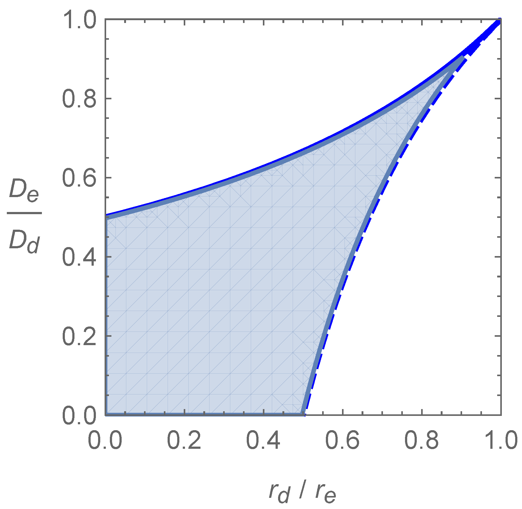
Condition (2) is enough to ensure that $v_f$ exists and is faster than $v_e$ and $v_d$, which are the spreading speeds of the two Fisher–KPP equations that would be satisfied by each phenotype in isolation. The faster speed $v_f$ is predicted for parameters in the region of the positive quadrant of $\left(r_d/r_e,D_e/D_d\right)$-space, which satisfies the inequalities

$$\frac{D_d}{D_e}+\frac{r_d}{r_e}>2,\frac{D_e}{D_d}+\frac{r_e}{r_d}>2,$$

(8)

represented by the shaded area in Figure 1.

The spreading speed of the system is said to be linearly determinate if it is the same as the spreading speed of the system obtained when (1) is linearised about the $(0,0)$ equilibrium, namely,

$$\begin{array}{cc}\hfill \frac{\partial n_e}{\partial t}& =D_e\frac{{\partial }^2{n}_e}{\partial x^2}+(r_e-\mu e)n_e+\mu d{n}_d\hfill \\ \hfill \frac{\partial n_d}{\partial t}& =D_d\frac{{\partial }^2{n}_d}{\partial x^2}+(r_d-\mu d)n_d+\mu e{n}_e.\hfill \end{array}$$

(9)

This assumption is one that is suggested by the numerical studies in [3], but is not always true even in the scalar case [21,22,23,24]. Stokes [25] calls the minimal wave speed $c^{*}$ “pulled” if it is equal to the linearised spreading speed, that is, the speed of the front is determined by the individuals at the leading edge. Similarly the minimal wave speed is said to be “pushed” if its speed is greater than the linearised spreading speed, in this case the speed is determined by individuals behind the leading edge. Typically there are qualitative differences in wave behaviour depending on whether the wave is pushed or pulled, e.g., stability in the scalar case is discussed in the work by the authors of [26].

In the case of systems, most sufficient conditions for linear determinacy require a cooperative assumption on the system. A system is cooperative when the off-diagonal elements of the Jacobian matrix of f are always non-negative, i.e.,

$$\frac{\partial f_i\left(u\right)}{\partial u_j}\ge 0,\mathrm{if}i\ne j.$$

(10)

In biological terms this would mean that each phenotype benefits from the presence of others. A cooperative system is useful mainly due to the existence of a comparison principle for such systems [27,28], which is useful in particular in the proof of linear determinacy.

Theorem 1

(Comparison Principle [13], Theorem 3.1). Let A be a positive definite diagonal matrix. Assume that f is a vector-valued function in ${\mathbb{R}}^n$ that is continuous and piecewise continuously differentiable in $\mathbb{R}$, and that the underlying system (4) is cooperative. Suppose that $u(x,t)$ and $v(x,t)$ are bounded on $\mathbb{R}\times [0,\infty )$ and satisfy

$$\frac{\partial u}{\partial t}-A\frac{{\partial }^{2}u}{\partial x^2}-f\left(u\right)\le \frac{\partial v}{\partial t}-A\frac{{\partial }^{2}v}{\partial x^2}-f\left(v\right)$$

If $u(x,t_0)\le v(x,t_0)$ for $x\in \mathbb{R}$, then

$$u(x,t)\le v(x,t),\mathrm{for}x\in \mathbb{R},t\ge t_0.$$

Linear determinacy was shown to hold for some cooperative systems by Lui [27], and the result was extended to more general cooperative systems by Weinberger, Lewis and Li [28], who assumed, in particular, that for any positive eigenvector q of $f^{\prime }\left(0\right)$,

$$f\left(\alpha q\right)\le \alpha f^{\prime }\left(0\right)q,\mathrm{for}\alpha >0.$$

(11)

This reduces to a condition imposed by Hadeler and Rothe [23] in the scalar case.

Unfortunately, we see from the Jacobian matrix (12) that our system (1) is only partially cooperative,

$$J_f(n_e,n_d)=\left(\begin{array}{cc}{r}_e(1-2m_{ee}{n}_e-m_{ed}{n}_d)-\mu e& \mu d-r_e{m}_{ed}{n}_e\\ \mu e-r_d{m}_{de}{n}_d& r_d(1-m_{de}{n}_e-2m_{dd}{n}_d)-\mu d\end{array}\right).$$

(12)

In fact it is typically only cooperative at small population densities due to the relative smallness of the mutation term (see Figure 2).

However, Girardin [11] has recently established a linear determinacy result for a class of non-cooperative reaction–diffusion systems that includes the case considered here; see Theorem 1.7, together with Theorems 1.5 and 1.6, of Girardin [11], which apply here because when $(n_e,n_d)=(0,0)$, the Jacobian (12) always has at least one positive eigenvalue, which can be seen from arguments similar to those used in the proof of Proposition 3.1 below. An alternative proof of linear determinacy for the particular system (1) is given by Morris [12], Theorems 4.5 and 2.15, using the linear determinacy framework outlined by Wang [13]. This latter result is proved under the assumption of sufficiently small mutation and intermorph competition, and uses the fact that (1) is cooperative at low population densities to trap the nonlinearity f between two cooperative nonlinearities, $f^{-}$ and $f^{+}$.

Exploiting this linear determinacy, we answer ecologically important questions pertaining to our system in the case of small mutation rate. We first take advantage of a Perron–Frobenius structure to investigate the effect of mutation on spreading speed, and show that an increase in mutation between morphs results in a decrease in the value of the spreading speed; see Theorem 3. This slowing of the speed of propagation as the mutation rate increases is mathematically related, in fact, to the so-called ‘reduction phenomenon’, that greater mixing lowers growth, discussed in Altenberg [29]. Secondly we investigate the composition of the leading edge of invasion in the limit of small mutation rate, and demonstrate the effects of dispersal, growth rate and mutation on this composition. As a by-product, we also characterise the vanishing-mutation limit of the spreading speed for three different regimes of diffusion and growth parameters in Theorem 2, which yields, in particular, a rigorous explanation of the parameter-dependent selection criteria for the three possible limiting speeds (7) that were discussed in the work by the authors of [3].

We draw the reader’s attention to two further interesting references that tackle questions for systems related to (1). Griette and Raoul [30], motivated by an epidemiological model, studied the existence and properties of travelling waves for a special case of system (1). They assume, in particular, that $D_e=D_d$, of which advantage can be taken to prove an explicit formula for the spreading speed and to characterise the shape of travelling wave solutions, including proving non-monotone behaviour in one phenotype and asymptotic behaviour at $\pm \infty$. Clearly this assumption of equal dispersal rates, though realistic for the modelling of wild type and mutant types of a virus in the work by the authors of [30] and extremely useful mathematically, is not reasonable for the dispersal polymorphism that is our focus here. Cantrell, Cosner and Yu [31] study (1) from the perspective not of propagation phenomena but of dynamics on a bounded domain. They provide a detailed study of equilibria, the phase plane and dynamics for a range of different parameters, including various regimes for the competition parameters $m_{ee},m_{ed},m_{ed},m_{de}$.

The rest of the paper is organised as follows. Section 2 presents preliminary material on equilibria of the system (1) and their relationship to equilibria for the related competition–diffusion system when $\mu =0$. The effect of mutation on spreading speeds is discussed in Section 3, using the characterisation of the spreading speed as the linearly-determined minimal speed of a family of travelling waves, which can be expressed and analysed in terms of Perron–Frobenius matrix theory. Section 4 focusses on the parameter regime, in which the dispersal and growth of both morphs play a role in the vanishing-mutation limit of the spreading speed and derives an expression for the ratio of the morphs in the leading edge of the invasion in this case. Some conclusions and remarks are given in Section 5.

2. Equilibria of the System

We begin with a brief discussion of the equilibria of the system (1) under our assumption (3) on the competition parameters; see also the work by the authors of [31] for further investigation of equilibria of (1). A much studied competition–diffusion system, similar to (1) but where there is no mutation between phenotypes and both intramorph competition values equal one, is the Lotka–Volterra system of equations [32,33,34,35],

$$\begin{array}{cc}\hfill \frac{\partial n_e}{\partial t}& =D_e\frac{{\partial }^2{n}_e}{\partial x^2}+r_e{n}_e(1-n_e-m_{ed}{n}_d),\hfill \\ \hfill \frac{\partial n_d}{\partial t}& =D_d\frac{{\partial }^2{n}_d}{\partial x^2}+r_d{n}_d(1-n_d-m_{de}{n}_e).\hfill \end{array}$$

(13)

Lewis, Li and Weinberger [5] note that a coexistence equilibrium for this system (13) exists if, and only if, $(1-m_{ed})(1-m_{de})>0$; that is, either when both $m_{ed}<1$ and $m_{de}<1$, or both $m_{ed}>1$ and $m_{de}>1$. Note that the case where $m_{ed}<1$ and $m_{de}<1$ corresponds to the condition (3) in our system (1). A stability analysis shows that this coexistence equilibrium is stable when $m_{ed}<1$ and $m_{de}<1$, and unstable when $m_{ed}>1$ and $m_{de}>1$, where here stability is understood in the sense of stability of the ODE system given by (13) with $D_e=D_d=0$. It should also be noted that the works by the authors of [5,34] also study the case where one species invades the territory of another, while we, and also the authors of [3,30], are concerned with two morphs of a species invading a previously unoccupied territory.

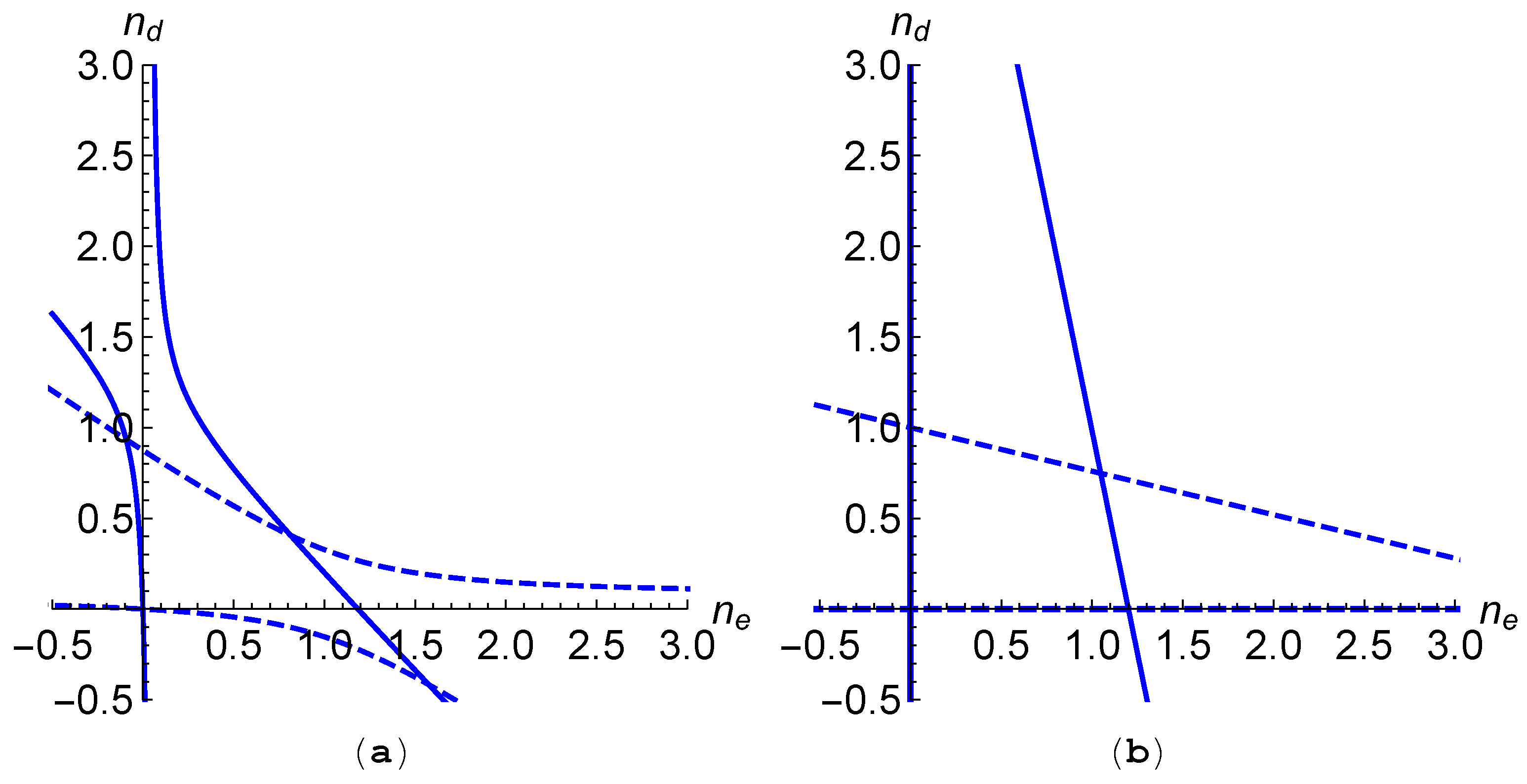
For our system (1) we can easily see that there only exist two constant equilibria by plotting the nullclines of (6),

$$\begin{array}{cc}\hfill r_e{n}_e(1-m_{ee}{n}_e-m_{ed}{n}_d)-\mu e{n}_e+\mu d{n}_d& =0,\hfill \end{array}$$

(14)

$$\begin{array}{cc}\hfill r_d{n}_d(1-m_{de}{n}_e-m_{dd}{n}_d)-\mu d{n}_d+\mu e{n}_e& =0,\hfill \end{array}$$

(15)

and observe where they intersect. The nullclines confirm for a specific choice of parameters that we only have two non-negative equilibria and that they are the extinction equilibrium and a single coexistence equilibrium (Figure 3a). The nullclines appear as they do in Figure 3a if the parameters satisfy the conditions

$$\frac{\mu d}{r_e{m}_{ed}}<\frac{r_e-\mu e}{r_e{m}_{ee}},\frac{\mu e}{r_d{m}_{de}}<\frac{r_d-\mu d}{r_d{m}_{dd}},$$

(16)

which aligns with our assumption that the mutation is relatively small. We note that it is clearly also possible to deal with cases in which the mutation does not satisfy assumptions (16), however we are only interested in the case of small mutation here.

However, simply plotting the nullclines of our system does not tell us the stability of each equilibrium, we therefore consider a modified version of (6) without the mutation terms, which we call g,

$$g(n_e,n_d)=\left(\begin{array}{c}{r}_e{n}_e(1-m_{ee}{n}_e-m_{ed}{n}_d)\\ r_d{n}_d(1-m_{de}{n}_e-m_{dd}{n}_d)\end{array}\right).$$

(17)

Due to the relative smallness of the mutation terms, we can then introduce them as a perturbation before using the implicit function theorem.

First we evaluate the equilibria of g. We can easily see that there are four equilibria by plotting the nullclines,

$$\begin{array}{cc}\hfill r_e{n}_e(1-m_{ee}{n}_e-m_{ed}{n}_d)& =0,\hfill \end{array}$$

(18)

$$\begin{array}{cc}\hfill r_d{n}_d(1-m_{de}{n}_e-m_{dd}{n}_d)& =0,\hfill \end{array}$$

(19)

which we do in Figure 3b for certain parameters. The equilibria of (17) consist of an extinction equilibrium $(0,0)$, two equilibria on the axes where one phenotype is present while the other is extinct, $\left(1/m_{ee},0\right)$, $\left(0,1/m_{dd}\right)$, and a coexistence equilibrium

$$\left({\displaystyle \frac{m_{dd}-m_{ed}}{m_{ee}{m}_{dd}-m_{ed}{m}_{de}}},{\displaystyle \frac{m_{ee}-m_{de}}{m_{ee}{m}_{dd}-m_{ed}{m}_{de}}}\right)$$

which we refer to as $(n_e^{*},n_d^{*})$ for simplicity. Note that $(n_e^{*},n_d^{*})$ is a coexistence equilibria due to the condition (3) specified earlier.

The Jacobian of (17) is

$$J_g(n_e,n_d)=\left(\begin{array}{cc}{r}_e(1-2m_{ee}{n}_e-m_{ed}{n}_d)& -r_e{m}_{ed}{n}_e\\ -r_d{m}_{de}{n}_d& r_d(1-m_{de}{n}_e-2m_{dd}{n}_d)\end{array}\right).$$

(20)

Substituting in values of $n_e$ and $n_d$ at each of the equilibria to the trace and determinant of (20) we see that the equilibrium $(n_e^{*},n_d^{*})$ is stable, while the other three are unstable. Note also that the determinant of (20) is non-zero when evaluated at each of the equilibria of (17).

We now use the implicit function theorem [36] to determine how each equilibrium moves when mutation is introduced to the system (17) as a perturbation. To do so, we suppose that there exists $\mu >0$ such that

$$f(n_e,n_d)=g(n_e,n_d)+\mu M\left(\begin{array}{c}{n}_e\\ n_d\end{array}\right)$$

(21)

where g is defined in (17) above, $\mu$ is a non-negative scalar parameter which we use to vary the mutation and M is the matrix of mutation coefficients

$$M=\left(\begin{array}{cc}-e& d\\ e& -d\end{array}\right).$$

(22)

The equilibria for our original system (1) satisfy $f(n_e,n_d)=0$, where f is the nonlinearity (6), so that

$$g(n_e,n_d)+\mu M\left(\begin{array}{c}{n}_e\\ n_d\end{array}\right)=0.$$

(23)

As a consequence of the implicit function theorem, in a neighbourhood of $\mu =0$ and an equilibrium $({\overline{n}}_e,{\overline{n}}_d)$ of g, there is a unique solution of (23) which is a continuously differentiable function of $\mu$, say $h_{({\overline{n}}_e,{\overline{n}}_d)}\left(\mu \right)$, provided g is invertible at $({\overline{n}}_e,{\overline{n}}_d)$. This ensures we can differentiate (23) in order to obtain an expression describing how an equilibrium ${({\overline{n}}_e,{\overline{n}}_d)}^T$ is perturbed upon the introduction of mutation $\mu$. Since the determinant of the Jacobian matrix $J_g$ is not equal to zero at any of the equilibria, we may invert $J_g$ and obtain the expression

$$\mathsf{\Theta }({\overline{n}}_e,{\overline{n}}_d):=\frac{\mathrm{d}}{\mathrm{d}\mu }{h}_{({\overline{n}}_e,{\overline{n}}_d)}\left(\mu \right){|}_{\mu =0}=-J_g{({\overline{n}}_e,{\overline{n}}_d)}^{-1}M\left(\begin{array}{c}{\overline{n}}_e\\ {\overline{n}}_d\end{array}\right).$$

(24)

Clearly the extinction equilibrium $(0,0)$ remains at $(0,0)$, and the implicit function theorem ensures the local uniqueness of this equilibrium for small $\mu >0$. Evaluating (24) at each of the other equilibria of g, we see that the equilibrium $\left(1/m_{ee},0\right)$ is perturbed into the lower right quadrant, because

$$\mathsf{\Theta }\left(\frac{1}{m_{ee}},0\right)=\frac{\mu e}{r_e{r}_d(m_{ee}-m_{de})}{\left(\frac{r_e{m}_{ed}}{m_{ee}}-\frac{r_d}{m_{ee}}(m_{ee}-m_{de}),-r_e\right)}^T.$$

(25)

Note that the term $(m_{ee}-m_{de})$ is positive due to the condition (3). Similarly, the equilibrium $\left(0,1/m_{dd}\right)$ is perturbed into the upper left quadrant, since

$$\mathsf{\Theta }\left(0,\frac{1}{m_{dd}}\right)=\frac{\mu d}{r_e{r}_d(m_{dd}-m_{ed})}{\left(-r_d,\frac{r_d{m}_{de}}{m_{dd}}-\frac{r_e}{m_{dd}}(m_{dd}-m_{ed})\right)}^T.$$

(26)

Finally, the coexistence equilibrium is perturbed a small amount in a direction which is dependant on the parameters of the system,

$$\mathsf{\Theta }\left(n_e^{*},n_d^{*}\right)=\left(\begin{array}{c}{r}_e{n}_e^{*}{n}_d^{*}\left[\mu e(m_{dd}-m_{ed})-\mu d(m_{ee}-m_{de})\right]\\ r_d{n}_e^{*}{n}_d^{*}\left[\mu d(m_{ee}-m_{dd})-\mu e(m_{dd}-m_{ed})\right]\end{array}\right).$$

(27)

Moreover, since the Jacobian is a continuous function of $\mu$, we know that for small $\mu \ne 0$, the stability of each of the equilibria remains the same as when $\mu =0$. Therefore, by introducing a small amount of mutation to our system, we are left with two non-negative equilibria: an unstable extinction state $(0,0)$ and a stable coexistence state $(n_e^{*},n_d^{*})$.

3. The Role of Mutation in Spreading Speeds

In this and the following section, we derive predictions about the spreading of species modelled by (1) by exploiting the linear determinacy of the system together with the fact that the spreading speed can be characterised using travelling waves.

We being by deriving a $\mu$-dependent expression for the minimal travelling wave speed of the linearisation of (1) about the origin. If the general reaction–diffusion system (4) admits a travelling wave solution $u(x,t)=w(x-ct)$, then by substituting $w(x-ct)$ in to the general form (4) we may write the system in the form of a travelling wave equation:

$$A{w}^{″}\left(\xi \right)+c{w}^{\prime }\left(\xi \right)+g\left(w\left(\xi \right)\right)+\mu Mw\left(\xi \right)=0.$$

(28)

We now have an ordinary differential equation in the single variable $\xi =x-ct$, the linearisation of which about the origin is

$$A{w}^{″}\left(\xi \right)+c{w}^{\prime }\left(\xi \right)+g^{\prime }\left(0\right)w\left(\xi \right)+\mu Mw\left(\xi \right)=0.$$

(29)

Further, if we substitute the ansatz solution $w\left(\xi \right)=e^{-\beta \xi }q$ into (29), we obtain the eigenvalue problem

$$\left(\beta A+{\beta }^{-1}(g^{\prime }\left(0\right)+\mu M)\right)q=cq,$$

(30)

where $\beta >0$ is the spatial decay and $q>0$ denotes the phenotypic distribution at the leading edge. We define the matrix on the left hand side to be

$$H_{\beta ,\mu }:=\beta A+{\beta }^{-1}(g^{\prime }\left(0\right)+\mu M)=\beta A+{\beta }^{-1}{f}^{\prime }\left(0\right).$$

(31)

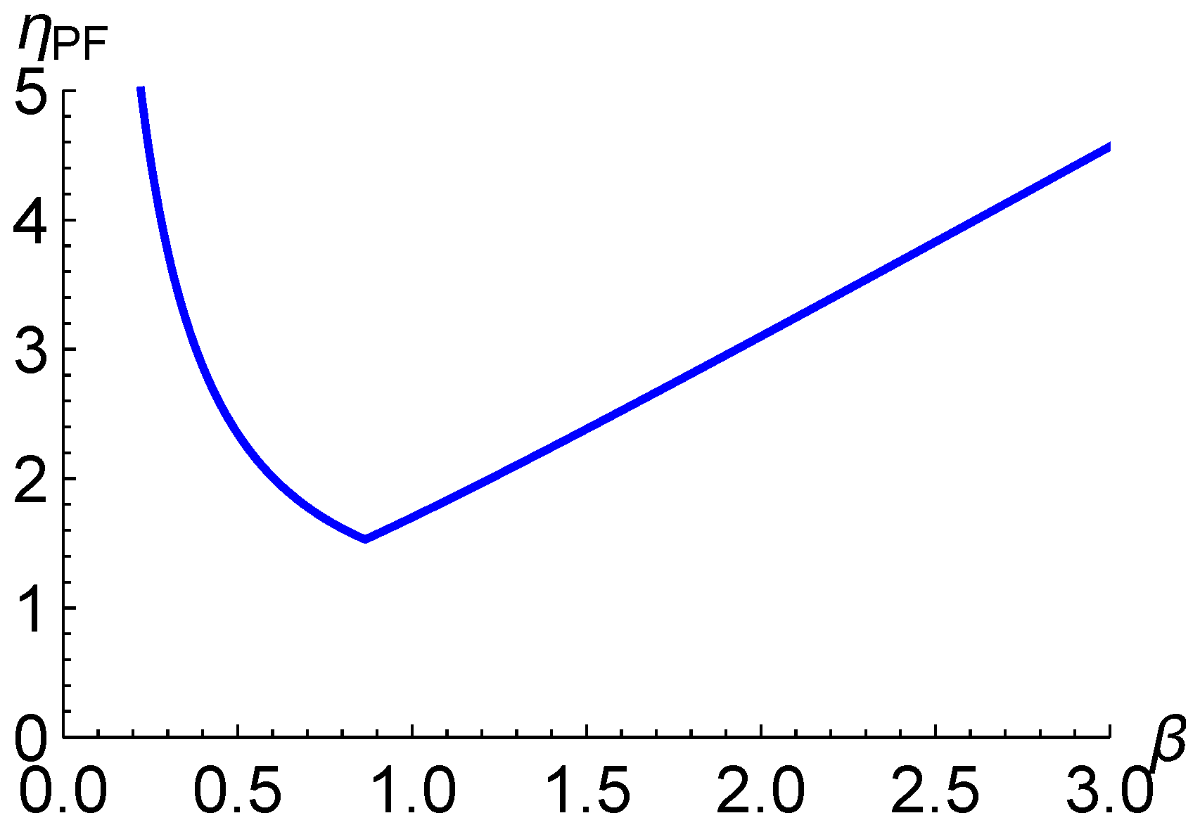
For $\mu >0$ the matrix $H_{\beta ,\mu }$ has strictly positive off-diagonal elements and therefore by the Perron–Frobenius theorem has a Perron–Frobenius eigenvalue, which is plotted in Figure 4 as a function of $\beta$. This Perron–Frobenius eigenvalue, which we denote ${\eta }_{\mathrm{PF}}\left(H_{\beta ,\mu }\right)$, is the larger of the two real eigenvalues of $H_{\beta ,\mu }$ and has a one-dimensional eigenspace spanned by a positive eigenvector. Further, this Perron–Frobenius eigenvalue is positive for every $\beta ,\mu >0$.

Proposition 1.

The Perron–Frobenius eigenvalue of the matrix $\beta A+{\beta }^{-1}{f}^{\prime }\left(0\right)$ is strictly positive for all $\mu >0$, $\beta >0$

Proof. 

Multiplying the matrix $\beta A+{\beta }^{-1}{f}^{\prime }\left(0\right)$ on the right by ${(d,e)}^T$ we obtain

$$(\beta A+{\beta }^{-1}{f}^{\prime }\left(0\right))\left(\begin{array}{c}d\\ e\end{array}\right)=\left(\begin{array}{c}\beta D_{e}d+{\beta }^{-1}{r}_{e}d\\ \beta D_{d}e+{\beta }^{-1}{r}_{d}e\end{array}\right)>0.$$

(32)

By Corollary 1.6 of Crooks [37], this implies

$${\eta }_{\mathrm{PF}}(\beta A+{\beta }^{-1}{f}^{\prime }\left(0\right))>0.$$

(33)

 □

Definition 1.

The minimal speed of the travelling wave solution$w\left(\xi \right)=e^{-\beta \xi }q$of (28) for a given $\mu >0$ is given by

$$\eta \left(\mu \right):=\underset{\beta >0}{inf}{\eta }_{\mathrm{PF}}\left(H_{\beta ,\mu }\right).$$

(34)

We define $\beta \left(\mu \right)$ to be the value of β at which $\eta \left(\mu \right)$ is attained.

Note that it follows from Gershgorin’s Circle Theorem that ${\eta }_{\mathrm{PF}}\left(H_{\beta ,\mu }\right)\to \infty$ as $\beta \to 0$ and $\beta \to \infty$, which, together with Lemma 1.1 (5)–(6) of Wang [13] and the fact that $\beta \mapsto {\eta }_{PF}({\beta }^{2}A+f^{\prime }\left(0\right))$ is a strictly convex function of $\beta$ by Lemma 3.7 of Crooks [37], implies that there exists a unique value $\beta =\beta \left(\mu \right)$ at which ${inf}_{\beta >0}{\eta }_{\mathrm{PF}}\left(H_{\beta ,\mu }\right)$ is attained.

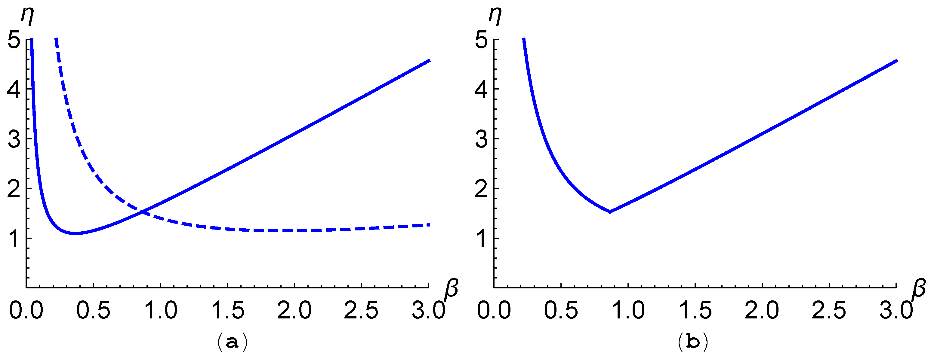
In the case $\mu =0$, the matrix $H_{\beta ,0}$ is diagonal, and therefore does not have a Perron–Frobenius eigenvalue. Instead the matrix $H_{\beta ,0}$ has the two eigenvalues

$$\beta D_d+{\beta }^{-1}{r}_d,\mathrm{and}\beta D_e+{\beta }^{-1}{r}_e,$$

(35)

which we plot in Figure 5a as functions of $\beta$ (for certain parameters). The minimum of the first curve in (35) is $2\sqrt{r_d{D}_d}$, which we note is the Fisher speed of the disperser $v_d$, and occurs at the $\beta$-value

$${\beta }_d=\sqrt{r_d/D_d}.$$

(36)

Similarly, the minimum of the second curve in (35) is the Fisher speed of the disperser $v_e=2\sqrt{r_e{D}_e}$, and occurs at the $\beta$-value

$${\beta }_e=\sqrt{r_e/D_e}.$$

(37)

The third point of interest is the point at which the the two curves in (35) cross, which is $v_f$, and occurs at the $\beta$-value

$${\beta }_f=\frac{\sqrt{r_e-r_d}}{\sqrt{D_d-D_e}}.$$

(38)

By analogy with the Perron–Frobenius eigenvalue we consider the maximum of these two eigenvalues for each $\beta$, which we plot in Figure 5b. Note here the similarity to the plot of the Perron–Frobenius eigenvalue of $H_{\beta ,\mu }$, seen in Figure 4.

Definition 2.

We define the minimum over β of the maximum function of eigenvalues defined in (35) to be ${\eta }_0$. Likewise, we denote the value of β at which this minimum is obtained by ${\beta }^{*}$.

Note that, in Figure 5, the minimum over $\beta$ of the maximum of the eigenvalues (35) is the point at which they both meet, and therefore in this case ${\eta }_0=v_f$ and ${\beta }^{*}={\beta }_f$.

However there are also regions of parameters in which the eigenvalues (35) meet in such a way that this is not the case. The condition that the minima of the two eigenvalues lie on either side of the point at which they meet, which is equivalent to the minimum value of $\beta$ of the maximum of the eigenvalues being at the crossing point, as in Figure 5, is

$$\sqrt{\frac{r_d}{D_d}}<\sqrt{\frac{r_e-r_d}{D_d-D_e}}<\sqrt{\frac{r_e}{D_e}},$$

(39)

which implies the condition

$$\frac{r_e}{r_d}+\frac{D_e}{D_d}>2\mathrm{and}\frac{r_d}{r_e}+\frac{D_d}{D_e}>2,$$

(40)

imposed by Elliott and Cornell [3] ensuring that the faster spreading speed $v_f$ (7) is obtained in the limit as $\mu \to 0$. Further, when condition (40) is satisfied, $H_{{\beta }^{*},0}$ is a multiple of the identity and has a repeated eigenvalue with a two-dimensional eigenspace. We consider this case, where $v_f$ is obtained as the limiting speed as $\mu \to 0$, to be of most biological interest, as unlike $v_e$ and $v_d$, $v_f$ is then dependent on the traits of both morphs and occurs as a result of polymorphism.

In the case that the condition (40) is not satisfied we would expect one of the individual speeds be selected. For example if the dispersal and growth rates of each phenotype satisfy

$$\frac{r_e}{r_d}+\frac{D_e}{D_d}<2\mathrm{and}\frac{r_d}{r_e}+\frac{D_d}{D_e}>2,$$

(41)

then the individual speed of phenotype d is selected. In this case the minimum over $\beta$ of the maximum of the eigenvalues (35) is no longer the crossing point of the eigenvalues, and is instead the minimum of the eigenvalue curve $\beta D_d+{\beta }^{-1}{r}_d$, therefore ${\eta }_0=v_d$ and ${\beta }^{*}={\beta }_d$. Similarly, in the case

$$\frac{r_e}{r_d}+\frac{D_e}{D_d}>2\mathrm{and}\frac{r_d}{r_e}+\frac{D_d}{D_e}<2,$$

(42)

where the individual speed of phenotype e is selected, we see that ${\eta }_0=v_e$ and ${\beta }^{*}={\beta }_e$. It is not possible for both inequalities in (40) to be reversed while the condition (2) holds.

Proposition 2.

If (40) holds, then ${\eta }_0=v_f$ and ${\beta }^{*}={\beta }_f$. If (41) holds, then ${\eta }_0=v_d$ and ${\beta }^{*}={\beta }_d$. If (42) holds, then ${\eta }_0=v_e$ and ${\beta }^{*}={\beta }_e$.

The values ${\eta }_0$ and ${\beta }^{*}$, defined in Definition 2 using the eigenvalues of the matrices $H_{\beta ,0}$, are shown in Morris [12] Theorems 5.6–5.11 to be the limits of $\eta \left(\mu \right)$ and $\beta \left(\mu \right)$ as the mutation rate $\mu \to 0$. In light of the linear determinancy of the spreading speed established in the works by the author of [11,12], this yields a rigorous characterisation of the limit of the spreading speed as $\mu \to 0$, which shows, in particular, that the limiting speeds (7) predicted by Elliott and Cornell [3] using the front propagation method of van Saarloos [21] are indeed what is obtained in the limit of small mutation. Here we summarise the results and refer to Theorems 5.6–5.11 of Morris [12] for details of the proofs.

Theorem 2.

In all three of the parameter regions (40)–(42),

$$\underset{\mu \to 0}{lim}\eta \left(\mu \right)={\eta }_0,\underset{\mu \to 0}{lim}\beta \left(\mu \right)={\beta }^{*},$$

where ${\eta }_0,{\beta }^{*}$ are as defined in Definition 2, that is,

(i) 

if (40) holds, then

$$\underset{\mu \to 0}{lim}\eta \left(\mu \right)=\frac{|r_e{D}_d-r_d{D}_e|}{\sqrt{(r_e-r_d)(D_d-D_e)}},\underset{\mu \to 0}{lim}\beta \left(\mu \right)=\frac{\sqrt{r_e-r_d}}{\sqrt{D_d-D_e}},$$

(ii) 

if (41) holds, then

$$\underset{\mu \to 0}{lim}\eta \left(\mu \right)=2\sqrt{r_d{D}_d},\underset{\mu \to 0}{lim}\beta \left(\mu \right)=\sqrt{r_d/D_d},$$

(iii) 

if (42) holds, then

$$\underset{\mu \to 0}{lim}\eta \left(\mu \right)=2\sqrt{r_e{D}_e},\underset{\mu \to 0}{lim}\beta \left(\mu \right)=\sqrt{r_e/D_e}.$$

Note that Tang and Fife [38] established the existence of travelling fronts for (1) for all speeds greater than or equal to $max\{2\sqrt{r_e{D}_e},2\sqrt{r_d{D}_d}\}$. Therefore, interestingly, in the case when (2) and (40) are satisfied, the limit as $\mu \to 0$ of the minimal front speed $\eta \left(\mu \right)$ is strictly larger than the minimal front speed for (1) in the absence of mutation.

Since calculating the spreading speed $\eta \left(\mu \right)$ involves minimizing in $\beta$ and the diffusion matrix A is not a multiple of the identity, finding an explicit expression for $\eta \left(\mu \right)$ is not very tractable. However, by adapting an argument from the work by the author of [37], we show that $\eta \left(\mu \right)$ is a nonincreasing function of the mutation rate $\mu$. A key ingredient of the proof is the following classical result of Cohen [39] on convexity properties of Perron–Frobenius eigenvalues.

Lemma 1

(Cohen [39]). Let $P,Q\in {\mathbb{R}}^{n\times n}$ such that P is diagonal and Q has positive off-diagonal elements. Then the Perron–Frobenius eigenvalue of $P+Q$ is a convex function of P; that is, given diagonal matrices $P_1$ and $P_2$ and $0<\alpha <1$,

$${\eta }_{\mathrm{PF}}(\alpha P_1+(1-\alpha )P_2+Q)\le \alpha {\eta }_{\mathrm{PF}}(P_1+Q)+(1-\alpha ){\eta }_{\mathrm{PF}}(P_2+Q).$$

(43)

This convexity, together with the fact that ${\eta }_{PF}\left(M\right)=0$, can now be exploited to obtain the following.

Theorem 3.

$\eta \left(\mu \right)$ is a nonincreasing function of μ.

Proof. 

Take ${\mu }_0>0$, define Z to be the $2\times 2$ zero matrix, and define

$$P:=\beta {\left({\mu }_0\right)}^{2}A-\beta \left({\mu }_0\right)\eta \left({\mu }_0\right)I+g^{\prime }\left(0\right)$$

(44)

Note that $\beta \left({\mu }_0\right)>0$ and

$$\begin{array}{cc}\hfill {\eta }_{\mathrm{PF}}({\beta }^{2}A-\beta \eta \left({\mu }_0\right)I+g^{\prime }\left(0\right)+{\mu }_{0}M)& \ge 0,\forall \beta >0,\hfill \end{array}$$

(45)

$$\begin{array}{cc}\hfill {\eta }_{\mathrm{PF}}(\beta {\left({\mu }_0\right)}^2-\beta \left({\mu }_0\right)\eta \left({\mu }_0\right)I+g^{\prime }\left(0\right)+{\mu }_{0}M)& =0.\hfill \end{array}$$

(46)

Now for any $\mu >0$, we know that

$${\eta }_{\mathrm{PF}}\left(P+\mu M\right)=\mu {\eta }_{\mathrm{PF}}\left(\frac{1}{\mu }P+M\right),$$

(47)

and in particular, ${\eta }_{\mathrm{PF}}(P+\mu M)$ and ${\eta }_{\mathrm{PF}}\left(\frac{1}{\mu }P+M\right)$ have the same sign. Moreover,

$${\eta }_{\mathrm{PF}}\left(\frac{1}{{\mu }_0}P+M\right)=0.$$

(48)

For any $\mu >{\mu }_0$, we can write,

$$\frac{1}{\mu }P=\frac{{\mu }_0}{\mu }\left(\frac{1}{{\mu }_0}P\right)+\left(1-\frac{{\mu }_0}{\mu }\right)Z.$$

(49)

Now in Lemma 1, let $P/{\mu }_0$ and Z be $P_1$ and $P_2$, respectively, and let $\alpha :={\mu }_0/\mu$. Then by the convex dependence of ${\eta }_{\mathrm{PF}}$,

$$\begin{array}{cc}\hfill {\eta }_{\mathrm{PF}}\left(\frac{1}{\mu }P+M\right)& \le \frac{{\mu }_0}{\mu }{\eta }_{\mathrm{PF}}\left(\frac{1}{{\mu }_0}P+M\right)+\left(1-\frac{{\mu }_0}{\mu }\right){\eta }_{\mathrm{PF}}\left(Z+M\right)\hfill \\ \hfill & =\frac{{\mu }_0}{\mu }{\eta }_{\mathrm{PF}}\left(\frac{1}{{\mu }_0}P+M\right)+\left(1-\frac{{\mu }_0}{\mu }\right){\eta }_{\mathrm{PF}}\left(M\right).\hfill \end{array}$$

(50)

We know from (48) that the first term is equal to zero, and ${\eta }_{\mathrm{PF}}\left(M\right)=0$ implies the second term is also zero. The inequality (50) therefore becomes

$${\eta }_{\mathrm{PF}}\left(\frac{1}{\mu }P+M\right)\le 0,\mu >{\mu }_0.$$

(51)

Using (47), this implies

$${\eta }_{\mathrm{PF}}\left(P+\mu M\right)\le 0,\mu >{\mu }_0,$$

(52)

and substituting in the full expression for P and dividing by $\beta \left({\mu }_0\right)$ then yields

$${\eta }_{\mathrm{PF}}(\beta \left({\mu }_0\right)A+\beta {\left({\mu }_0\right)}^{-1}(g^{\prime }\left(0\right)+\mu M))\le \eta \left({\mu }_0\right),\mu >{\mu }_0.$$

(53)

Hence

$$\underset{\beta >0}{inf}{\eta }_{\mathrm{PF}}(\beta A+{\beta }^{-1}(g^{\prime }\left(0\right)+\mu M))\le \eta \left({\mu }_0\right).$$

(54)

Since the expression on the left hand side of (54) is the definition of $\eta \left(\mu \right)$, we have

$$\eta \left(\mu \right)\le \eta \left({\mu }_0\right).$$

(55)

Since this holds for any $\mu >{\mu }_0$, we have therefore shown that $\eta \left(\mu \right)$ is a nonincreasing function of $\mu$. □

In light of the linear determinancy of the spreading speed [11,12], Theorem 3 establishes that the spreading speed for the nonlinear system (1) is a nonincreasing function of the mutation rate $\mu$. Interestingly, this is related mathematically to the so-called “reduction phenomenon” discussed by Altenberg [29], which roughly says that, under certain conditions, greater mixing results in lowered growth. On the other hand, our result can be interpreted as showing that greater mixing results in a slower speed of propagation. It is possible, in fact, to make use of Theorem 6(iii) [29] to give a slightly different proof of Proposition 3.

4. Behaviour at the Leading Edge in the Limit μ → 0

Here we study the Perron–Frobenius eigenvector $q_{\beta }\left(\mu \right)$ corresponding to the eigenvalue $\eta \left(\mu \right)$ in the limit as the mutation rate $\mu \to 0$, with the aim of determining the ratio of the phenotypes in the leading edge of an invasion. We do this under conditions (2) and (8) on the dispersal and growth parameters, which, by Theorem (2)(i), ensures that the faster speed $v_f$ is obtained as $\mu \to 0$ and, as we will see, results in both phenotypes being present in the leading edge. Throughout this section we therefore assume that

$$\frac{r_e}{r_d}+\frac{D_e}{D_d}>2\mathrm{and}\frac{r_d}{r_e}+\frac{D_d}{D_e}>2,$$

(56)

as well as

$$r_e>r_d,D_d>D_e,$$

(57)

and for convenience in the following, define the quantities

$$a:={\beta }^{{*}^2}{D}_d-r_d,b:=-{\beta }^{{*}^2}{D}_e+r_e.$$

(58)

Note that a straightforward calculation shows that the condition

$$a>0\mathrm{and}b>0$$

(59)

is equivalent to the condition (56). We consider this parameter regime to be of greatest biological interest, since unlike $v_e$ and $v_d$, the value $v_f$ is dependent on the traits of both morphs and occurs as a result of polymorphism. Note that it is shown by (Girardin [40], Theorem 1.1) that the eigenvector $q_{\beta }\left(\mu \right)$, which arises in the explicit solution of the linearised problem (29), does indeed also characterise the asymptotic behaviour of travelling wave solutions of the nonlinear system (1) close to the extinction state.

In the absence of mutation ($\mu =0$), Figure 5 illustrates the $\beta$-dependence of eigenvalues of the matrix $H_{\beta ,0}$ for a choice of dispersal and growth parameters for which conditions (56) and (57) are satisfied. Under these conditions, the minimal travelling wave speed ${\eta }_0$ is obtained at the point at which the two eigenvalues of $H_{\beta ,0}$ meet, so that

$${\eta }_0={\beta }^{*}{D}_d+{\beta }^{{*}^{-1}}{r}_d={\beta }^{*}{D}_e+{\beta }^{{*}^{-1}}{r}_e,{\beta }^{*}=\sqrt{\frac{r_e-r_d}{D_d-D_e}}.$$

(60)

In this case, $H_{{\beta }^{*},0}$ is a multiple of the identity, so has a repeated eigenvalue with a two-dimensional eigenspace, making it not obvious a priori what ratio between the two components one would expect in the limit of vanishing mutation.

We therefore investigate the Perron–Frobenius eigenvector q of $H_{\beta \left(\mu \right),\mu }$ in the limit $\mu \to 0$, restricting attention to the region of parameters in which (56) and (57) hold. Recall from Theorem 2 that ${lim}_{\mu \to 0}\eta \left(\mu \right)={\eta }_0$ and ${lim}_{\mu \to 0}\beta \left(\mu \right)={\beta }^{*}$, and assume that the following limits exist.

$${\eta }^{\prime }\left(0\right)=\underset{\mu \to 0}{lim}\frac{\eta \left(\mu \right)-{\eta }_0}{\mu },{\beta }^{\prime }\left(0\right)=\underset{\mu \to 0}{lim}\frac{\beta \left(\mu \right)-{\beta }^{*}}{\mu }.$$

(61)

Note that we provide further numerical justification of these assumptions in Figure 6. Rewriting (30) as a system of scalar equations and taking $\beta =\beta \left(\mu \right)$, we obtain

$$\begin{array}{cc}\hfill \left(\beta \left(\mu \right)D_e+\frac{(r_e-\mu e)}{\beta \left(\mu \right)}-\eta \left(\mu \right)\right)+\frac{\mu d}{\beta \left(\mu \right)}\frac{q_2}{q_1}& =0,\hfill \end{array}$$

(62)

$$\begin{array}{cc}\hfill \left(\beta \left(\mu \right)D_d+\frac{(r_d-\mu d)}{\beta \left(\mu \right)}-\eta \left(\mu \right)\right)\frac{q_2}{q_1}+\frac{\mu e}{\beta \left(\mu \right)}& =0,\hfill \end{array}$$

(63)

for $\mu >0$. Then adding and subtracting ${\eta }_0$ from (62) and (63), and dividing by $\mu \beta {\left(\mu \right)}^{-1}$ yields

$$\begin{array}{c}\hfill {\beta }^{*}\frac{(\beta D_e+{\beta }^{-1}{r}_e)-({\beta }^{*}{D}_e+{\beta }^{{*}^{-1}}{r}_e)}{\mu }-{\beta }^{*}\frac{\eta -{\eta }_0}{\mu }-e+d\frac{q_2}{q_1}=0\end{array}$$

(64)

$$\begin{array}{c}\hfill \left({\beta }^{*}\frac{(\beta D_d+{\beta }^{-1}{r}_d)-({\beta }^{*}{D}_d+{\beta }^{{*}^{-1}}{r}_d)}{\mu }-{\beta }^{*}\frac{\eta -{\eta }_0}{\mu }-d\right)\frac{q_2}{q_1}+e=0\end{array}$$

(65)

Now bearing in mind (61) and the fact that ${\beta }^{*}\ne 0$, it follows from (64) that

$$\frac{q_{0_2}}{q_{0_1}}:=\underset{\mu \to 0}{lim}\frac{q_2}{q_1}$$

exists, so that taking the limit $\mu \to 0$ in (64), (65), we obtain a system of two equations in the three unknowns $q_{0_2}/q_{0_1}$, ${\eta }^{\prime }\left(0\right)$ and ${\beta }^{\prime }\left(0\right)$,

$$\begin{array}{cc}\hfill {\beta }^{*}\left[D_e{\beta }^{\prime }\left(0\right)-\frac{r_e{\beta }^{\prime }\left(0\right)}{{\beta }^{{*}^2}}-{\eta }^{\prime }\left(0\right)\right]-e+d\left(\frac{q_{0_2}}{q_{0_1}}\right)& =0,\hfill \end{array}$$

(66)

$$\begin{array}{cc}\hfill {\beta }^{*}\left[D_d{\beta }^{\prime }\left(0\right)-\frac{r_d{\beta }^{\prime }\left(0\right)}{{\beta }^{{*}^2}}-{\eta }^{\prime }\left(0\right)\right]\left(\frac{q_{0_2}}{q_{0_1}}\right)-d\left(\frac{q_{0_2}}{q_{0_1}}\right)+d& =0.\hfill \end{array}$$

(67)

To obtain a third equation, recall that the eigenvalues $\lambda$ of $H_{\beta ,\mu }$ satisfy $det(H_{\beta ,\mu }-\lambda I)=0$, so that

$$(\lambda -\beta D_e-{\beta }^{-1}(r_e-\mu e))(\lambda -\beta D_d-{\beta }^{-1}(r_d-\mu d))-{\beta }^{-2}{\mu }^{2}ed=0,$$

(68)

and further, at $\beta =\beta \left(\mu \right)$, we have

$$\frac{\partial \lambda }{\partial \beta }=0,\mathrm{when}\lambda =\eta \left(\mu \right).$$

(69)

Differentiating (68) with respect to $\beta$ and setting $\beta =\beta \left(\mu \right)$, $\lambda =\eta \left(\mu \right)$, we then multiply the result by ${\beta }^3$ to obtain

$$\begin{array}{c}({\beta }^2(D_e+D_d)-(r_e+r_d-\mu e-\mu d))\beta \eta \left(\mu \right)-2{\mu }^{2}ed=\hfill \\ ({\beta }^2{D}_e-(r_e-\mu e))({\beta }^2{D}_d+(r_d-\mu d))+({\beta }^2{D}_e+(r_e-\mu e)({\beta }^2{D}_d-(r_d-\mu d)).\hfill \end{array}$$

(70)

Then differentiating with respect to $\mu$ and letting $\mu \to 0$ yields a third equation relating ${\beta }^{\prime }\left(0\right)$ and ${\eta }^{\prime }\left(0\right)$, namely

$$2{\beta }^{*}(b{D}_d-a{D}_e){\beta }^{\prime }\left(0\right)+{\eta }_0(a-b){\beta }^{\prime }\left(0\right)+{\beta }^{*}(a-b){\eta }^{\prime }\left(0\right)=(bd-ae),$$

(71)

where a and b are as defined in (58). Recall from (59) that $a,b$ are both positive due to the assumption (56) on the parameters $D_e,D_d,r_e$ and $r_d$.

We thus have a system of three equation (66), (67) and (71), which we solve. Eliminating ${\eta }^{\prime }\left(0\right)$ and ${\beta }^{\prime }\left(0\right)$ gives the explicit expression for $q_{0_2}/q_{0_1}$:

$$q_{\mathrm{ratio}}:=\frac{q_{0_2}}{q_{0_1}}=\sqrt{\frac{be}{ad}}=\sqrt{\frac{(r_e-{\beta }^{*2}{D}_e)e}{({\beta }^{*2}{D}_d-r_d)d}}>0.$$

(72)

Recall that this is the ratio of the two components of the eigenvector of (30) in the limit $\mu \to 0$, where $q_2$ represents the disperser and $q_1$ the establisher. This quantity therefore predicts the ratio of the two morphs present in the leading edge of the minimal-speed travelling wave solution to our system [40], which gives insight into the expected long-time behaviour of the solution of (1) with Heaviside initial conditions that models the invasion of the two morphs into an empty region. Note that since $q_{\mathrm{ratio}}>0$, both morphs play a role in the leading edge.

The presence of the two positive quantities a and b in (72) emphasizes that this expression holds only in the zone where (56), which is equivalent to (59), is satisfied, in which case the faster speed $v_f$ is obtained in the limit $\mu \to 0$. If instead either condition (41) or condition (42) holds, in which case the $\mu \to 0$ limits of $\beta \left(\mu \right)$ and $\eta \left(\mu \right)$ are given by Theorem 3.5 (ii) or (iii) and depend either only on $D_e,r_e$ or only on $D_d,r_d$, then up to normalisation, the $\mu \to 0$ limit $q_0$ of the eigenvector $q_{\beta }\left(\mu \right)$ is either ${(1,0)}^T$ or ${(0,1)}^T$, corresponding to $q_{\mathrm{ratio}}=0$ or ∞. This is because the diagonal matrix $H_{{\beta }^{*},0}=diag({\beta }^{*}{D}_e+\frac{r_e}{{\beta }^{*}},{\beta }^{*}{D}_d+\frac{r_d}{{\beta }^{*}})$ is then no longer a multiple of the identity and the eigenvector $q_0$ satisfies $H_{{\beta }^{*},0}{q}_0={\eta }_0{q}_0$. So in these parameter zones, one of the two phenotypes will dominate the leading edge of the front in the limit $\mu \to 0$, in contrast to the zone when (56) holds, when (72) is valid and both components play a role.

4.1. Discussion of Leading Edge Behaviour

In order to investigate the effects of parameters on the proportion of each morph in the leading edge, note that using the substitutions $r=r_d/r_e$, $D=D_e/D_d$, $m=e/d$, we can rewrite (72) as a function of only three variables, the ratio of the growth rates r, the ratio of the dispersal rates D, and the ratio of the mutation rates m, namely,

$$q_{\mathrm{ratio}}=\sqrt{\left(\frac{2D-rD-1}{2r-rD-1}\right)m}.$$

(73)

This is both biologically interesting and mathematically elegant.

It is instructive and biologically relevant to comment on the effect on $q_{\mathrm{ratio}}$ of varying parameters r, D, and m. Figure 7 illustrates how the ratio of growth, dispersal and mutation rates affects the proportion of each morph in the leading edge of the invasion wave.

We see in Figure 7a that as $r_e$ increases (or $r_d$ decreases) there is an increase in the establisher morph in the leading edge. However, as $q_{\mathrm{ratio}}$ does not fall below 1, there is always a larger amount of the disperser morph in the leading edge. As we increase $r_e$ to infinity (or decrease $r_d$ to 0) $q_{\mathrm{ratio}}$ tends to $\sqrt{(1-2/D)m}$. Observe also that in (i), $q_{\mathrm{ratio}}$ blows up at the value of $r=r_d/r_e$ at which, for the fixed value of $D=D_e/D_d$ in the plot, our assumption that $a>0$ and $b>0$ stops holding. This corresponds to the (normalised) eigenvector $q_0$ approaching the eigenvector ${(0,1)}^T$ and the parameters $D,r$ entering the zone where (41) holds and ${lim}_{\mu \to 0}\eta \left(\mu \right)$ is the Fisher speed of the disperser morph $v_d$ instead of $v_f$.

Figure 7b tells us that as we increase $D_d$ (or decrease $D_e$), there is an increase in the disperser morph in the leading edge. If $D_e$ and $D_d$ are close enough in value, it is possible that the establisher morph outnumbers the disperser in the leading edge, which we see in the region in which $q_{\mathrm{ratio}}$ drops below one. As we increase $D_d$ to infinity (or decrease $D_e$ to 0) $q_{\mathrm{ratio}}$ tends to $\sqrt{m/(1-2r)}$. In the case of (ii), the ratio $q_{\mathrm{ratio}}$ becomes zero at the value of $D=D_e/D_d$ at which, for the fixed value of $r=r_d/r_e$ in the plot, our assumption that $a>0$ and $b>0$ no longer holds. This corresponds to the (normalised) eigenvector $q_0$ approaching the eigenvector ${(1,0)}^T$ and the parameters $D,r$ entering the zone where (42) holds and ${lim}_{\mu \to 0}\eta \left(\mu \right)$ is the Fisher speed of the establisher morph $v_e$ instead of $v_f$.

In Figure 7c we see that if the mutation rate of a morph is increased it results in a decrease in the density of that morph in the leading edge. Since the ratio m is not restricted to a particular range, like r and D due to (2), we see that the mutation rate is also able to change which morph is more prevalent in the leading edge. If we fix all parameters but the mutation rates in (73) we obtain $q_{\mathrm{ratio}}=\sqrt{km}$, where $k>0$ is a constant. Thus $q_{\mathrm{ratio}}$ goes to zero as m grows smaller and blows up as m tends to infinity. These provide us with interesting predictions which could be tested experimentally with real biological systems.

Note that, of course, the results of the works by the authors of [11,12] on linear determinacy and existence of travelling waves are valid for all parameter choices $D_e,D_d,r_e,r_d$. The fact that the expression $q_{\mathrm{ratio}}$ only holds in some parameter zones is just an expression of the fact that only for certain parameters does the eigenvector that describes the leading edge of the front, which is strictly positive whenever $\mu >0$, tend to a strictly positive eigenvector as $\mu \to 0$.

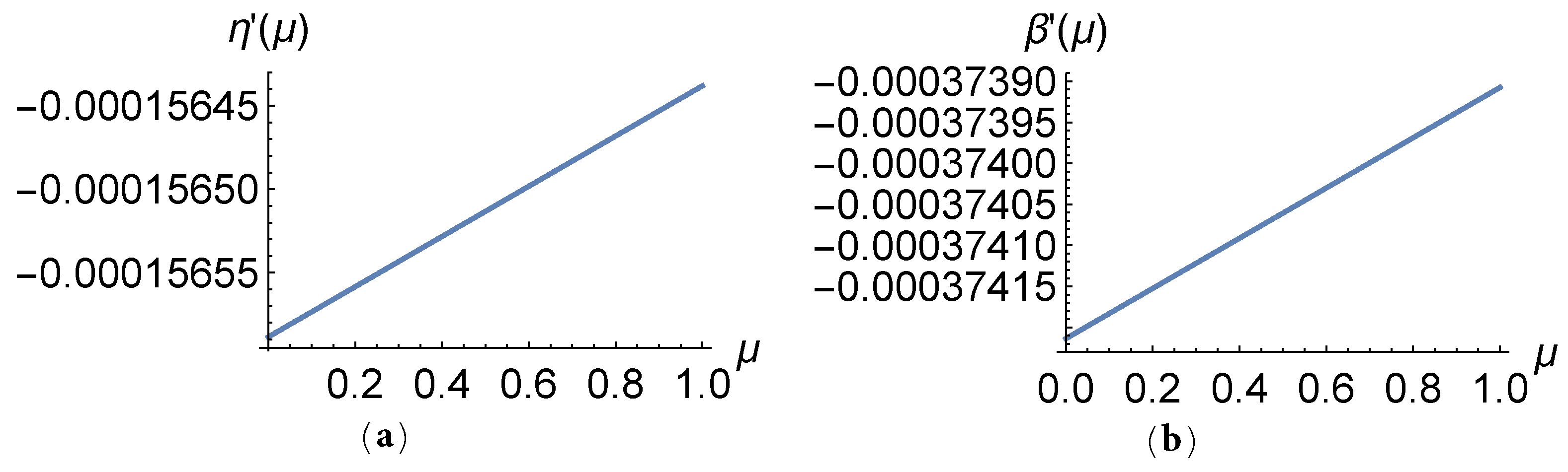
Recall that we made assumptions (61) on the existence of ${\eta }^{\prime }\left(0\right)$ and ${\beta }^{\prime }\left(0\right)$, for which we now provide some justification by numerically solving Equations (62), (68) and (70) as a system of three equations in $q_2/q_1$, $\eta \left(\mu \right)$ and $\beta \left(\mu \right)$. Differentiating the latter two with respect to $\mu$ we plot ${\eta }^{\prime }\left(\mu \right)$, ${\beta }^{\prime }\left(\mu \right)$ and $q_2/q_1$ as functions of $\mu$ in Figure 6 demonstrating the existence of ${\eta }^{\prime }\left(0\right)$, ${\beta }^{\prime }\left(0\right)$ and $q_{\mathrm{ratio}}$ for this set of parameters. Note that as $\mu$ increases we see an increase in the proportion of the phenotype $n_d$, which is expected as for this set of parameters $e>d$.

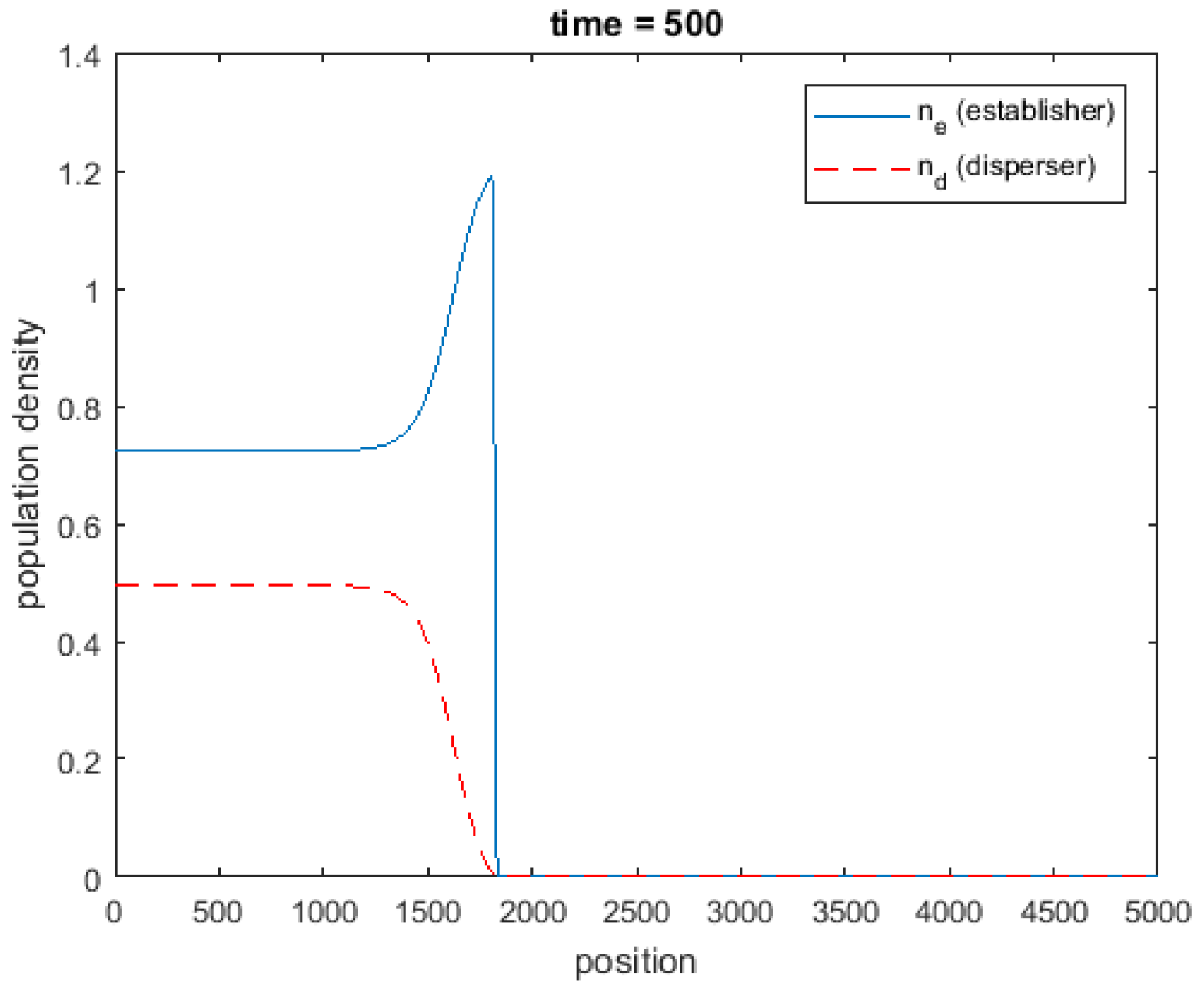
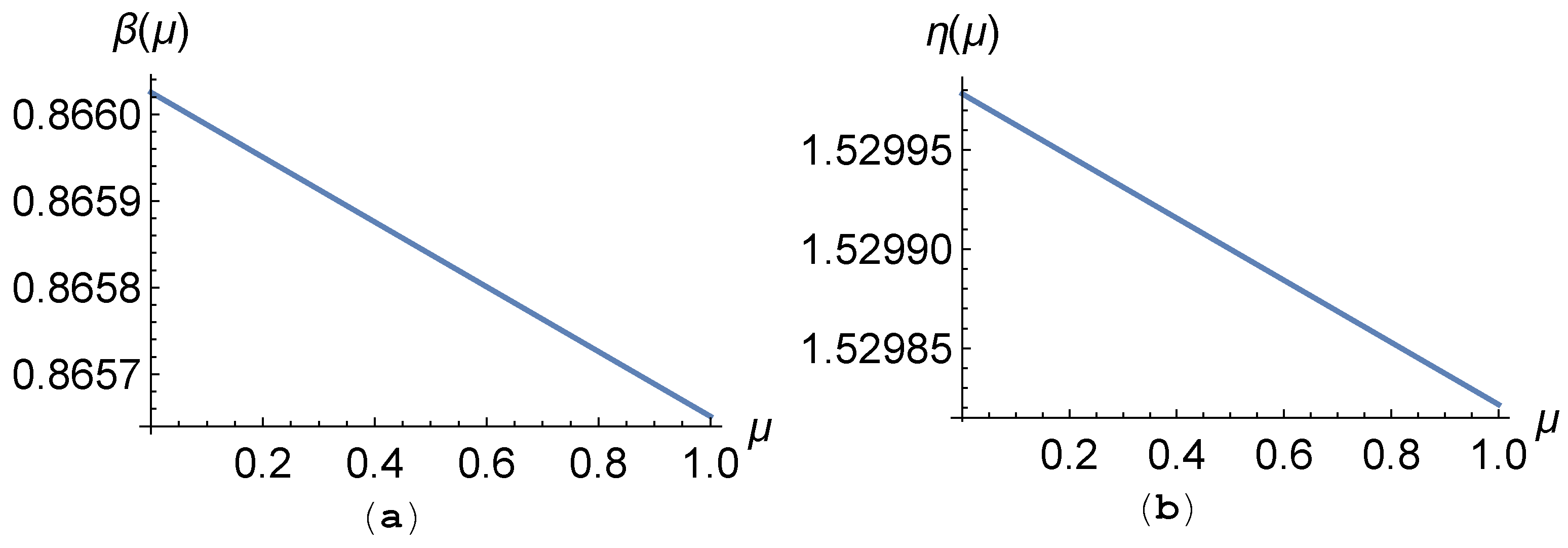
Finally, we also plot $\beta \left(\mu \right)$ and $\eta \left(\mu \right)$ as functions of $\mu$ in Figure 8. As $\mu \to 0$ we see $\beta \left(\mu \right)$ and $\eta \left(\mu \right)$ converge to the values ${\beta }^{*}$ and ${\eta }_0$, respectively. Further, as we increase $\mu$ we observe a decrease in the minimal spreading speed $\eta \left(\mu \right)$, this is consistent with our result in Section 4.1.

5. Conclusions and Remarks

This article exploits linear determinacy of the competition–diffusion-mutation system (1) to establish ecologically-motivated results about the invasion properties of a species with two morphs. These results constitute theoretical predictions of the model, of which the most significant are

(i)

the spreading speed decreases as the mutation rate increases;

(ii)

there are three possible spreading speeds in the limit of vanishing mutation rate, the choice of which depends on the dispersal and growth parameters; and

(iii)

the ratio of the phenotypes in the leading edge of the invasion.

It would, of course, be valuable to compare these predictions with experimental or empirical data. Note that on the one hand, for the parameter regime (40), so-called ‘anomalous spreading’ in [3], the spreading speed in the vanishing mutation limit is faster than either phenotype would spread in isolation. On the other hand, once mutation is present, the spreading speed is a nonincreasing function of mutation. Although these predictions are rigorous consequences of the model, their juxtaposition is slightly counter-intuitive from an ecological point of view.

Activity on propagation phenomena in models incorporating mutation has increased markedly in recent years (see the works by the authors of [10,11,30,40] and many others) and is producing a growing body of interesting results and open questions. A natural progression of our work would be a detailed analysis of systems for N morphs, in particular, dependence of spreading speeds and the composition of the morphs in the leading edge on parameters. The methods developed in Section 3 and Section 4 have the clear potential to yield results in the N morph case. Also interesting is the role of functional trade-offs in determining spreading speeds in competition–diffusion mutation models, some first results on which are established in [12]. More wide-ranging questions include how best to model mutation (for instance, should the rate $\mu$ be replaced by a density-dependent rate), whether continuous or discrete trait models are most appropriate in a given setting, and how to pass rigorously from a discrete setting with a large number of traits to the continuous-trait setting.