1. Introduction
In industry, components are becoming more reliable due to rapid advances in manufacturing technology and sustained quality-improvement efforts. Practitioners have been encouraged to adopt censoring schemes for lifetime testing to save time and cost for making reliability inferences. Numerate censoring schemes, such as the first failure, group, type II, and progressive type II censoring schemes have been developed in the past years. Readers can refer Balakrishnan and Aggarwala [
1] as well as Balasooriya [
2] for more information. Considering the advantages from the first failure and progressive type II censoring schemes, a censoring scheme called progressive first failure-censoring scheme was studied by Lio and Tsai [
3] for the Burr type XII distribution and by Wu and Kuş [
4] for the Weibull distribution. Wu and Kuş [
4] demonstrated that the progressive first failure-censoring scheme is more efficient than the progressive type II censoring scheme in terms of the total expected run time.
A progressive first failure-censoring scheme is implemented by placing n test units independently into m independent groups of size k, where , to be tested at the same initial time, labeled by , and by collecting r lifetimes through the following procedure: At the first failure time, from n items is observed; the group with that failed item along with a randomly selected groups are removed. At the next first failure time, from the rest groups is observed; the group with that failed item along with randomly selected groups are removed. This process continues until the rth first failure time is observed; then all remaining surviving items are removed from the life test. The lifetimes, , are progressively type II first failure-censored ordered statistics. Let , where .
Let the lifetimes of all test units follow a cumulative distribution function (cdf)
, which has the probability density function (pdf)
. The likelihood function based on a progressively first failure-censored sample can be presented by
where
The likelihood function in Equation (
1) covers the following as special cases:
If
, then Equation (
1) reduces to the the likelihood function of first failure-censored ordered statistics.
If
, then Equation (
1) becomes the likelihood function of progressively type II-censored statistics.
If
and
, then
and Equation (
1) is the likelihood function of complete sample.
If
and
, then Equation (
1) simplifies to the likelihood function of type II-censored order statistics.
In mechanical reliability, let
X be the “stress” that is applied to a certain component and
Y be the “strength” to sustain the stress. The stress–strength parameter can be denoted by
.
is comprised of components that receive a certain level of stress and that survive due to their strength. If a higher level of stress than their strength is able to sustain is applied, the component is broken-down. When the pdfs of the stress and strength variables are known, the reliability of the system may be determined analytically. Since a connection between the classical Mann–Whitney statistic and the stress–strength inference was mentioned by Birnbaum [
5], the estimation of
has received considerable attention in the statistical literatures. The statistical inferences of
for complete samples have been studied by Tong [
6], Surles and Padgett [
7], Kundu and Gupta [
8,
9], Raqab et al. [
10], Kim and Chung [
11], and Kundu and Raqab [
12]. The monograph by Kotz et al. [
13] provided an excellent review of the development of the stress–strength up to the year of 2003. Moreover, Saracoglu, and Kaya [
14] obtained the maximum likelihood equations and made interval inferences for
from two Gompertz distributions. Saracoglu et al. [
15] studied the comparison of the estimators of
for Gompertz cases.
Under incomplete samples, Jiang and Wong [
16] studied the inferences of
based on truncated exponentially distributed samples. Statistical inference for
based on progressively censored samples was discussed by Saracoglu and Ku̧s [
17]. Saracoglu et al. [
18] studied the estimation of
based on progressively type II censored samples from two independent exponential distributions. Lio and Tsai [
3] studied the inference of
for Burr type XII distributions based on progressively type II first failure-censored samples. All aforementioned studies focused on using maximum likelihood estimation methods.
The Burr type XII distribution is a popular lifetime model in reliability applications. For example, the Burr type XII distribution can be the lifetime model to infer the breaking strength of structure components. Burr [
19] first introduced the two-parameter Burr type XII distribution in the literature in 1942. The Burr type XII distribution includes another popular lifetime distribution in reliability analyses, the loglogistic distribution, as a special case. The Burr type XII distribution contains two shape parameters. Hence, the Burr type XII distribution has flexible distribution shapes for model fitting. Based on our best knowledge, this is the first work that focuses on using Bayesian methods for inferring
. The rest of this paper is organized as follows. The Burr type XII distribution and Bayesian framework are described in
Section 2. In
Section 3, the Metropolis–Hastings (M–H) algorithm (Metropolis et al. [
20] and Hastings [
21]) via Gibbs sampling (Geman and Geman [
22]) is developed by using the joint distribution of progressively first failure-censored sample and the joint prior distribution of Burr type XII parameters to collect the random sample of
that is generated from the posterior distribution of
, and the Bayes estimates under the square error (SE), absolute error (AE), and linear exponential error (Linex) loss functions are developed using the empirical distribution of the collected random sample of
. In
Section 4, an intensive simulation procedure is conducted under different censoring schemes to compare the performances among the three Bayes point estimators mentioned in
Section 2 as well as to investigate the credible intervals of
. Moreover, simulations are also conducted to compare the performances of the proposed Bayesian estimation method with the maximum likelihood estimation in
Section 4. The Internet of Things (IoT) applications and the reliability evaluation about the miles-to-failure of vehicle components are presented in
Section 5 for illustration. Finally, some concluding remarks are provided in
Section 6.
2. Statistical Approaches
Let
X and
Y follow independent Burr type XII distributions, which have the following pdfs,
and
respectively, and the cdfs of
X and
Y are respectively denoted as
and
The stress–strength parameter can be obtained by
When
,
can be shown to be
2.1. Likelihood Function
Let the progressively type II first-censored sample for
X and
Y be
, and let
R and
R denote the
and
removals for
X and
Y, respectively, where
and
. Then, the likelihood function for the data when
is
where
,
,
, and
.
2.2. Bayesian Framework
Because of the conditions of
,
and
, the prior distributions of
,
, and
are reasonably assumed as the following Gamma distributions:
where
and
are positive hyper-parameters. The Gamma distributions have been suggested to be the prior distributions of Burr type XII distribution parameters in the literature, for example, Panahi and Sayyareh [
23]. In practice, we can select the values of
and
for
such that the prior distribution has large variance and turns to be a non-informative prior. Given Equations (
9)–(
12), the joint posterior distribution can be represented as
Hence, the marginal posterior of
,
, and
are, respectively,
and
The conditional posterior of
given
and
is
the conditional posterior of
given
and
is
and the conditional posterior of
given
and
is
Unfortunately, the conditional posterior distributions
,
, and
do not have closed forms. Additionally, numerical integration cannot be easily applied to obtain the analytical expressions of these three conditional posterior distributions due to the commonly shared parameter
in two Burr type XII distributions.
Section 3 will address the Markov Chain Monte Carlo (MCMC) method that uses the M–H algorithm via Gibbs sampling to draw the samples of
,
,
, and
. Moreover, we also provide a function “
” by using OpenBugs R codes to overcome the difficulties caused by the commonly shared parameter
in numerical computation. On the basis of the MCMC random samples, the Bayes estimates of
,
,
, and
can be obtained with the SE, AE, and Linex loss functions through using the established formulas in
Section 3.
3. Markov Chain Monte Carlo
The MCMC procedure escapes the integration problem from the complicated marginal posterior distributions in Bayesian estimation by combining Markov chains and Monte Carlo sampling. In general, Markov chains are formed by taking a collection of random variables or states with the property that, given the present, the future is conditionally independent of the past. Probabilities from each state in a Markov chain are then called transition probabilities. In this study, there is a Markov chain for different states for each parameter in
, where
. Monte Carlo methods are a broad class of computational algorithms that rely on repeated random sampling to obtain numerical results. One such algorithm is M–H. In the M–H algorithm, the samples will mostly move towards higher density regions, which will hopefully contain the true analytic value for each parameter. Gibbs sampling is a particular case of the M–H algorithm that is common with Bayesian estimation. It generates samples from the marginal posteriors for each parameter by iteratively sampling from its conditional distribution with the remaining variables fixed to their current values until the convergence is achieved. We mentioned in
Section 2 that the conditional posterior distributions do not have closed forms and that the difficulties in numerical computation are caused by the commonly shared parameter
. In order to generate observations from the marginal posterior distributions, we adapt the arguments proposed by Lin et al. [
24] to develop the MCMC procedure. In this study, the M–H algorithm in the proposed MCMC procedure is implemented via using Gibbs samplings by the following steps:
Let and be the initial state , .
- Step 1:
Propose transition probabilities from to , where is usually selected as a symmetry function of at for
- Step 2:
Implement Step 3 and Step 4 for , where N is a huge number.
- Step 3:
For iteration
, Generate
from
and generate
u from the uniform distribution over the interval
. Update
according to the condition
where
,
,
, and
- Step 4:
Let .
It is noticed that the convergence can be reached when 40,000 for the implementation of the proposed MCMC algorithm. To ensure convergence is achieved, the OpenBugs program in R can be applied to implement the MCMC procedure stated above and to decide optimally through the utilization of the following procedure called mtemp, which contains likelihood function and priors for .
mtemp<-function(){
for (j in 1:r1)
{
for(i in 1:r2){
dummyy[j,i] <- 0
dummyy[j,i] ~ dloglik(logLikexy[j,i])
logLikexy[j,i] <- (log($\beta_1$)+log($\alpha$)+($\alpha$ -1.0)*log(x[j])
-($\beta_1$*k1*(R.x[j]+1.0)+1.0)*log(1.0 + pow(x[j],$\alpha$)))/r2
+(log($\beta_2$)+log($\alpha$)+($\alpha$ - 1.0)*log(y[i])
-($\beta_2$*k2*(R.y[i]+1.0)+1.0)*log(1.0 + pow(y[i],$\alpha$)))/r1
}}
$\beta_1$ ~ dgamma(0.000008, 0.0001)
$\beta_2$ ~ dgamma(0.000008, 0.0001)
$\alpha$ ~ dgamma(0.0005, 0.0001)
}
Please note that the function
mtemp using a zeros trick (see Lunn et al. [
25]) to define a custom distribution for the likelihood function due to the Burr type XII distribution was not a built-in distribution in OpenBugs.
Bayesian Estimates
In order to obtain reliable samples of the parameters,
,
and
from posteriors,
N Markov chains for each parameter are generated through the proposed MCMC procedure for each given pair of progressively first failure-censored samples,
and the first
are removed for burn-in. Let the resulting Markov chains of
after a burn-in process be
for
. Then, the corresponding chain of
can be expressed by
, where
for
. According to Lin et al. [
24],
for
and
can be used to construct the respective empirical distributions to estimate the corresponding posteriors. Therefore, the Bayes point estimates of
for
and
can be obtained based on the SE, AE, and Linex loss functions as follows:
Bayes Estimates under the SE Loss Function: Let the loss functions of
be
and the loss function for
be
. Then, the Bayes estimators of
under the SE loss function can be obtained as the posterior mean and calculated by
Similarly, the Bayes estimator of
can be obtained by
Bayes Estimates under the AE Loss Function: Let the loss functions of
be
and the loss function of
be
. Then, the Bayes estimators of
under the AE loss function is the posterior medians and can be calculated by
Similarly, the Bayes estimator of
can be obtained by
Bayes Estimates under the Linex Loss Function: Let the loss functions of
be
for
and the loss function of
be
, where
. The Bayes estimators of
under the Linex loss function can be obtained by
Similarly, the Bayes estimator of
can be obtained by
For , the Linex loss function is quite asymmetric about 0 with overestimation being more costly than underestimation. The vice versa is true with . When a is close to zero, the estimation results under the Linex loss function are close to that obtained under the SE loss function. In this study, we select to implement the MCMC algorithm.
For interval estimate, given , an credible interval of a parameter in the Bayesian framework is an interval estimator, based on a given data, that covers the parameter with levels of confidence. Symmetric credible intervals for and can be estimated by the credible intervals obtained through taking two symmetric tail cuts from each respective empirical distribution as the lower and upper bounds.
4. Simulation Study Results
Monte Carlo simulations are conducted based on the different progressive first failure-censoring schemes proposed by Wu and Kus [
4] and used by Lio and Tsai [
3]. The first simulation scenario uses a pair of Burr Type XII distributions with the parameters
and
, and the second simulation scenario uses a pair of Burr type XII distributions with the parameters
and
. The other simulation parameter inputs that are varied in each simulation scenario include the number of groups,
; the size of each group,
; and the number of observed lifetimes,
. The same progressive censoring schemes,
, are considered for the simulation study. Therefore, the simulation study has 36 combination settings that are labeled from 1 to 36 and displayed in
Table 1,
Table 2,
Table 3,
Table 4 and
Table 5.
The Bayes estimates for the parameters , , and and can be obtained based on the respective empirical distributions of the samples that are generated by the proposed MCMC procedure with the SE, AE, and Linex loss functions. The size of the Markov chain for implementing the MCMC procedure is N = 50,000 with = 40,000 chains for burn-in. The last Markov chains are used to establish the empirical distribution to estimate the posterior distribution of the parameter. Then, the Bayes estimate under a specific loss function can be obtained based on the empirical posterior distribution of and the credible interval of can be estimated by using the two symmetric cuts from the same empirical posterior distribution of . The Bayes estimates of using the SE, AE, and Linex loss functions are denoted by , , and , respectively. Repeat the MCMC procedures 500 times to generate 500 respective Bayes estimates of , which are labeled by , , and , and 500 credit interval estimates of .
Because of the difference between the expected value of estimator and the parameter (bias), the expected SE (ESE) and expected AE (EAE) are the most common measurements to evaluate the accuracy of an estimator to the true parameter. Therefore, in order to evaluate and compare the performance among the aforementioned three Bayes estimators based on the progressively first failure-censored sample, the bias, the ESE, and EAE are used to evaluate the accuracies of these three Bayes estimators of . Let be an Bayes estimator of . The bias measures how far the Bayes estimator over- or underestimates the true , and ESE and EAE measure how well the Bayes estimator, , fit its true values under the SE and AE criterions, respectively. Additionally the coverage probability of the credible interval estimator for can be estimated from the relative frequency of all 500 credible intervals that cover the true based on the empirical distributions. The average length from all simulated 500 credible intervals and the average lengths from all simulated credible intervals that cover the true parameter are also obtained for comparison.
Section 4.2 discusses the evaluation of the bias of
,
Section 4.2,
Section 4.3 and
Section 4.4 investigate the ESE and EAE for the three Bayes estimators of
.
Section 4.5 discusses the procedure related to the credible intervals of
along with their coverage probabilities and average lengths. The estimation performance of the Bayesian estimation method via use of the proposed MCMC procedure is compared with the maximum likelihood estimation method in
Section 4.6.
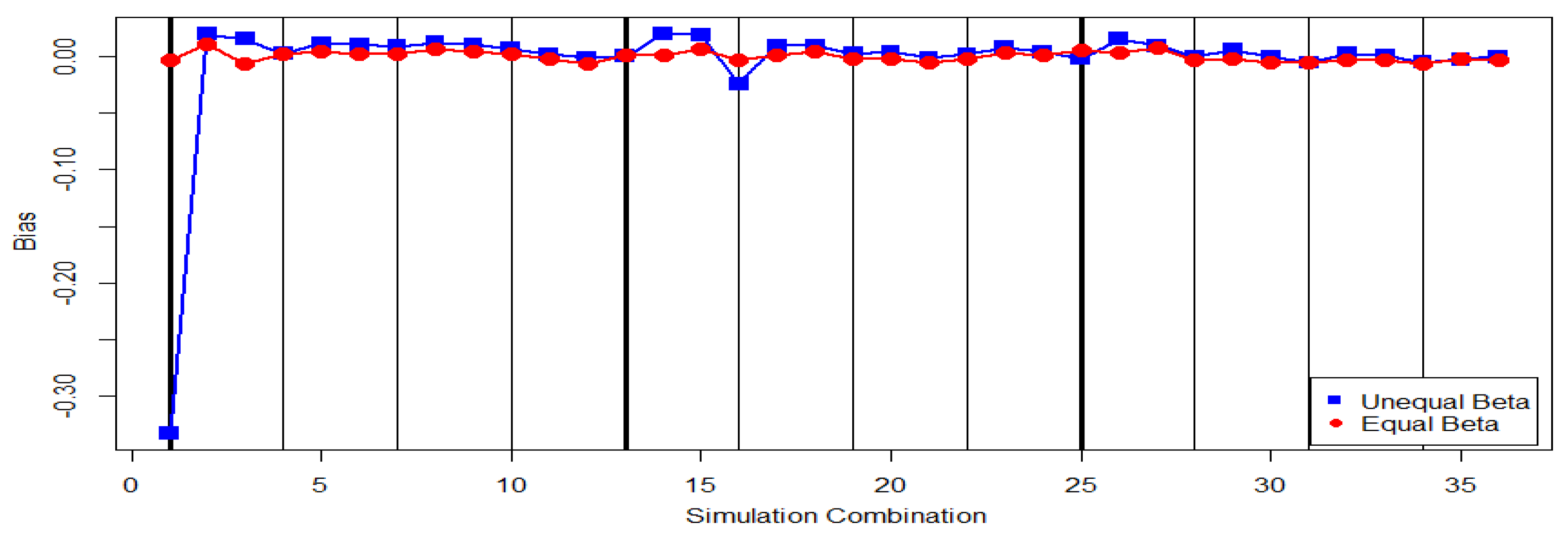
4.1. Bias
In the simulation study, the bias of estimator can be defined by
where
is the
ith Bayes estimate obtained from the
ith MCMC procedure under the SE loss function.
Table 1 contains the bias of
under each progressive first failure scheme for the case of
and
. From
Table 1, it can be seen that when
,
is more often to overestimate the true
. The bias of
in
Table 1 for the case of
is small. This means that the estimate
is more reliable for the case of
than that for the case of
.
Figure 1 also supports our findings from the simulation results of
Table 1. The bias of
for the case of
is closer to 0 with less fluctuation than the bias of
for the case of
.
The bias behaviors based on the estimates from and for estimating are similar to that based on the estimator . We only report the bias of to save space. In summary, the bias of these three Bayes estimators are small and the bias for the case of is smaller than the bias for the case of .
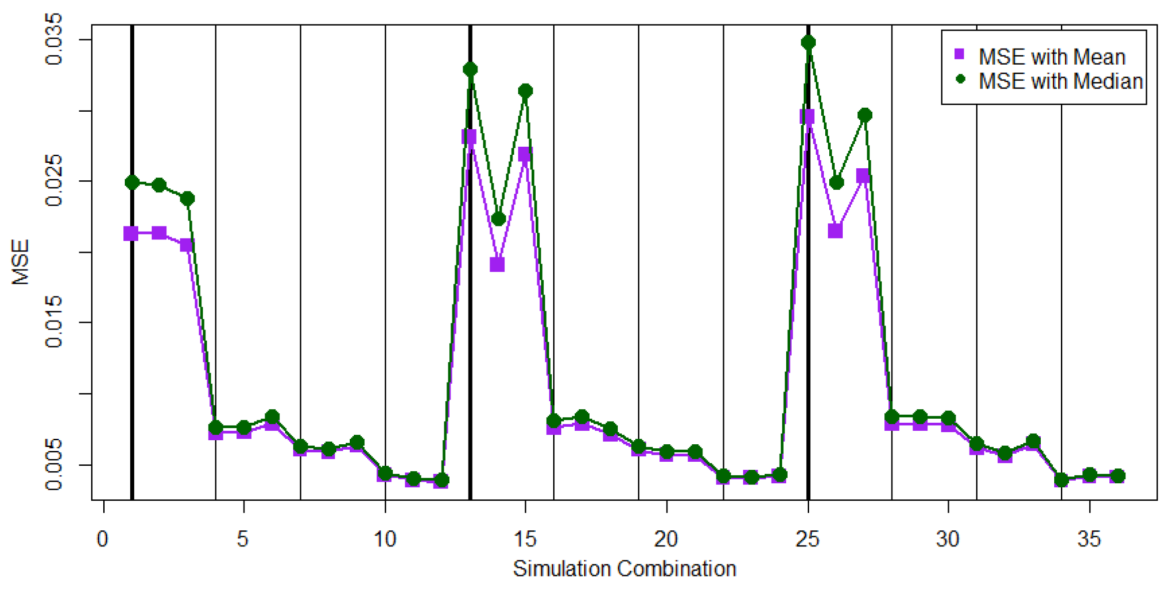
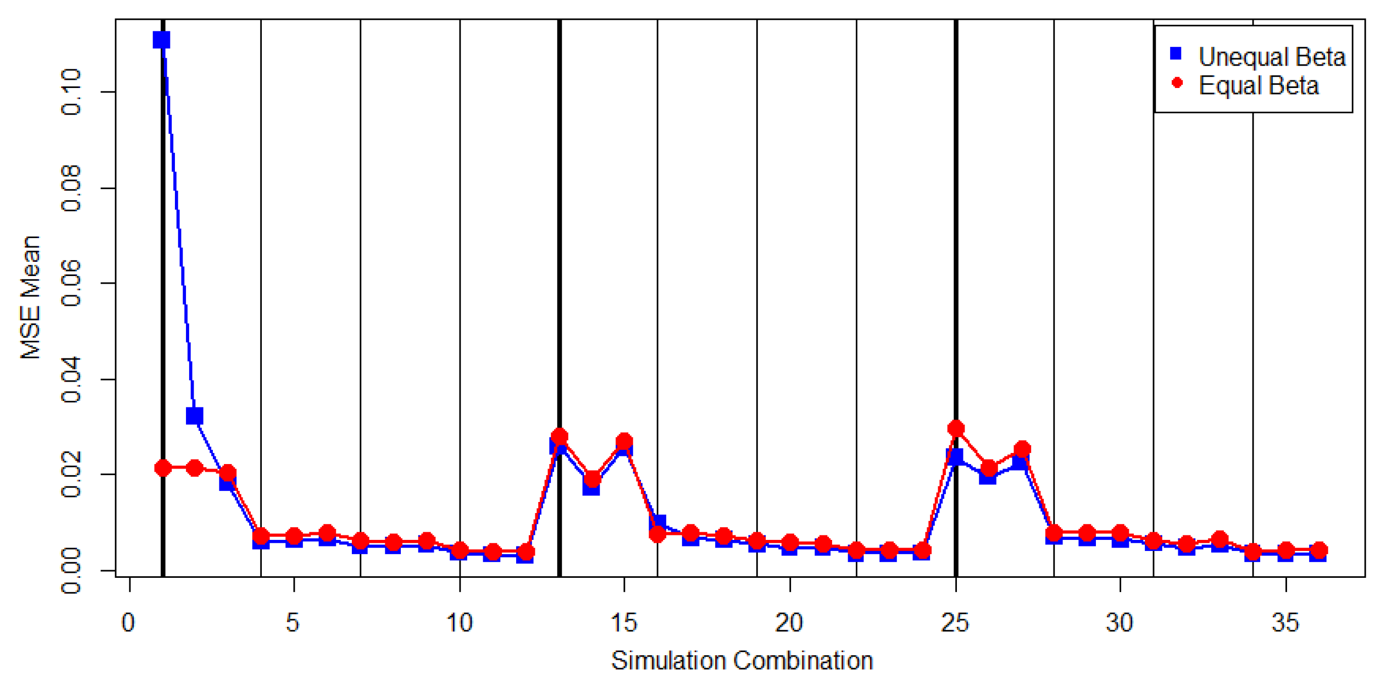
4.2. Expected Squared Error for and
To investigate the performance of using the estimator
and using
to estimate the true
, the ESE of the mean estimator,
and the ESE of the median estimator,
are evaluated. In this simulation study, the ESE of
and ESE of
can be defined, respectively, by
and
Table 2 contains the ESEs for using
and
to estimate
under each progressive first-failure censoring scheme. From
Table 2, we observe that most of the values of EAE (
) are smaller than the values of EAE (
) for two scenarios.
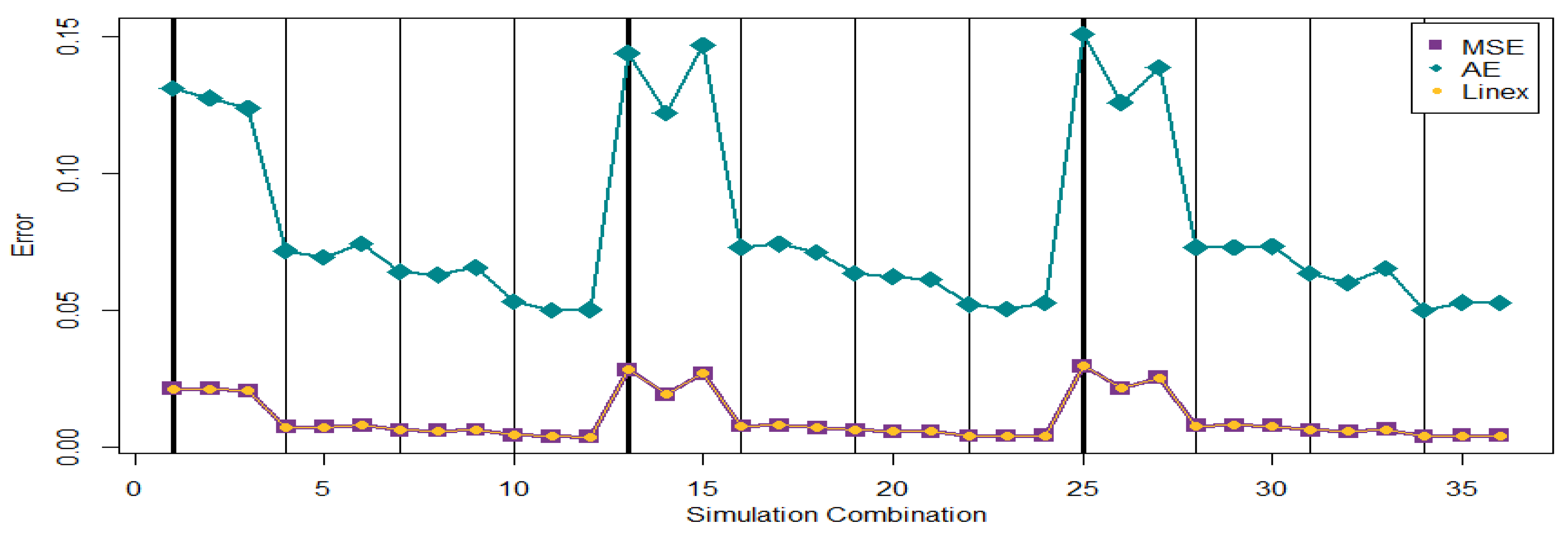
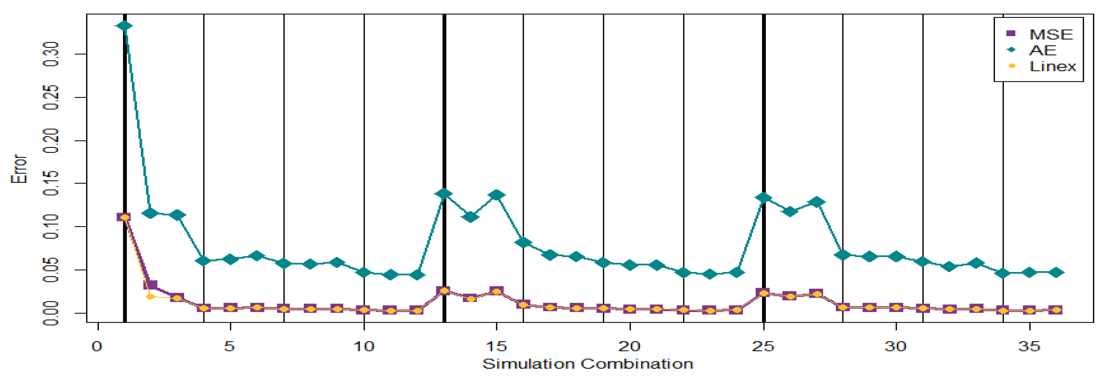
Figure 2 and
Figure 3 provide visual support.
For the case of , the values of EAE ( could be slightly larger than the values of EAE ( when the sample size is small. For the case of , performs better than with a smaller ESE.
We also compare the values of EAE (
between the cases of
and
.
Figure 4 displays the respective values of EAE (
at 36 parameter combinations for the cases of
and
.
From
Figure 4, we can find that the proposed MCMC method could generate a mild– large ESE when the sample size is small. The parameter combinations 1, 2, 3, 13, 14, 15, 25, 26, and 27 in
Figure 4 generate a mild–large ESE compared to that for the other parameter combinations. The simulation results in
Table 2 show that the progressive first failure-censoring scheme to remove survival units at the early stage can be a compromised design to generate a small ESE when using the proposed MCMC method with the SE loss function.
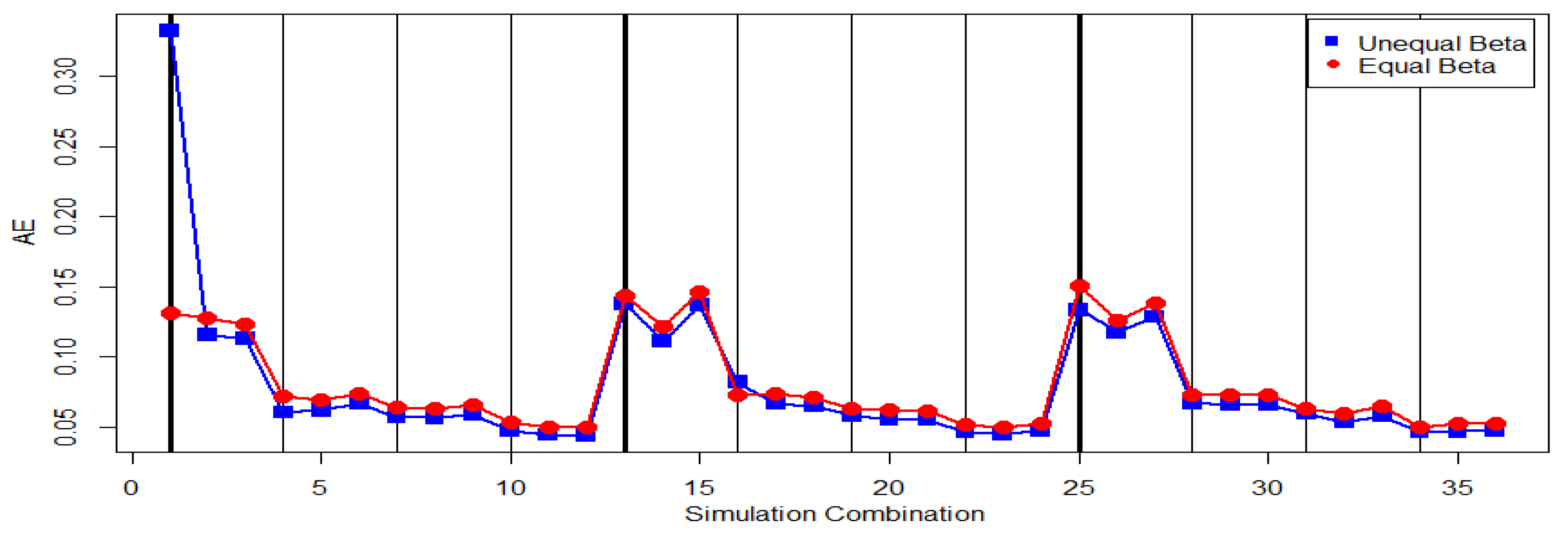
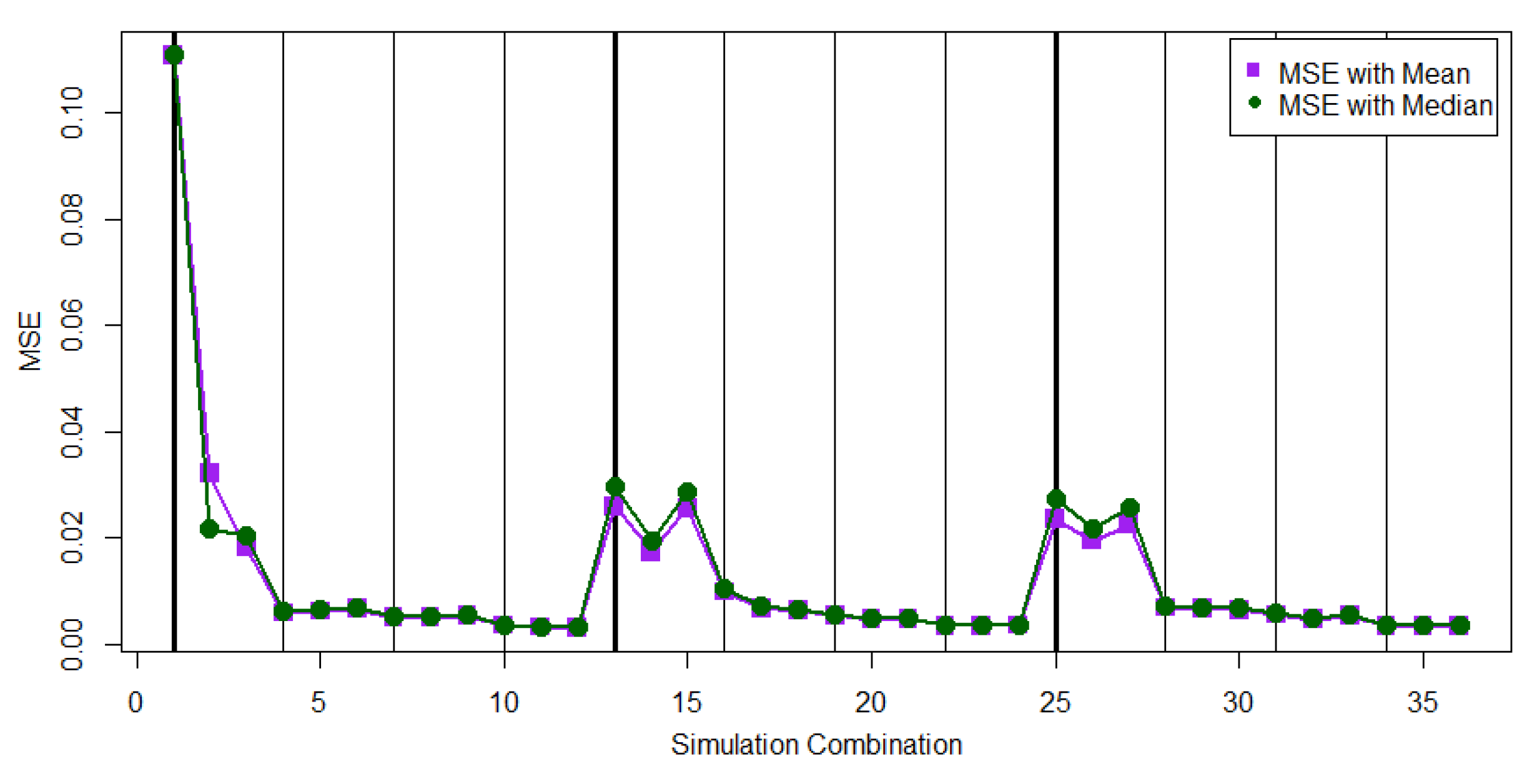
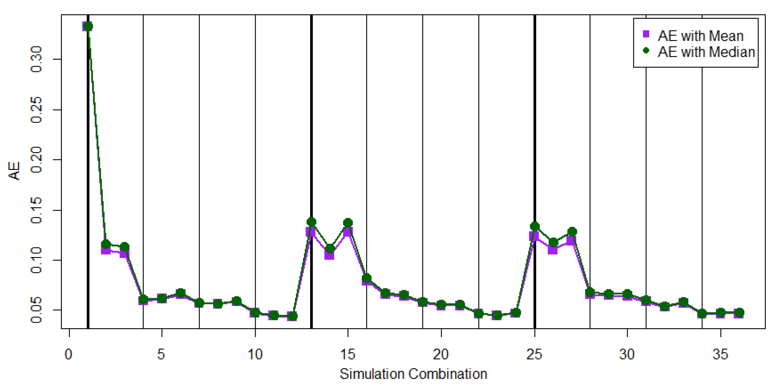
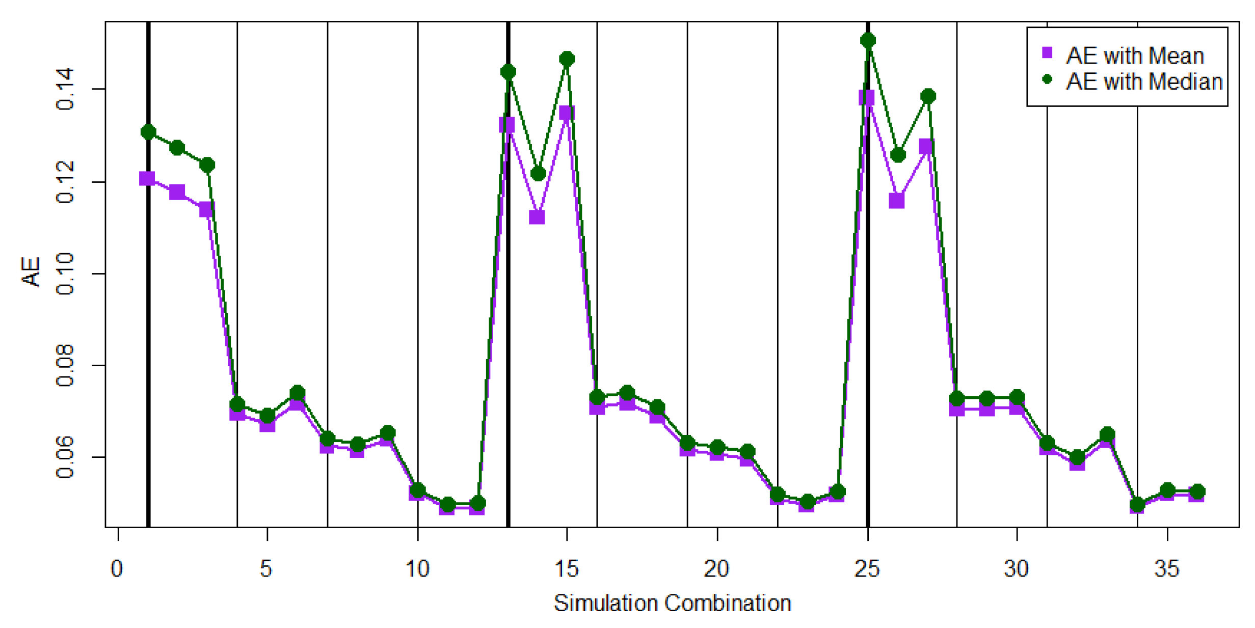
4.3. Expected Absolute Error for and
To investigate the performance of using the estimator
and of using the estimator
to estimate the true
, the EAE of the mean estimator,
, and the EAE of the median estimators,
, are evaluated. For the simulation study, the EAE (
) and EAE (
) are, respectively, defined by
and
Table 3 contains the EAEs of using
and
to estimate
for all progressive first failure schemes.
Figure 5 and
Figure 6 display the performance comparison, in terms of EAE, between using
and
to estimate
for the cases of
and
, respectively.
Table 3 shows that the value of EAE
is smaller than the value of EAE
for almost all 36 parameter combinations. When the sample size is small in the parameter combinations 1, 2, 3, 13, 14, 15, 25, 26, and 27, the proposed MCMC method with the AE loss function could generate large EAEs for both cases of
and
.
No dominant progressive first failure-censoring scheme can be found in
Table 3 in terms of small EAE values. We also compare the performance of
in terms of EAE under different cases of
and
.
Figure 7 displays the EAE values of using
to estimate
. From
Figure 7, we find that
for the case of
performs closely to that for the case of
except the first progressive first failure-censoring scheme.
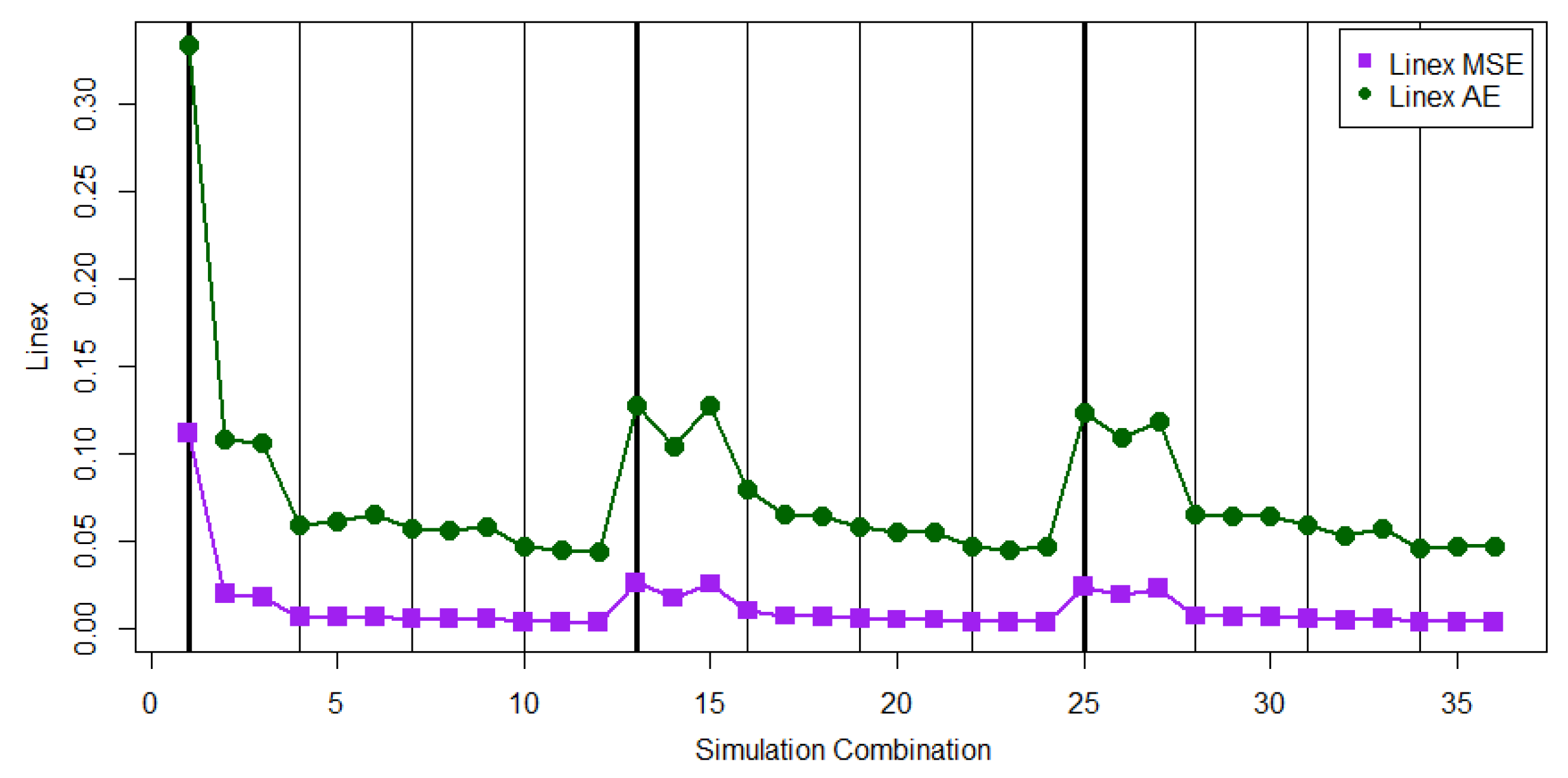
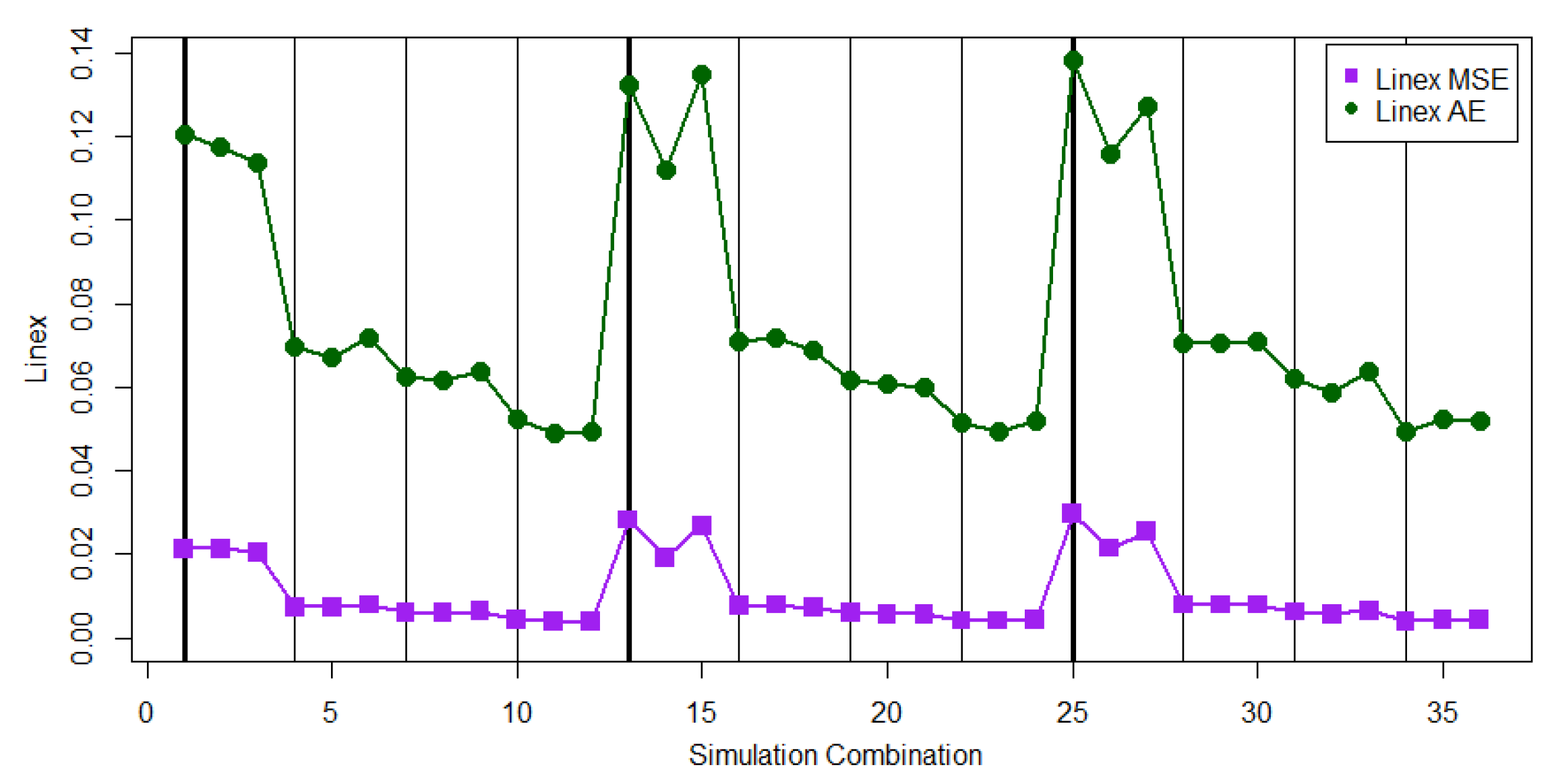
4.4. Expected Squared and Expected Absolute Errors for
In this subsection, the ESE and EAE of the Linex estimator
are evaluated to investigate the performance of using the estimator
to estimate the true
. For each simulation combination under the two scenarios, the EAE (
) and EAE (
) are, respectively, defined as
and
in which
is selected to obtain
.
Table 4 reports the ESE and EAE values based on using the Linex estimates for each progressive first failure-censoring scheme. The patterns of the ESE and EAE are displayed in
Figure 8 for the case of
and in
Figure 9 for the case of
.
In
Table 4, no dominant progressive first failure-censoring schemes with small ESE and EAE can be found. The EAE (
) and EAE (
) have similar patterns for both cases of
and
. The
cannot work well when the sample size is small.
Figure 8 and
Figure 9 show that the values of ESE and EAE for the parameter combinations 1, 2, 3, 13, 14, 15, 25, 26, and 27 are significantly larger than those for the other parameter combinations.
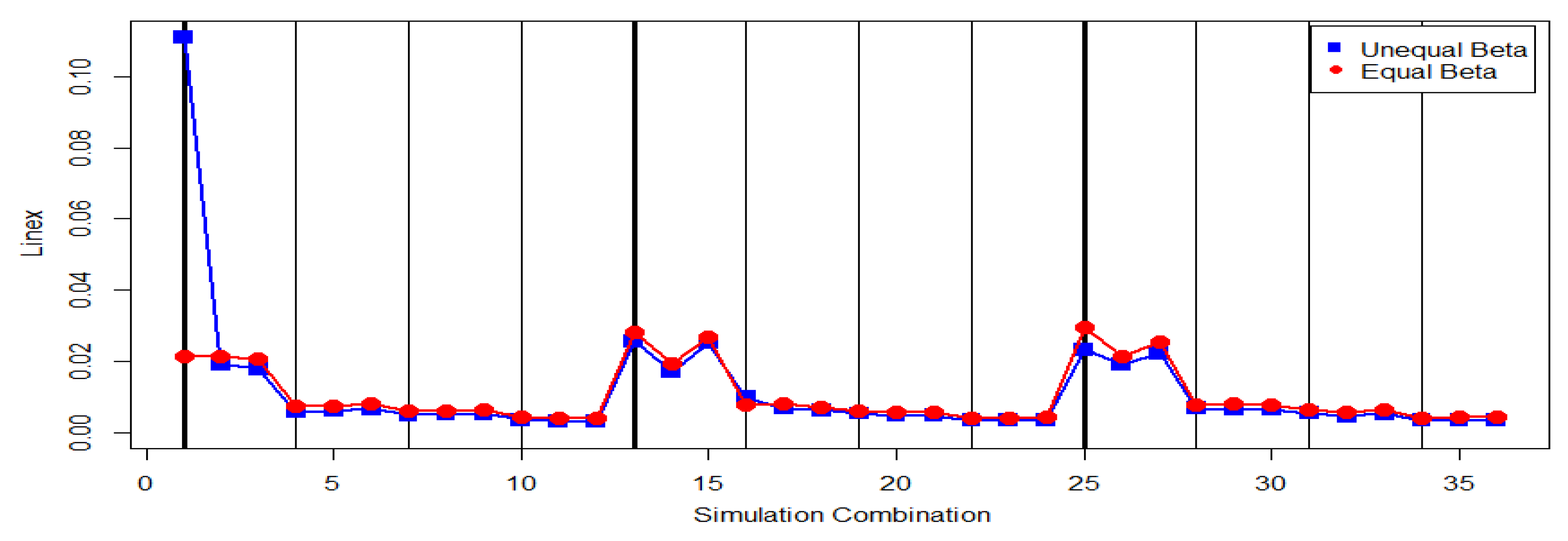
Figure 10 displays the values of EAE (
) for the cases of
and
. From
Figure 10, we can find that the values of EAE (
) are close for both cases of
and
for almost all 36 parameter combinations except for the first simulation parameter combination. This means that
has close performances under both cases.
4.5. Comparison between Expected Square Error on and and Expected Absolute Error on
Because the Bayes estimator based on the Linex loss function approaches the Bayes estimator based on the SE loss function as
, in this subsection, we want to understand the ESE behavior of
, the ESE behavior of
, and the EAE behavior of
. The values of the EAE (
), EAE (
), and EAE (
) are displayed in
Figure 11 and
Figure 12 for all 36 parameter combinations for the cases of
and
, respectively. Similar patterns are found in
Figure 11 and
Figure 12. From
Figure 11 and
Figure 12, it was noticed that the pattern of EAE (
) is oscillated more than the patterns of EAE (
) and EAE (
). All three Bayes estimators have larger evaluations for the ESE or EAE when the number of observed lifetimes is small. Moreover, the values of EAE (
) and EAE (
) are very close because
is used for the Linex loss function. It should be mentioned that ESE converges to the theoretical MSE, and EAE converges to the theoretical MAE when the number of MCMC iteration approaches infinity. Overall, the SE loss function can be a good option to find Bayes estimator. When the SE loss function is used to find Bayes estimator, the progressive first failure-censoring scheme with removing survival units at the early stage can be a compromised design to generate a small MSE. This property is helpful for practitioners to set up the progressive first failure-censoring scheme in practical applications.
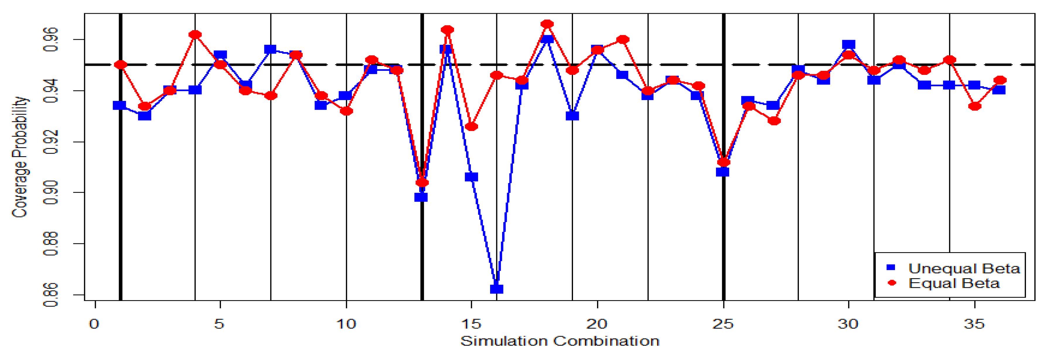
4.6. Evaluation of Credible Intervals
On the basis of the empirical distribution of
, a credible interval with the confidence level of
can be obtained from each MCMC procedure by taking two symmetric tail cuts as the lower and upper bounds, where
. These credible intervals provide a range of values, in which true
lies with a 95% level of confidence.
Table 5 reports the coverage probabilities of
to verify the performance of interval inference. All the coverage probabilities in
Table 5 are obtained via use of the relative frequency of the 500 simulated
credible intervals that cover the true
.
Figure 13 displays the pattern of the coverage probabilities in
Table 5. It can be noticed that most dots are plotted below the dash line of the nominal confidence level
. That is, most coverage probabilities underestimate the nominal confidence level. The credible interval inference method works more stably for the case of
than that for the case of
.
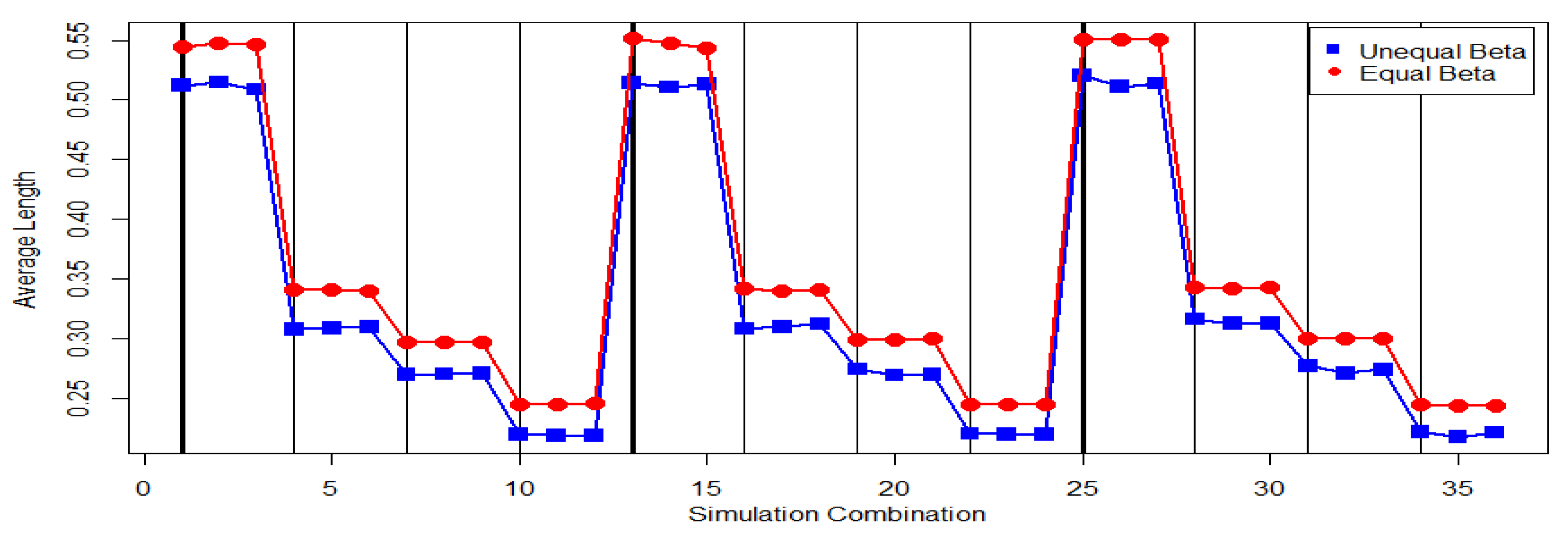
The average length of the credible interval can be determined from the simulated 500 credible intervals for each scenario. These results are displayed in
Table 5 and
Figure 14. From
Table 5, we find that the average length of the credible interval decreases as the sample size increases. It can also be observed from
Table 5 that different censoring schemes under both simulation scenarios have little impact on the average length of credible interval. However, the average length of credible intervals highly depends on the sample size.
Figure 14 shows the largest average length group occurring at the simulation parameter combinations with small sample sizes for
; see the simulation parameter combinations 1, 2, 3, 13, 14, 15, 25, 26, and 27.
Figure 14 also shows that the average lengths of credible intervals for the case of
are shorted than that for the case of
.
4.7. Performance Comparison between Bayesian Estimation and Maximum Likelihood Estimation Methods
The maximum likelihood estimation (MLE) method is another popular method for parameter estimation to search the maximizer of the likelihood function given a sample. In this subsection, the performance of the maximum likelihood estimation method and the Bayesian estimation method through bias and ESE will be investigated. Let
and
; the progressive first failure-censoring schemes
,
, and
are selected to implement the simulation study for comparing the performance of the maximum likelihood estimation method and the Bayesian estimation method. The bias and MSE are evaluated based on 10,000 MLEs and Bayes estimates of
, respectively, for the Burr type XII distribution with parameters
and
. All simulation results are reported in
Table 6 and
Table 7.
From
Table 6 and
Table 7, it can be noticed that the maximum likelihood estimation method and the proposed Bayesian estimation method are competitive. Both estimation methods can generate reliable estimates, which have small values of bias and ESE, for estimating
. On the basis of our simulation experience, we find that the convergence of the maximum likelihood estimation method could be a problem during maximizing the log-likelihood function to search the MLEs of the model parameters. The performance of the maximum likelihood estimation method highly depends on the initial solutions of the model parameters. It could be difficult for users to select good initial solutions in some situations. The proposed MCMC procedure using non-informative prior distributions can be applied to replace the maximum likelihood estimation method to generate Bayes estimates. When non-informative prior distributions are used, the resulting Bayes estimates are close to the MLEs, and then, the users can escape the convergence problem in numerical computation during maximization of the log-likelihood function. On the basis of this merit, the proposed MCMC procedure is recommended and can be an alternative of the maximum likelihood estimation method proposed by Lio and Tsai [
3].
5. Applications
The stress–strength parameter inference has earned widely discussions in reliability analysis applications. In this section, we firstly mention potential IoT applications in which can be used as an indicator to monitor the quality of IoT devices. Then, an example regarding the reliability of a component used in vehicles is used to illustrate the applications of methodologies proposed in this work.
5.1. IoT Applications
IoT devices have been widely applied in different areas, for example, smart cities. A smart city uses sensors to collect data for efficiently managing assets and resources. All the collected data are processed to monitor and manage important aspects such as the traffic and transportation systems, power projects, water supply networks, information systems, and different community services. The main strength of the IoT idea is the high impact it has on several aspects of everyday life and behavior of potential users. From the point of view of a private user, the most obvious effects of IoT introduction will be visible in both working and domestic fields. Comprehensive discussions about IoT applications for smart cities environments can be found in Atzori et al. [
26] and Tsiropoulou et al. [
27].
Dogmatics, assisted living, e-health, and enhanced learning are examples of possible application scenarios in which the new paradigm will play a leading role in the near future. The most apparent consequences will be equally visible in areas of logistics, process management, automation manufacturing, and intelligent transportation. On the basis of the aforementioned considerations, the US National Intelligence Council (NIC) includes the IoT in the list of six Disruptive Civil Technologies with potential impacts on US national power; see [
28]. NIC foresees that Internet nodes may reside in everyday things by 2025. Future opportunities will arise; for example, popular demands that combined with technology advances could drive widespread diffusion of the IoT. The possible threats deriving from a widespread adoption of IoT devices are also stressed. It is obvious that the threat deriving from a adoption of a technology is a stress indicator and the strength of the IoT devices is another important indicator. In such applications,
can be used to monitor the quality of each important IoT application and the proposed Bayes estimate can be used to estimate the stress–strength, providing that both stress and strength samples are available.
5.2. Reliability Evaluation for Vehicle Components
The next example is about the reliability evaluation for one type of component that is used in vehicles. The example can be found from Life Data Analysis Reference
http://reliawiki.org/index.php/Life_Data_Analysis_Reference_Book or from the link
http://reliawiki.org/index.php/Stress-Strength_Analysis. This example presents two data sets; the first data set is a random sample of size 20 from the usage mileage distribution per year as the stress, and the second data set is a random sample of size 50 from the miles-to-failure distribution as the strength for the component of which warranty is 1 year or 15,000 miles. Assuming that these two random samples have lognormal distributions, the given example used a different definition of stress–strength to calculate the point estimate of the stress–strength of the component by using these two random samples that withdrew vehicles with mileages larger than 15,000. Because the given random samples are not progressively first-failure censored samples, progressively first-failure censored samples from the same environment are generated to illustrate the application of the proposed methods.
First, we keep 20 observations from the first stress data set and randomly select 20 observations from the strength data set for Burr type XII modeling purposes. These two data sets in terms of 15,000 miles are displayed in
Table 8 for the Burr type XII modelings. Two Burr type XII distributions sharing the same inner shape parameter
are used to fit these two data sets shown in
Table 8 by using the likelihood function presented by Equation (
9) with
and both
R and
R equal to zero vectors for both stress and strength as random samples. The MLEs of
,
and
are obtained by
,
, and
. Followed by the Kolmogorov–Smirnov (KS) good-of-fit test for both Burr type XII distributions using MLEs as Burr type XII distribution parameters, the KS statistics based on the two data sets shown in
Table 8 are obtained as 0.2033 with the
p-value of 0.334 for the stress Burr type XII distribution model and as 0.2436 with the
p-value of 0.1573 for the strength Burr type XII distribution. The testing results from KS test indicate that the stress distribution can be well fitted by the Burr type XII distribution with
and that the strength distribution can be well fitted by the Burr type XII distribution with
. The true stress strength parameter is
.
A pair of progressively first failure-censored samples under
,
, and
and censored scheme
are generated from both stress Burr type XII
and the Burr type XII distribution with
three times, and the resulting three pairs are displayed in
Table 9. The prior distribution for
is the Gamma distribution with parameters
and
, the prior distribution for
is the Gamma distribution with parameters
and
, and the prior distribution for
is the Gamma distribution with parameters
and
. Each pair of progressively first failure-censored samples in
Table 9 will be used as the inputs to obtain a MCMC sample for
.
Figure 15 shows three time series plots, respectively, for the three
MCMC samples of
after burn-in. On the basis of the three MCMC samples after burn-in, by using the SE loss function, three Bayes estimates of
are obtained to be 0.8113, 0.8626, and 0.8475, respectively; by using the AE loss function, three Bayes estimates of
are obtained to be 0.8177, 0.8681, and 0.8551, respectively; and by using the Linex loss function, three Bayes estimates of
are obtained to be 0.8104, 0.8619, and 0.8467, respectively. Moreover, three
credible intervals of
based on the three
MCMC samples after burn-in are given as
,
, and
, respectively. It seems that these three Bayes estimates are not as accurate as expected. It could be the true stress–strength parameter
close to one of theoretical boundaries that is 1.0 in this application. This is commonly known as the boundary effect which is worth further investigating.
6. Conclusions
Bayesian inferences of the stress–strength parameter in a system of two components are investigated based on a pair of progressively first failure-censored samples from two independent Burr type XII distributions, which share a common inner shape parameter. Because of the lack of closed forms for the conditional posterior distributions and the difficulties of computation complexities, a MCMC procedure to implement the M–H algorithm via Gibbs sampling is established to collect samples from the posterior distribution of .
The SE, AE, and Linex loss functions are used to search the Bayes estimates of the model parameters. An intensive simulation study has been conducted to show that the SE loss function can be a good option to implement the proposed estimation method with a progressive first failure-censoring scheme, in which survival units were removed in the early stage. These findings provide a good suggestion for users to select a progressive first failure-censoring scheme for the practical application. The proposed estimation method needs a sample size of at least 30 to obtain a reliable Bayes estimate for the stress–strength parameter. The coverage probability and its average length of the credible interval for the stress–strength parameter were also investigated. Simulation results show that our proposed estimation methods work well when true stress–strength not near the boundary (0 or 1.0). The Bayes estimate of the stress–strength parameter based on progressively first failure-censored samples would be a good future investigation when the true stress–strength parameter is very close to 0 or 1.
The effectiveness of some progressive first failure-censoring schemes to the Bayes estimators is investigated through Monte Carol simulations. Moreover, the estimation performance of the proposed estimation method is compared with the maximum likelihood estimation method using simulations. We find that the proposed estimation method and maximum likelihood estimation method are competitive in generating reliable estimates of the model parameters with small bias and MSE. We also found that the convergence of the maximum likelihood estimation method could be a problem during maximizing the log-likelihood function to search the MLEs of model parameters. It could be difficult for users to set up good initial solutions in some situations to search MLEs. The proposed MCMC procedure using non-informative prior distributions can be applied to replace the maximum likelihood estimation method to generate Bayes estimates, which are close to the MLEs. The proposed MCMC procedure is hence recommended to be an alternative of the maximum likelihood estimation method. More and more IoT devices are used to establish smart city environments. Nowadays, the inference of the stress–strength parameter with complete big data becomes an important topic for monitoring the quality of IoT devices over time. This topic is interesting and will be studied in the near future.
Author Contributions
Conceptualization, Y.L.; methodology, Y.L., T.-R.T.; software, Y.-J.L.; validation, J.M.B., Y.-J.L. and Y.L.; formal analysis, Y.L., J.M.B., T.-R.T.; investigation, Y.L., T.-R.T., J.M.B., Y.-J.L.; resources, Y.L., T.-R.T., J.M.B., Y.-J.L.; data curation, Y.L., T.-R.T., Y.-J.L.; writing–original draft preparation, Y.L., J.M.B.; writing–review and editing, Y.L., T.-R.T.; visualization, Y.L., T.-R.T.; supervision, Y.L., T.-R.T., Y.-J.L.; project administration, Y.L., T.-R.T., Y.-J.L.; funding acquisition, T.-R.T.
Funding
This study is supported by the grant of Ministry of Science and Technology, Taiwan MOST 108-2221-E-032-018-MY2.
Acknowledgments
The authors would also like to thank for the suggestions from reviewers to improve the paper significantly.
Conflicts of Interest
The authors declare no conflict of interest.
References
- Balakrishnan, N.; Aggarwala, R. Progressive Censoring: Theory, Methods and Applications; Birkhauser: Boston, MA, USA, 2000. [Google Scholar]
- Balasooriya, U. Failure-censored reliability sampling plans for the exponential distribution. J. Stat. Comput. Simul. 1995, 52, 337–349. [Google Scholar] [CrossRef]
- Lio, Y.L.; Tsai, T.-R. Estimation of δ = P(X < Y) for Burr XII distribution based on the progressively first failure-censored samples. J. Appl. Stat. 2012, 39, 309–322. [Google Scholar]
- Wu, S.; Kuş, C. On estimation based on progressive first-failure-censored sampling. Comput. Stat. Data Anal. 2009, 53, 3659–3670. [Google Scholar] [CrossRef]
- Birnbaum, Z.W. On a use of Mann-Whitney statistics. In Proceedings of the Third Berkley Symposium in Mathematics, Statistics and Probability; University of California Press: Berkeley, CA, USA, 1956; Volume 1, pp. 13–17. [Google Scholar]
- Tong, H. A note on the estimation of P(Y < X) in the exponential case. Technometrics 1974, 16, 625. [Google Scholar]
- Surles, J.G.; Padgett, W.J. Inference for P(Y < X) in the Burr type X model. J. Appl. Stat. Sci. 1998, 7, 225–238. [Google Scholar]
- Kundu, D.; Gupta, R.D. Estimation of R = P(Y < X) for the generalized exponential distribution. Metrika 2005, 61, 291–308. [Google Scholar]
- Kundu, D.; Gupta, R.D. Estimation of R = P(Y < X) for Weibull distribution. IEEE Trans. Reliab. 2006, 55, 270–280. [Google Scholar]
- Raqab, M.Z.; Madi, M.T.; Kundu, D. Estimation of R = P(Y < X) for the 3-parameter generalized exponential distribution. Commun. Stat. Theor. Methods 2008, 37, 2854–2864. [Google Scholar]
- Kim, C.; Chung, Y. Bayesian estimation of P(Y < X) from Burr type X model containing spurious observations. Stat. Pap. 2006, 47, 643–651. [Google Scholar]
- Kundu, D.; Raqab, M.Z. Estimation of R = P(Y < X) for three parameter Weibull distribution. Stat. Probabil. Lett. 2009, 79, 1839–1846. [Google Scholar]
- Kotz, S.; Lumelskii, Y.; Pensky, M. The Stress-strength Model and Its Generalization: Theory and Applications; World Scientific: Singapore, 2003. [Google Scholar]
- Saracoglu, B.; Kaya, M.F. Maximum likelihood estimation and confidence intervals of system reliability for Gompertz distribution in stress-strength models. Seluk J. Appl. Math. 2007, 8, 25–36. [Google Scholar]
- Saracoglu, B.; Kaya, M.F.; Abd-Elfattah, A.M. Comparison of estimators for stress-strength reliability in Gompertz case. Hacettepe J. Math. Stat. 2009, 38, 339–349. [Google Scholar]
- Jiang, L.; Wong, A.C.M. A note on inference for P(X < Y) for right truncated exponentially distribution data. Stat. Pap. 2008, 49, 637–651. [Google Scholar]
- Saracoglu, B.; Kuş, C. Estimation of the stress-strength reliability under progressive censoring for Gompertz distribution. In Proceedings of the Sixth Symposium of Statistics Days; OndokuzMayis University: Samsun, Turkey, 2008; pp. 464–471. [Google Scholar]
- Saracoglu, B.; Kinaci, I.; Kundu, D. On estimation of R = P(Y < X) for exponential distribution under progressive type-II censoring. J. Stat. Comput. Simul. 2012, 82, 729–744. [Google Scholar]
- Burr, I.W. Cumulative frequency functions. Ann. Math. Stat. 1942, 13, 215–232. [Google Scholar] [CrossRef]
- Metropolis, N.; Rosenbluth, A.W.; Rosenbluth, M.N.; Teller, A.H.; Teller, E. Equations of state calculations by fast computational machine. J. Chem. Phys. 1953, 21, 1087–1091. [Google Scholar] [CrossRef]
- Hastings, W.K. Monte Carlo Sampling Methods Using Markov Chains and Their Applications. Biometrika 1970, 57, 97–109. [Google Scholar] [CrossRef]
- Geman, S.; Geman, D. Stochastic relaxation, Gibbs distribution and the Bayesian restoration of images. IEEE Trans. Pattern Anal. 1984, 6, 721–741. [Google Scholar] [CrossRef]
- Panahi, H.; Sayyareh, A. Parameter estimation and prediction of order statistics for the Burr type XII distribution with type II censoring. J. Appl. Stat. 2014, 41, 215–232. [Google Scholar] [CrossRef]
- Lin, Y.-J.; Lio, Y.L.; Ng, H.K.T. Bayes estimation of Moran-Downton bivariate exponential distribution based on censored samples. J. Stat. Comput. Simul. 2013, 83, 837–852. [Google Scholar] [CrossRef]
- Lunn, D.; Jackson, C.; Best, N.; Thomas, A.; Spiegelhalter, D. The BUGS Book: A Practical Introduction to Bayesian Analysis; CRC Press: New York, NY, USA; Taylor & Fransis Group: Abingdon, UK, 2012; pp. 204–205. [Google Scholar]
- Atzori, L.; Iera, A.; Morabito, G. The Internet of Things: A survey. Comput. Netw. 2010, 54, 2787–2805. [Google Scholar] [CrossRef]
- Tsiropoulou, E.E.; Baras, J.S.; Papavassiliou, S.; Sinha, S. RFID-based smart parking management system. Cyber-Phys. Syst. 2017, 3, 22–41. [Google Scholar] [CrossRef]
- National Intelligence Council. Disruptive Civil Technologies: Six Technologies with Potential Impacts on US Interests Out to 2025—Conference Report CR 2008–07; National Intelligence Council: Washington, DC, USA, 2008. [Google Scholar]
Figure 1.
The bias of for the cases of and .
Figure 1.
The bias of for the cases of and .
Figure 2.
The expected square errors (ESEs) of and for the case of .
Figure 2.
The expected square errors (ESEs) of and for the case of .
Figure 3.
The ESEs of and for the case of .
Figure 3.
The ESEs of and for the case of .
Figure 4.
The value of expected absolute error (EAE; for the cases of and .
Figure 4.
The value of expected absolute error (EAE; for the cases of and .
Figure 5.
The EAEs of and for the case of .
Figure 5.
The EAEs of and for the case of .
Figure 6.
The EAEs of and for the case of .
Figure 6.
The EAEs of and for the case of .
Figure 7.
The values of EAE for the cases of and .
Figure 7.
The values of EAE for the cases of and .
Figure 8.
The values of EAE () and EAE () for the case of .
Figure 8.
The values of EAE () and EAE () for the case of .
Figure 9.
The values of EAE () and EAE () for the case of .
Figure 9.
The values of EAE () and EAE () for the case of .
Figure 10.
The values of EAE () for the cases of and .
Figure 10.
The values of EAE () for the cases of and .
Figure 11.
Overall error under .
Figure 11.
Overall error under .
Figure 12.
Overall error under .
Figure 12.
Overall error under .
Figure 13.
Comparison of coverage probabilities
Figure 13.
Comparison of coverage probabilities
Figure 14.
Average length of covering confidence intervals
Figure 14.
Average length of covering confidence intervals
Figure 15.
Comparison of coverage probabilities.
Figure 15.
Comparison of coverage probabilities.
Table 1.
The bias of under different Burr type XII distributions.
Table 1.
The bias of under different Burr type XII distributions.
| | Parameter Combinations | Simulation Scenarios |
|---|
| | | | | Scheme | | |
|---|
| 1 | 1 | 20 | 5 | (0, 0, 0, 0, 15) | −0.3326 | −0.0032 |
| 2 | | | | (15, 0, 0, 0, 0) | 0.0196 | 0.0112 |
| 3 | | | | (3, 3, 3, 3, 3) | 0.0155 | −0.0062 |
| 4 | | 30 | 15 | (0, …, 0, 15) | 0.0025 | 0.0020 |
| 5 | | | | (15, 0, …, 0) | 0.0113 | 0.0037 |
| 6 | | | | (3, 0, 0, …, 3, 0, 0) | 0.0102 | 0.0015 |
| 7 | | 50 | 20 | (0, …, 0, 30) | 0.0089 | 0.0018 |
| 8 | | | | (30, 0, …, 0) | 0.0122 | 0.0062 |
| 9 | | | | (3, 0, 3, 0, …, 3, 0) | 0.0103 | 0.0038 |
| 10 | | | 30 | (0, …, 0, 20) | 0.0066 | 0.0017 |
| 11 | | | | (20, 0, …, 0) | 0.0018 | −0.0028 |
| 12 | | | | (2, 0, 0, …, 2, 0, 0) | −0.0013 | −0.0065 |
| 13 | 3 | 20 | 5 | (0, 0, 0, 0, 15) | <0.0001 | 0.0009 |
| 14 | | | | (15, 0, 0, 0, 0) | 0.0201 | 0.0012 |
| 15 | | | | (3, 3, 3, 3, 3) | 0.0192 | 0.0062 |
| 16 | | 30 | 15 | (0, …, 0, 15) | −0.0244 | −0.0033 |
| 17 | | | | (15, 0, …, 0) | 0.0093 | 0.0015 |
| 18 | | | | (3, 0, 0, …, 3, 0, 0) | 0.0096 | 0.0037 |
| 19 | | 50 | 20 | (0, …, 0, 30) | 0.0024 | −0.0026 |
| 20 | | | | (30, 0, …, 0) | 0.0040 | −0.0020 |
| 21 | | | | (3, 0, 3, 0, …, 3, 0) | −0.0013 | −0.0054 |
| 22 | | | 30 | (0, …, 0, 20) | 0.0020 | −0.0027 |
| 23 | | | | (20, 0, …, 0) | 0.0076 | 0.0035 |
| 24 | | | | (2, 0, 0, …, 2, 0, 0) | 0.0039 | 0.0007 |
| 25 | 5 | 20 | 5 | (0, 0, 0, 0, 15) | −0.0021 | 0.0052 |
| 26 | | | | (15, 0, 0, 0, 0) | 0.0153 | 0.0028 |
| 27 | | | | (3, 3, 3, 3, 3) | 0.0092 | 0.0071 |
| 28 | | 30 | 15 | (0, …, 0, 15) | −0.0003 | −0.0037 |
| 29 | | | | (15, 0, …, 0) | 0.0058 | −0.0019 |
| 30 | | | | (3, 0, 0, …, 3, 0, 0) | −0.0003 | −0.0060 |
| 31 | | 50 | 20 | (0, …, 0, 30) | −0.0055 | −0.0053 |
| 32 | | | | (30, 0, …, 0) | 0.0022 | −0.0034 |
| 33 | | | | (3, 0, 3, 0, …, 3, 0) | 0.0006 | −0.0031 |
| 34 | | | 30 | (0, …, 0, 20) | −0.0054 | −0.0071 |
| 35 | | | | (20, 0, …, 0) | −0.0024 | −0.0019 |
| 36 | | | | (2, 0, 0, …, 2, 0, 0) | −0.0002 | −0.0038 |
Table 2.
The ESEs for and under two different Burr type XII distributions.
Table 2.
The ESEs for and under two different Burr type XII distributions.
| | Parameter Combinations | Simulation Scenarios |
|---|
| | | | | | | |
|---|
| | | | | Scheme | EAE () | EAE () | EAE () | EAE () |
|---|
| 1 | 1 | 20 | 5 | (0, 0, 0, 0, 15) | 0.1109 | 0.1109 | 0.0213 | 0.1205 |
| 2 | | | | (15, 0, 0, 0, 0) | 0.0321 | 0.0216 | 0.0213 | 0.1176 |
| 3 | | | | (3, 3, 3, 3, 3) | 0.0181 | 0.0203 | 0.0205 | 0.1137 |
| 4 | | 30 | 15 | (0, …, 0, 15) | 0.0058 | 0.0061 | 0.0072 | 0.0696 |
| 5 | | | | (15, 0, …, 0) | 0.0062 | 0.0063 | 0.0072 | 0.0672 |
| 6 | | | | (3, 0, 0, …, 3, 0, 0) | 0.0066 | 0.0068 | 0.0079 | 0.0719 |
| 7 | | 50 | 20 | (0, …, 0, 30) | 0.0049 | 0.0051 | 0.0061 | 0.0626 |
| 8 | | | | (30, 0, …, 0) | 0.0050 | 0.0051 | 0.0059 | 0.0616 |
| 9 | | | | (3, 0, 3, 0, …, 3, 0) | 0.0053 | 0.0054 | 0.0063 | 0.0640 |
| 10 | | | 30 | (0, …, 0, 20) | 0.0035 | 0.0036 | 0.0043 | 0.0523 |
| 11 | | | | (20, 0, …, 0) | 0.0032 | 0.0032 | 0.0039 | 0.0491 |
| 12 | | | | (2, 0, 0, …, 2, 0, 0) | 0.0030 | 0.0031 | 0.0038 | 0.0492 |
| 13 | 3 | 20 | 5 | (0, 0, 0, 0, 15) | 0.0259 | 0.0298 | 0.0281 | 0.1322 |
| 14 | | | | (15, 0, 0, 0, 0) | 0.0173 | 0.0193 | 0.0191 | 0.1121 |
| 15 | | | | (3, 3, 3, 3, 3) | 0.0255 | 0.0288 | 0.0269 | 0.1348 |
| 16 | | 30 | 15 | (0, …, 0, 15) | 0.0098 | 0.0105 | 0.0076 | 0.0709 |
| 17 | | | | (15, 0, …, 0) | 0.0067 | 0.0070 | 0.0079 | 0.0718 |
| 18 | | | | (3, 0, 0, …, 3, 0, 0) | 0.0062 | 0.0065 | 0.0071 | 0.0689 |
| 19 | | 50 | 20 | (0, …, 0, 30) | 0.0053 | 0.0055 | 0.0061 | 0.0619 |
| 20 | | | | (30, 0, …, 0) | 0.0046 | 0.0048 | 0.0057 | 0.0608 |
| 21 | | | | (3, 0, 3, 0, …, 3, 0) | 0.0047 | 0.0049 | 0.0056 | 0.0597 |
| 22 | | | 30 | (0, …, 0, 20) | 0.0033 | 0.0035 | 0.0041 | 0.0512 |
| 23 | | | | (20, 0, …, 0) | 0.0033 | 0.0034 | 0.0040 | 0.0496 |
| 24 | | | | (2, 0, 0, …, 2, 0, 0) | 0.0035 | 0.0036 | 0.0042 | 0.0519 |
| 25 | 5 | 20 | 5 | (0, 0, 0, 0, 15) | 0.0235 | 0.0272 | 0.0296 | 0.1382 |
| 26 | | | | (15, 0, 0, 0, 0) | 0.0194 | 0.0218 | 0.0215 | 0.1157 |
| 27 | | | | (3, 3, 3, 3, 3) | 0.0225 | 0.0258 | 0.0254 | 0.1274 |
| 28 | | 30 | 15 | (0, …, 0, 15) | 0.0068 | 0.0072 | 0.0078 | 0.0705 |
| 29 | | | | (15, 0, …, 0) | 0.0065 | 0.0068 | 0.0079 | 0.0706 |
| 30 | | | | (3, 0, 0, …, 3, 0, 0) | 0.0064 | 0.0067 | 0.0078 | 0.0709 |
| 31 | | 50 | 20 | (0, …, 0, 30) | 0.0054 | 0.0057 | 0.0062 | 0.0620 |
| 32 | | | | (30, 0, …, 0) | 0.0045 | 0.0047 | 0.0056 | 0.0587 |
| 33 | | | | (3, 0, 3, 0, …, 3, 0) | 0.0052 | 0.0054 | 0.0064 | 0.0638 |
| 34 | | | 30 | (0, …, 0, 20) | 0.0033 | 0.0034 | 0.0038 | 0.0492 |
| 35 | | | | (20, 0, …, 0) | 0.0033 | 0.0034 | 0.0042 | 0.0521 |
| 36 | | | | (2, 0, 0, …, 2, 0, 0) | 0.0034 | 0.0035 | 0.0041 | 0.0518 |
Table 3.
The EAEs for and under two different Burr type XII distributions.
Table 3.
The EAEs for and under two different Burr type XII distributions.
| | Parameter Combinations | Simulation Scenarios |
|---|
| | | | | | | |
|---|
| | | | | Scheme | EAE () | EAE () | EAE () | EAE () |
|---|
| 1 | 1 | 20 | 5 | (0, 0, 0, 0, 15) | 0.3328 | 0.3327 | 0.1205 | 0.1309 |
| 2 | | | | (15, 0, 0, 0, 0) | 0.1096 | 0.1157 | 0.1176 | 0.1275 |
| 3 | | | | (3, 3, 3, 3, 3) | 0.1066 | 0.1133 | 0.1137 | 0.1235 |
| 4 | | 30 | 15 | (0, …, 0, 15) | 0.0592 | 0.0607 | 0.0696 | 0.0717 |
| 5 | | | | (15, 0, …, 0) | 0.0611 | 0.0622 | 0.0672 | 0.0692 |
| 6 | | | | (3, 0, 0, …, 3, 0, 0) | 0.0657 | 0.0668 | 0.0719 | 0.0741 |
| 7 | | 50 | 20 | (0, …, 0, 30) | 0.0565 | 0.0574 | 0.0626 | 0.0640 |
| 8 | | | | (30, 0, …, 0) | 0.0562 | 0.0568 | 0.0616 | 0.0628 |
| 9 | | | | (3, 0, 3, 0, …, 3, 0) | 0.0583 | 0.0591 | 0.0640 | 0.0655 |
| 10 | | | 30 | (0, …, 0, 20) | 0.0471 | 0.0475 | 0.0523 | 0.0531 |
| 11 | | | | (20, 0, …, 0) | 0.0442 | 0.0448 | 0.0491 | 0.0498 |
| 12 | | | | (2, 0, 0, …, 2, 0, 0) | 0.0436 | 0.0442 | 0.0492 | 0.0501 |
| 13 | 3 | 20 | 5 | (0, 0, 0, 0, 15) | 0.1275 | 0.1382 | 0.1322 | 0.1437 |
| 14 | | | | (15, 0, 0, 0, 0) | 0.1044 | 0.1114 | 0.1121 | 0.1219 |
| 15 | | | | (3, 3, 3, 3, 3) | 0.1280 | 0.1370 | 0.1348 | 0.1465 |
| 16 | | 30 | 15 | (0, …, 0, 15) | 0.0793 | 0.0822 | 0.0709 | 0.0731 |
| 17 | | | | (15, 0, …, 0) | 0.0657 | 0.0672 | 0.0718 | 0.0741 |
| 18 | | | | (3, 0, 0, …, 3, 0, 0) | 0.0640 | 0.0654 | 0.0689 | 0.0710 |
| 19 | | 50 | 20 | (0, …, 0, 30) | 0.0574 | 0.0585 | 0.0619 | 0.0633 |
| 20 | | | | (30, 0, …, 0) | 0.0546 | 0.0556 | 0.0608 | 0.0623 |
| 21 | | | | (3, 0, 3, 0, …, 3, 0) | 0.0544 | 0.0555 | 0.0597 | 0.0612 |
| 22 | | | 30 | (0, …, 0, 20) | 0.0463 | 0.0469 | 0.0512 | 0.0520 |
| 23 | | | | (20, 0, …, 0) | 0.0448 | 0.0452 | 0.0496 | 0.0504 |
| 24 | | | | (2, 0, 0, …, 2, 0, 0) | 0.0468 | 0.0474 | 0.0519 | 0.0527 |
| 25 | 5 | 20 | 5 | (0, 0, 0, 0, 15) | 0.1234 | 0.1337 | 0.1382 | 0.1506 |
| 26 | | | | (15, 0, 0, 0, 0) | 0.1103 | 0.1177 | 0.1157 | 0.1257 |
| 27 | | | | (3, 3, 3, 3, 3) | 0.1191 | 0.1287 | 0.1274 | 0.1386 |
| 28 | | 30 | 15 | (0, …, 0, 15) | 0.0656 | 0.0676 | 0.0705 | 0.0728 |
| 29 | | | | (15, 0, …, 0) | 0.0645 | 0.0659 | 0.0706 | 0.0728 |
| 30 | | | | (3, 0, 0, …, 3, 0, 0) | 0.0639 | 0.0659 | 0.0709 | 0.0732 |
| 31 | | 50 | 20 | (0, …, 0, 30) | 0.0584 | 0.0600 | 0.0620 | 0.0634 |
| 32 | | | | (30, 0, …, 0) | 0.0530 | 0.0539 | 0.0587 | 0.0600 |
| 33 | | | | (3, 0, 3, 0, …, 3, 0) | 0.0571 | 0.0583 | 0.0638 | 0.0653 |
| 34 | | | 30 | (0, …, 0, 20) | 0.0458 | 0.0465 | 0.0492 | 0.0499 |
| 35 | | | | (20, 0, …, 0) | 0.0466 | 0.0472 | 0.0521 | 0.0528 |
| 36 | | | | (2, 0, 0, …, 2, 0, 0) | 0.0466 | 0.0473 | 0.0518 | 0.0525 |
Table 4.
The ESE and EAE for under different Burr type XII distributions.
Table 4.
The ESE and EAE for under different Burr type XII distributions.
| | Parameter Combinations | Simulation Scenarios |
|---|
| | | | | | | |
|---|
| | | | | Scheme | EAE () | EAE () | EAE () | EAE () |
|---|
| 1 | 1 | 20 | 5 | (0, 0, 0, 0, 15) | 0.1111 | 0.3333 | 0.0213 | 0.1205 |
| 2 | | | | (15, 0, 0, 0, 0) | 0.0191 | 0.1082 | 0.0212 | 0.1174 |
| 3 | | | | (3, 3, 3, 3, 3) | 0.0177 | 0.1054 | 0.0205 | 0.1139 |
| 4 | | 30 | 15 | (0, …, 0, 15) | 0.0058 | 0.0590 | 0.0072 | 0.0696 |
| 5 | | | | (15, 0, …, 0) | 0.0061 | 0.0608 | 0.0072 | 0.0672 |
| 6 | | | | (3, 0, 0, …, 3, 0, 0) | 0.0066 | 0.0653 | 0.0079 | 0.0718 |
| 7 | | 50 | 20 | (0, …, 0, 30) | 0.0049 | 0.0563 | 0.0061 | 0.0626 |
| 8 | | | | (30, 0, …, 0) | 0.0049 | 0.0559 | 0.0059 | 0.0615 |
| 9 | | | | (3, 0, 3, 0, …, 3, 0) | 0.0052 | 0.0580 | 0.0063 | 0.0639 |
| 10 | | | 30 | (0, …, 0, 20) | 0.0035 | 0.0469 | 0.0043 | 0.0523 |
| 11 | | | | (20, 0, …, 0) | 0.0031 | 0.0441 | 0.0039 | 0.0491 |
| 12 | | | | (2, 0, 0, …, 2, 0, 0) | 0.0030 | 0.0435 | 0.0038 | 0.0493 |
| 13 | 3 | 20 | 5 | (0, 0, 0, 0, 15) | 0.0256 | 0.1270 | 0.0281 | 0.1323 |
| 14 | | | | (15, 0, 0, 0, 0) | 0.0169 | 0.1033 | 0.0191 | 0.1122 |
| 15 | | | | (3, 3, 3, 3, 3) | 0.0251 | 0.1269 | 0.0268 | 0.1348 |
| 16 | | 30 | 15 | (0, …, 0, 15) | 0.0098 | 0.0794 | 0.0076 | 0.0709 |
| 17 | | | | (15, 0, …, 0) | 0.0067 | 0.0654 | 0.0079 | 0.0719 |
| 18 | | | | (3, 0, 0, …, 3, 0, 0) | 0.0062 | 0.0640 | 0.0071 | 0.0689 |
| 19 | | 50 | 20 | (0, …, 0, 30) | 0.0053 | 0.0572 | 0.0061 | 0.0618 |
| 20 | | | | (30, 0, …, 0) | 0.0046 | 0.0544 | 0.0057 | 0.0609 |
| 21 | | | | (3, 0, 3, 0, …, 3, 0) | 0.0047 | 0.0543 | 0.0056 | 0.0598 |
| 22 | | | 30 | (0, …, 0, 20) | 0.0034 | 0.0462 | 0.0041 | 0.0513 |
| 23 | | | | (20, 0, …, 0) | 0.0033 | 0.0447 | 0.0040 | 0.0496 |
| 24 | | | | (2, 0, 0, …, 2, 0, 0) | 0.0035 | 0.0467 | 0.0042 | 0.0519 |
| 25 | 5 | 20 | 5 | (0, 0, 0, 0, 15) | 0.0232 | 0.1227 | 0.0295 | 0.1382 |
| 26 | | | | (15, 0, 0, 0, 0) | 0.0190 | 0.1092 | 0.0214 | 0.1157 |
| 27 | | | | (3, 3, 3, 3, 3) | 0.0222 | 0.1183 | 0.0254 | 0.1273 |
| 28 | | 30 | 15 | (0, …, 0, 15) | 0.0067 | 0.0654 | 0.0078 | 0.0705 |
| 29 | | | | (15, 0, …, 0) | 0.0064 | 0.0641 | 0.0079 | 0.0706 |
| 30 | | | | (3, 0, 0, …, 3, 0, 0) | 0.0063 | 0.0638 | 0.0078 | 0.0710 |
| 31 | | 50 | 20 | (0, …, 0, 30) | 0.0054 | 0.0584 | 0.0062 | 0.0621 |
| 32 | | | | (30, 0, …, 0) | 0.0045 | 0.0528 | 0.0056 | 0.0587 |
| 33 | | | | (3, 0, 3, 0, …, 3, 0) | 0.0052 | 0.0570 | 0.0064 | 0.0638 |
| 34 | | | 30 | (0, …, 0, 20) | 0.0033 | 0.0458 | 0.0038 | 0.0493 |
| 35 | | | | (20, 0, …, 0) | 0.0033 | 0.0465 | 0.0042 | 0.0521 |
| 36 | | | | (2, 0, 0, …, 2, 0, 0) | 0.0034 | 0.0465 | 0.0041 | 0.0519 |
Table 5.
The coverage probabilities of credible intervals and their average lengths for under different Burr type XII distributions.
Table 5.
The coverage probabilities of credible intervals and their average lengths for under different Burr type XII distributions.
| | Parameter Combinations | Simulation Scenarios |
|---|
| | | | | | | |
|---|
| | | | | Scheme | CP | Avg. Length | CP | Avg. Length |
|---|
| 1 | 1 | 20 | 5 | (0, 0, 0, 0, 15) | 0.934 | 0.4996 | 0.950 | 0.5366 |
| 2 | | | | (15, 0, 0, 0, 0) | 0.930 | 0.5049 | 0.934 | 0.5354 |
| 3 | | | | (3, 3, 3, 3, 3) | 0.940 | 0.4994 | 0.940 | 0.5368 |
| 4 | | 30 | 15 | (0, …, 0, 15) | 0.940 | 0.3047 | 0.962 | 0.3386 |
| 5 | | | | (15, 0, …, 0) | 0.954 | 0.3072 | 0.950 | 0.3387 |
| 6 | | | | (3, 0, 0, …, 3, 0, 0) | 0.942 | 0.3068 | 0.940 | 0.3373 |
| 7 | | 50 | 20 | (0, …, 0, 30) | 0.956 | 0.2688 | 0.938 | 0.2952 |
| 8 | | | | (30, 0, …, 0) | 0.954 | 0.2691 | 0.954 | 0.2952 |
| 9 | | | | (3, 0, 3, 0, …, 3, 0) | 0.934 | 0.2688 | 0.938 | 0.2948 |
| 10 | | | 30 | (0, …, 0, 20) | 0.938 | 0.2192 | 0.932 | 0.2436 |
| 11 | | | | (20, 0, …, 0) | 0.948 | 0.2183 | 0.952 | 0.2438 |
| 12 | | | | (2, 0, 0, …, 2, 0, 0) | 0.948 | 0.2176 | 0.948 | 0.2442 |
| 13 | 3 | 20 | 5 | (0, 0, 0, 0, 15) | 0.898 | 0.4978 | 0.904 | 0.5346 |
| 14 | | | | (15, 0, 0, 0, 0) | 0.956 | 0.5051 | 0.964 | 0.5414 |
| 15 | | | | (3, 3, 3, 3, 3) | 0.906 | 0.4986 | 0.926 | 0.5306 |
| 16 | | 30 | 15 | (0, …, 0, 15) | 0.862 | 0.2974 | 0.946 | 0.3392 |
| 17 | | | | (15, 0, …, 0) | 0.942 | 0.3088 | 0.944 | 0.3377 |
| 18 | | | | (3, 0, 0, …, 3, 0, 0) | 0.960 | 0.3117 | 0.966 | 0.3396 |
| 19 | | 50 | 20 | (0, …, 0, 30) | 0.930 | 0.2724 | 0.948 | 0.2975 |
| 20 | | | | (30, 0, …, 0) | 0.956 | 0.2682 | 0.956 | 0.2973 |
| 21 | | | | (3, 0, 3, 0, …, 3, 0) | 0.946 | 0.2684 | 0.960 | 0.2984 |
| 22 | | | 30 | (0, …, 0, 20) | 0.938 | 0.2190 | 0.940 | 0.2436 |
| 23 | | | | (20, 0, …, 0) | 0.944 | 0.2195 | 0.944 | 0.2439 |
| 24 | | | | (2, 0, 0, …, 2, 0, 0) | 0.938 | 0.2186 | 0.942 | 0.2435 |
| 25 | 5 | 20 | 5 | (0, 0, 0, 0, 15) | 0.908 | 0.5053 | 0.912 | 0.5367 |
| 26 | | | | (15, 0, 0, 0, 0) | 0.936 | 0.5016 | 0.934 | 0.5383 |
| 27 | | | | (3, 3, 3, 3, 3) | 0.934 | 0.5050 | 0.928 | 0.5366 |
| 28 | | 30 | 15 | (0, …, 0, 15) | 0.948 | 0.3142 | 0.946 | 0.3407 |
| 29 | | | | (15, 0, …, 0) | 0.944 | 0.3095 | 0.946 | 0.3394 |
| 30 | | | | (3, 0, 0, …, 3, 0, 0) | 0.958 | 0.3098 | 0.954 | 0.3406 |
| 31 | | 50 | 20 | (0, …, 0, 30) | 0.944 | 0.2752 | 0.948 | 0.2982 |
| 32 | | | | (30, 0, …, 0) | 0.950 | 0.2687 | 0.952 | 0.2982 |
| 33 | | | | (3, 0, 3, 0, …, 3, 0) | 0.942 | 0.2713 | 0.948 | 0.2983 |
| 34 | | | 30 | (0, …, 0, 20) | 0.942 | 0.2206 | 0.952 | 0.2436 |
| 35 | | | | (20, 0, …, 0) | 0.942 | 0.2164 | 0.934 | 0.2425 |
| 36 | | | | (2, 0, 0, …, 2, 0, 0) | 0.940 | 0.2199 | 0.944 | 0.2430 |
Table 6.
The bias and ESEs of the MLEs and Bayes estimates of for .
Table 6.
The bias and ESEs of the MLEs and Bayes estimates of for .
| Parameter Combinations | MLE | MCMC |
|---|
| | | Scheme | Bias | ESE | Bias | ESE |
|---|
| 30 | 15 | 1 | (0, …, 0, 15) | 0.0428 | 0.0036 | 0.0303 | 0.0030 |
| | | | (15, 0, …, 0) | −0.1199 | 0.0198 | −0.1348 | 0.0230 |
| | | | (3, 0, 0, …3, 0, 0) | −0.0359 | 0.0044 | −0.0489 | 0.0056 |
| | | 3 | (0, …, 0, 15) | 0.0467 | 0.0039 | 0.0307 | 0.0029 |
| | | | (15, 0, …, 0) | −0.1190 | 0.0198 | −0.1379 | 0.0243 |
| | | | (3, 0, 0, …3, 0, 0) | −0.0428 | 0.0054 | −0.0500 | 0.0059 |
| | | 5 | (0, …, 0, 15) | 0.0455 | 0.0038 | 0.0342 | 0.0029 |
| | | | (15, 0, …, 0) | −0.1226 | 0.0204 | −0.1407 | 0.0251 |
| | | | (3, 0, 0, …3, 0, 0) | −0.0432 | 0.0056 | −0.0498 | 0.0058 |
Table 7.
The bias and ESEs of the MLEs and Bayes estimates of for .
Table 7.
The bias and ESEs of the MLEs and Bayes estimates of for .
| Parameter Combinations | MLE | MCMC |
|---|
| | | Scheme | Bias | ESE | Bias | ESE |
|---|
| 30 | 15 | 1 | (0, …, 0, 15) | 0.1041 | 0.0186 | 0.0892 | 0.0147 |
| | | | (15, 0, …, 0) | −0.1563 | 0.0305 | −0.1389 | 0.0253 |
| | | | (3, 0, 0, …3, 0, 0) | −0.0377 | 0.0098 | −0.0380 | 0.0088 |
| | | 3 | (0, …, 0, 15) | 0.1058 | 0.0183 | 0.1040 | 0.0180 |
| | | | (15, 0, …, 0) | −0.1540 | 0.0301 | −0.1473 | 0.0274 |
| | | | (3, 0, 0, …3, 0, 0) | −0.0403 | 0.0100 | −0.0322 | 0.0074 |
| | | 5 | (0, …, 0, 15) | 0.1070 | 0.0199 | 0.0971 | 0.0176 |
| | | | (15, 0, …, 0) | −0.1456 | 0.0284 | −0.1409 | 0.0260 |
| | | | (3, 0, 0, …3, 0, 0) | −0.0330 | 0.0083 | −0.0372 | 0.0081 |
Table 8.
The stress of usage mileage and the strength of failure mileage random samples.
Table 8.
The stress of usage mileage and the strength of failure mileage random samples.
| Stress: The Usage Mileage Sample (in 15,000 miles) |
| 0.6731 0.6979 0.7303 0.7455 0.7594 0.7657 0.7689 0.7946 0.8070 0.8094 |
| 0.8270 0.8351 0.8357 0.8397 0.8438 0.9185 0.9241 0.9314 0.9355 0.9425 |
| Strength: The Failure Mileage Sample (in 15,000 miles) |
| 0.9005 0.9195 0.9345 1.0069 1.0320 1.0348 1.0650 1.0679 1.0899 1.0937 |
| 1.1083 1.1113 1.1166 1.1195 1.1349 1.1361 1.1923 1.2383 1.2542 1.2629 |
Table 9.
Three progressively first-failure censored samples from two Burr type XII distributions.
Table 9.
Three progressively first-failure censored samples from two Burr type XII distributions.
| Stress: The Usage Mileage Sample (in 15,000 miles) I (in 15,000 miles) |
| 0.5898 0.6042 0.6443 0.6690 0.6848 0.7036 0.7140 0.7494 0.7596 0.7639 |
| 0.7691 0.7751 0.7827 0.7918 0.7933 0.7983 0.8175 0.8183 0.8214 0.8368 |
| Strength: The Failure Mileage Sample I (in 15,000 miles) |
| 0.7611 0.7680 0.7954 0.8087 0.8127 0.8341 0.8434 0.8454 0.8513 0.8550 |
| 0.8661 0.8925 0.8982 0.9101 0.9108 0.9356 0.9390 0.9839 0.9907 1.0027 |
| Stress: The Usage Mileage Sample II (in 15,000 miles) |
| 0.5235 0.5578 0.6141 0.6375 0.6408 0.6552 0.6760 0.6952 0.7061 0.7271 |
| 0.7449 0.7527 0.7573 0.7603 0.7701 0.7703 0.7778 0.7874 0.8036 0.8090 |
| Strength: The Failure Mileage Sample II (in 15,000 miles) |
| 0.6616 0.7191 0.7537 0.8484 0.8518 0.8723 0.8725 0.8829 0.8880 0.9155 |
| 0.9174 0.9180 0.9191 0.9385 0.9436 0.9464 0.9488 0.9491 0.9844 1.0779 |
| Stress: The Usage Mileage Sample III (in 15,000 miles) |
| 0.5850 0.6222 0.7212 0.7259 0.7281 0.7292 0.7376 0.7377 0.7403 0.7408 |
| 0.7484 0.7518 0.7687 0.7704 0.7853 0.7917 0.8056 0.8140 0.8260 0.8581 |
| Strength: The Failure Mileage Sample III (in 15,000 miles) |
| 0.6110 0.8402 0.8426 0.8433 0.8474 0.8704 0.8883 0.8934 0.9009 0.9073 |
| 0.9075 0.9164 0.9325 0.9326 0.9466 0.9567 0.9776 0.9827 0.9893 1.0412 |
© 2019 by the authors. Licensee MDPI, Basel, Switzerland. This article is an open access article distributed under the terms and conditions of the Creative Commons Attribution (CC BY) license (http://creativecommons.org/licenses/by/4.0/).


