Assessing the Performance of Green Mines via a Hesitant Fuzzy ORESTE–QUALIFLEX Method

Abstract

Due to various environmental issues caused by resource exploitation, establishing green mines is an essential measure to realize sustainable growth for mining companies. This research aimed to develop a novel methodology to evaluate the performance of green mines within hesitant fuzzy conditions. First, hesitant fuzzy sets (HFSs) were used to express original fuzzy assessment values. Then, the extended expert grading approach and the modified maximum deviation method with HFNs were combined to determine comprehensive importance degrees of criteria. Afterward, the traditional qualitative flexible (QUALIFLEX) method was integrated with the Organísation, rangement et synthèse de données relationnelles (ORESTE) model to achieve the rankings of mines. Finally, the proposed hesitant fuzzy ORESTE–QUALIFLEX approach was utilized to evaluate the performance of green mines. In addition, the robustness of the method was verified by a sensitivity analysis, while the effectiveness and strengths were certified by a comparison analysis. The results indicate that the proposed methodology has great robustness and advantages and that it is feasible and effective for the performance evaluation of green mines under hesitant fuzzy environment.

1. Introduction

As essential raw materials, mineral resources are the foundation for many downstream industries [1,2]. However, there are plenty of environmental issues during the exploitation process, including ecological damage [3], geological disaster [4], and land degradation [5]. These problems seriously constrain the sustainable development of mining enterprises. With increasing awareness of resource and environment crises, the concept of sustainable mining has gradually received extensive attention. On this basis, the idea of green mines, which indicates a scientific resource development and utilization model with minimized depletion and environmental disturbance, has been proposed [6]. The construction of green mines can help mines protect the ecological environment, improve resource efficiency, and avoid conflicts with the community during the mining life cycle.

To construct green mines, it is essential that their performance is first evaluated. On account of the diversity of criteria, the performance assessment of green mines is regarded as a multicriteria decision-making (MCDM) issue. Some assessment approaches have been proposed to solve this kind of problem, such as fuzzy comprehensive evaluation [6], data envelopment analysis [7], and minimum cross entropy methods [8]. However, the assessment values in these approaches are indicated with real numbers. Considering the evaluation environment is full of fuzziness, appropriate fuzzy sets should therefore be adopted to reduce information loss as much as possible [9,10].

This study adopted hesitant fuzzy sets (HFSs) to express evaluation information regarding the performance of green mines. A distinctive feature of HFSs is that a collection of possible values is allowed to be included in their membership degrees [11]. In this case, the hesitancy of decision-makers (DMs) or the diversity of evaluations in a group can be fully expressed with HFSs [12]. After the evaluation criteria of green mines were distinguished, an overall criteria weight determination method was proposed. Considering that the number of mines (which need to be ranked) is usually less than that of the evaluation criteria, this research used the qualitative flexible (QUALIFLEX) method to rank green mines within hesitant fuzzy circumstances. In addition, the concordance index was determined based on the score function in the traditional QUALIFLEX method. To obtain more comprehensive preference relations of alternatives, it was replaced by net preference intensity (a concept in the Organísation, rangement et synthèse de données relationnelles (ORESTE) method). Thus, the classical QULAIFLEX was modified with ORESTE to achieve the final ranking order of green mines.

The goal was to evaluate the performance of green mines by integrating ORESTE into QUALIFLEX under hesitant fuzzy environment. The main novelties and contributions are as follows:

(1) The evaluation criteria of green mines were recognized. Moreover, the evaluation values of DMs were denoted with HFSs to retain the original evaluation information as much as possible.

(2) The expert grading approach was extended with HFSs to compute subjective weight information, while the maximum deviation technique was modified with HFSs to calculate objective weight values. Afterward, overall weight values were obtained through their linear combination.

(3) Considering the specific characteristics of green mines, the QUALIFLEX was selected as the ranking method. For obtaining the concordance index, the concept of net preference intensity in ORESTE was adopted after the ORESTE was extended with HFSs.

(4) The performance of four phosphorus mines was appraised to elucidate the utilization of our approach. In addition, full discussions are given to certify the superiority of our approach.

The rest of the paper is structured as follows. The existing literature is reviewed in Section 2. Section 3 introduces the proposed methodology. In Section 4, a case is studied to show the implementation process of our method. Section 5 emphasizes the robustness and effectiveness of our approach through a thorough discussion. Finally, some main conclusions are drawn in Section 6.

2. Literature Review

To the best of our knowledge, few evaluation methods have been proposed to deal with the evaluation issues relating to green mines. Shang et al. [6] recommended the fuzzy comprehensive evaluation method for assessing the performance of green mines in China. Wang and Zou [7] evaluated the performance of green mines using data envelopment analysis. Xu et al. [8] proposed a multiexpert assessment model for the performance evaluation of green mine in the Huafeng coal mine. As mentioned above, the evaluation information in these pieces of literature [6,7,8] was crisp numbers. This study aimed to use HFSs for obtaining qualitative evaluation results. The notion of HFSs was proposed in 2009 [13]. Since then, many scholars have used HFS as a powerful tool to describe decision-making information [14,15]. Plenty of MCDM methods related to hesitant fuzzy information have been developed [16,17,18]. The literature on typical hesitant fuzzy MCDM methods is summarized in

Table 1. Literature on typical hesitant fuzzy multicriteria decision-making (MCDM) methods.

Author (Year)	MCDM Methods	Case Study
Xu and Zhang (2013) [19]	Technique for order performance by similarity to ideal solution (TOPSIS)	Energy policy selection
Zeng et al. (2013) [20]	Multiobjective optimization by ratio analysis plus the full multiplicative from (MULTIMOORA)	Manager selection
Zhang and Wei (2013) [21]	Visekriterijumsko kompromisno rangiranje (VIKOR)	Project selection
Zhang and Xu (2014) [22]	Traditional acronym in Portuguese of interactive and multicriteria decision-making (TODIM)	Evaluation of the service quality among domestic airlines
Zhang and Xu (2014) [23]	Linear programming technique for multidimensional analysis of preference (LINMAP)	Energy project selection
Chen et al. (2015) [24]	Elimination and choice translating reality (ELECTRE) I	Project selection
Chen and Xu (2015) [25]	ELECTRE II	Third-party reverse logistics provider selection
Zhang and Xu (2015) [26]	QUALIFLEX	Green supplier selection
Mahmoudi et al. (2016) [27]	Preference ranking organization method for enrichment evaluation (PROMETHEE)	Ranking of overseas outstanding teachers
Acar et al. (2018) [28]	Analytic hierarchy process (AHP)	Sustainability evaluation of hydrogen production options
Kutlu Gündoğdu et al. (2018) [29]	Evaluation based on distance from average solution (EDAS)	Hospital selection
Galo et al. (2018) [30]	ELECTRE TRI	Supplier categorization

.

Among them, the QUALIFLEX method may be a good choice to rank green mines according to their performance. The main reason is that many factors are taken into consideration during the evaluation procedure while relatively fewer mines are ranked. The QUALIFLEX has great advantages in dealing with such situations [26]. In order to obtain proper ranking results, how to define the concordance/nonconcordance index is the key. The score function values of inputs are adopted to calculate this index in the classical QUALIFLEX. The likelihood of HFSs and the cosine similarity of hesitant fuzzy linguistic term sets are respectively defined in [31] and [32] to extend the traditional QUALIFLEX. Besides these, the ideas of other decision-making methods have also been introduced in QUALIFLEX to deal with complex ranking issues. For example, the idea of TOPSIS was recommended to extend QUALIFLEX in [33], the QUALIFLEX was modified with TODIM method to deal with treatment selection issues in [34], and group utility and individual regret in VIKOR were integrated to replace the index in QUALIFLEX in [35].

ORESTE is another useful evaluation strategy [36]. The method, which is different from the abovementioned MCDM approaches, was first proposed by Roubens [37] to deal with computer selection problems. It is based on pairwise comparisons but can also acquire more comprehensive relationships of alternatives [38]. In other words, an exhaustive relationship, such as the preference, indifference, and incomparability (PIR) relations of alternatives, is fully expressed with ORESTE. There are three important procedures in the ORESTE: (1) obtaining the weak rank of alternatives based on the global preference score and the Besson’s rank, (2) constructing the PIR structure on the basis of the net preference intensity between two alternatives, (3) acquiring the final ranking order of alternatives according to the weak rank and PIR structure. Therefore, it is possible for the net preference intensity in ORESTE to take the place of the concordance index in QUALIFLEX to obtain more information. On the other hand, the ORESTE is a “choice” orientation approach. In other words, the aim of ORESTE is to attain compromise solutions (rather than ranking orders) for further decision. However, as the QUALIFLEX is a “ranking” orientation approach, an entire ranking result can be found with this method. Hence, a combination of ORESTE and QUALIFLEX can take full advantages of both methods. Because the traditional ORESTE method focuses on solving issues where assessment information is real numbers, it has been extended with diverse fuzzy sets to address decision-making problems within fuzzy circumstances [39]. Wu and Liao [40] integrated the ORESTE with probabilistic linguistic information to assess the innovations of shared car projects. Tian et al. [41] presented a multigranular unbalanced hesitant fuzzy linguistic ORESTE model to rank alternatives. Li et al. [42] modified the ORESTE with hesitant fuzzy linguistic numbers to prioritize patient admission. To the best of our knowledge, the ORESTE has not been modified with HFSs. Owing to the advantages of ORESTE, we extended it with HFSs to dispose hesitant fuzzy values in this study.

In the traditional ORESTE method, the criteria weights are expressed by the Besson’s rank (instead of real numbers). The characteristic of a certain alternative under criteria is also demonstrated with the Besson’s rank. Even though it is not necessary to know the crisp criteria weight values, only limited information can be obtained when the Besson’s ranks are adopted in the ORESTE method. Consequently, other weight determination methods are also investigated to get comprehensive criteria weights. As far as we know, numerous weight calculation models have been established in the existing literature. Typical methods include the expert grading method [43], entropy weight ways [44], analytical hierarchy process [45], maximum deviation model [46], and so on [47,48]. This research aimed to improve the expert grading method and the maximum deviation model within hesitant fuzzy conditions. The first one is a simple and available subjective weight determination technique, and the second one is a powerful objective weight determination method with the idea of maximizing deviation among DMs. As both subjective preferences and objective facts are considered, their combinations can successfully obtain comprehensive criteria weights.

3. Methodology

In this section, the proposed methodology for assessing the performance of green mines is explained. First, we elaborate on the preliminaries of HFSs. Then, the hesitant fuzzy ORESTE–QUALIFLEX method is described in detail.

3.1. Hesitant Fuzzy Sets

The preliminaries of HFSs are introduced and will be used in the construction of the proposed methodology.

(1) The definition of HFSs

Assume $L$ is a constant set, a hesitant fuzzy set (HFS) $U$ on $L$ is [49]

$$U=\left\{<l,h(l)>|l\in L\right\}$$

(1)

where $h(l)\in [0,1]$ represents a hesitant fuzzy number (HFN), which indicates possible membership degrees of element $l\in L$ pertaining to the HFS $U$.

For instance, suppose $L=\left\{l_1,l_2\right\}$ is the fixed set, $h(l_1)=\left\{0.1,0.3,0.6\right\}$ and $h(l_2)=\left\{0.4,0.7\right\}$ are the hesitant fuzzy numbers (HFNs) pertaining to $U$, then $U$ is expressed as $U=\left\{<l_1,\left\{0.1,0.3,0.6\right\}>,<l_2,\left\{0.4,0.7\right\}>\right\}$. The HFNs demonstrate that the possible membership degrees of $l_1$ pertaining to the HFS $U$ are 0.1, 0.3, or 0.6, and the possible membership degrees of $l_2$ pertaining to the HFS $U$ are 0.4 or 0.7.

(2) The operational rules of HFNs

Suppose there are two arbitrary HFNs $h_1$ and $h_2$, the operational rules are listed as [11,49]

$$h_1\oplus h_2={\displaystyle {\cup }_{{\mu }_1\in h_1,{\mu }_2\in h_2}}\left\{{\mu }_1+{\mu }_2-{\mu }_1{\mu }_2\right\}$$

(2)

$$h_1\otimes h_2={\displaystyle {\cup }_{{\mu }_1\in h_1,{\mu }_2\in h_2}}\left\{{\mu }_1{\mu }_2\right\}$$

(3)

$$\lambda h_1={\displaystyle {\cup }_{{\mu }_1\in h_1}}\left\{1-{(1-{\mu }_1)}^{\lambda }\right\}(\lambda >0)$$

(4)

$$h_1^{\lambda }={\displaystyle {\cup }_{{\mu }_1\in h_1}}\left\{{\mu }_1{}^{\lambda }\right\}(\lambda >0)$$

(5)

$$h_1^C={\displaystyle {\cup }_{{\mu }_1\in h_1}}\left\{1-{\mu }_1\right\}.$$

(6)

For instance, if $h_1=\left\{0.3,0.6\right\}$, $h_2=\left\{0.2,0.5\right\}$, and $\lambda =2$, then $h_1\oplus h_2=\left\{0.44,0.65,0.68,0.80\right\}$, $h_1\otimes h_2=\left\{0.06,0.15,0.12,0.30\right\}$, $\lambda h_1=\left\{0.51,0.84\right\}$, $h_1^{\lambda }=\left\{0.09,0.36\right\}$, and $h_1^C=\left\{0.7,0.4\right\}$.

(3) The distance between two HFNs

The Euclidean distance between two HFNs is [50]

$$d(h_1,h_2)=\sqrt{\frac{1}{K}{\displaystyle \sum _{k=1}^K{({\mu }_1^k-{\mu }_2^k)}^2}}$$

(7)

where ${\mu }_1^k$ and ${\mu }_2^k$ are the $k\mathrm{th}$ smallest values in $h_1$ and $h_2$, respectively, $k=1,2,\cdots ,K$.

For instance, if $h_1=\left\{0.3,0.6\right\}$ and $h_2=\left\{0.2,0.5\right\}$, then $d(h_1,h_2)=\sqrt{\frac{{(0.3-0.2)}^2+{(0.6-0.5)}^2}{2}}=0.1$.

(4) The comparison method between two HFNs

Being an arbitrary HFN $h=\left\{{\mu }^1,{\mu }^2,\cdots ,{\mu }^K\right\}$, the score function is calculated as [51,52]

$$F(h)=\sqrt[K]{{\displaystyle \prod _{k=1}^K{\mu }^k}}={({\mu }^1\times {\mu }^2,\cdots ,\times {\mu }^K)}^{1/K}.$$

(8)

Then, the comparison method between two HFNs can be obtained by

$$\begin{array}{l}{h}_1\succ h_2,ifF(h_1)>F(h_2)\\ h_1\sim h_2,ifF(h_1)=F(h_2)\\ h_1\prec h_2,ifF(h_1)<F(h_2)\end{array}\}.$$

(9)

For instance, if $h_1=\left\{0.3,0.6\right\}$ and $h_2=\left\{0.2,0.5\right\}$, then the score function $F(h_1)=0.4243$ and $F(h_2)=0.3162$. Because $F(h_1)>F(h_2)$, $h_1\succ h_2$.

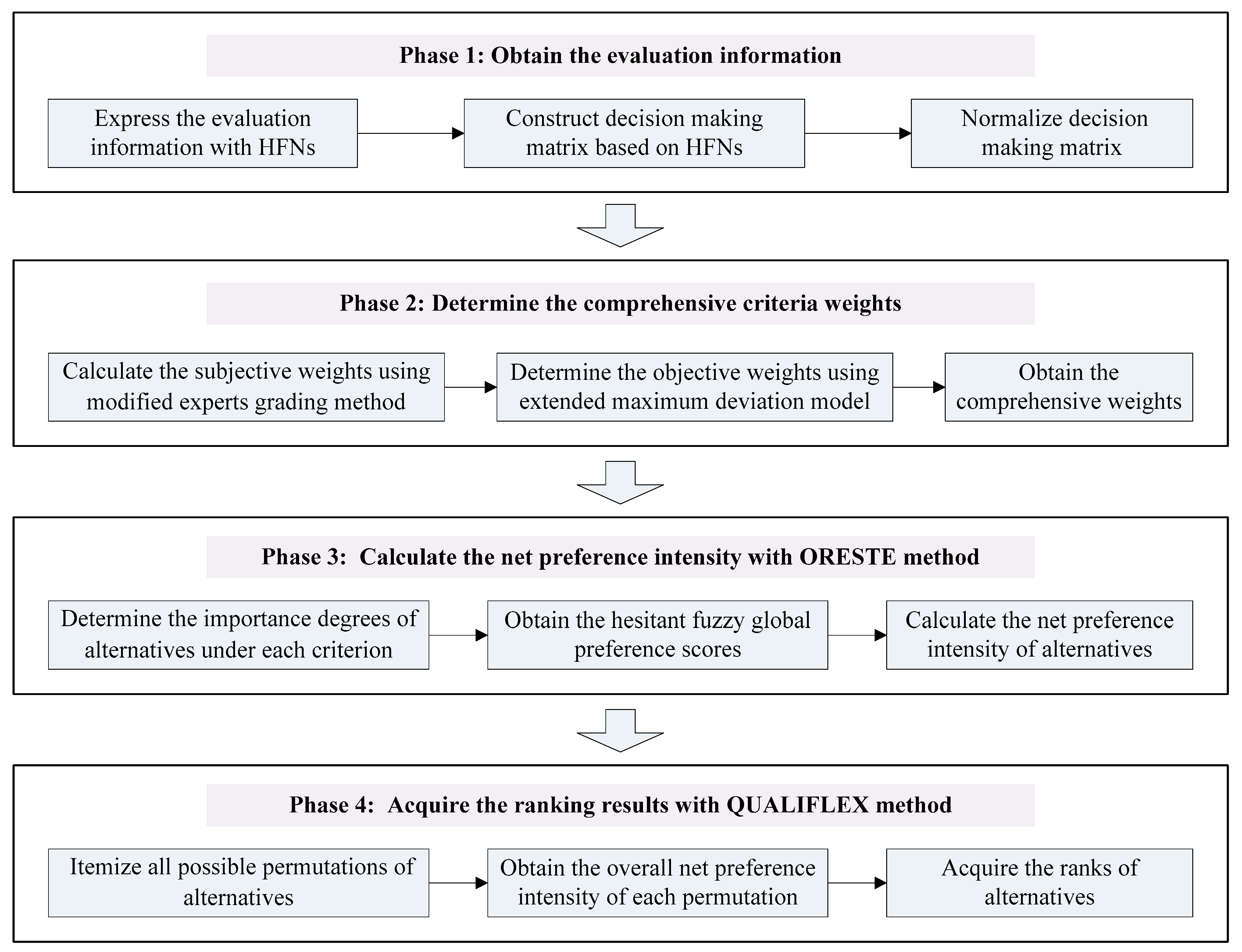
3.2. Hesitant Fuzzy ORESTE–QUALIFLEX Method

A hesitant fuzzy ORESTE–QUALIFLEX method is presented and its framework depicted in Figure 1. This methodology integrates HFSs, combination weighting technique, ORESTE method, and QUALIFLEX approach simultaneously. Four phases are contained. First, the HFSs are recommended to express the assessment data, and the initial decision-making matrix is then normalized. Second, the expert grading approach and entropy weight model are combined to compute the comprehensive criteria importance degrees. Third, the ORESTE model extended with HFSs is adopted to calculate the net preference intensity. Fourth, the QUALIFLEX approach is employed to acquire the rank results. The detailed steps of the hesitant fuzzy ORESTE–QUALIFLEX method are displayed in Figure 1.

(1) Phase 1: Obtain the evaluation information

With regard to assessment problems in a group, the initial assessment values are often given by different participators. Suppose $g$ DMs $\left\{S_1,S_2,\cdots ,S_g\right\}$ are invited to make evaluation of $m$ alternatives $\left\{A_1,A_2,\cdots ,A_m\right\}$ with $n$ criteria $\left\{B_1,B_2,\cdots ,B_n\right\}$, the specific steps for obtaining the evaluation information are as follows.

Step 1: Express the assessment values with HFNs.

According to the materials provided by mines, DMs can express their preferences in the form of non-negative real numbers (no more than 1). A value closer to 1 implicates that the criterion of this alternative has a higher score. Then, their evaluation results can be transferred into HFNs. For instance, assume four DMs make assessments, the grades of $B_j$ for alternatives $A_i$ are 0.6, 0.8, 0.7, and 0.7; these assessment values can be expressed as a HFN $x_{ij}=\left\{0.6,0.8,0.7,0.7\right\}$. Compared with the average value of 0.7, the HFN can indicate original information more comprehensively and reliably.

Step 2: Construct decision-making matrix based on HFNs.

Using this information processing approach, the general assessment matrix is denoted as

$$X=\left[\begin{array}{cccc}{x}_{11}& x_{12}& \cdots & x_{1n}\\ x_{21}& x_{22}& \cdots & x_{2n}\\ ⋮& ⋮& \ddots & ⋮\\ x_{m1}& x_{m2}& \cdots & x_{mn}\end{array}\right]$$

(10)

where $x_{ij}=\{x_{ij}^1,x_{ij}^2,\cdots ,x_{ij}^g\}$ is a HFN, and $x_{ij}^g$ indicates the value of $A_i$ ($i=1,2,\cdots ,m$) for $B_j$ ($j=1,2,\cdots ,n$) provided by the $g\mathrm{th}$ decision-maker.

Step 3: Normalize decision-making matrix.

In consideration of the cost criteria, transformations should be conducted by Equation (6). Then, the normalized evaluation matrix is

$$X^N=\left[\begin{array}{cccc}{x}_{11}^N& x_{12}^N& \cdots & x_{1n}^N\\ x_{21}^N& x_{22}^N& \cdots & x_{2n}^N\\ ⋮& ⋮& \ddots & ⋮\\ x_{m1}^N& x_{m2}^N& \cdots & x_{mn}^N\end{array}\right].$$

(11)

(2) Phase 2: Calculate the comprehensive criteria weight values

Step 1: Compute the subjective weights with modified expert grading approach.

The subjective weights are determined by a modified expert grading approach. First, some specialists are invited to judge the significance of criteria with decimals between 0 and 1. A value closer to 1 represents a more significant criterion. Thereafter, the grades of criteria are transformed to HFNs. Accordingly, the grading results are acquired as

$$E=\left[\begin{array}{cccc}{e}_1& e_2& \cdots & e_n\end{array}\right]$$

(12)

where $e_j=\left\{e_j^1,e_j^2,\cdots ,e_j^q\right\}$, and $e_j^u$ demonstrates the score of criterion $B_j$ from the $q\mathrm{th}$ expert.

Based on Equation (8), the subjective weights can be determined by

$$w_j^S=\frac{F(e_j)}{{\displaystyle \sum _j^{n}F(e_j)}}.$$

(13)

Step 2: Determine the objective weights with extended maximum deviation technique.

The objective weights are determined by an extended maximum deviation model. When the assessment information among alternatives under a criterion has a significant variance, then this criterion is important for the ranking results and can be allocated a big weight [53]. The procedures of hesitant fuzzy maximum deviation technique are demonstrated below.

First, the score function of each criterion value is obtained based on Equation (8). and can be normalized by

$$y_{ij}=\frac{F(x_{ij}^N)}{{\displaystyle \sum _i^{m}F(x_{ij}^N)}}.$$

(14)

Then, the deviation degree of a certain alternative is determined by

$$C_{ij}(w_j)={\displaystyle \sum _{r=1}^m\left|y_{ij}-y_{rj}\right|w_j}.$$

(15)

The total deviation degrees are donated as

$$C(w)={\displaystyle \sum _{j=1}^n{\displaystyle \sum _{i=1}^m{C}_{ij}(w_j)}}={\displaystyle \sum _{j=1}^n{\displaystyle \sum _{i=1}^m{\displaystyle \sum _{r=1}^m\left|y_{ij}-y_{rj}\right|w_j}}}.$$

(16)

Consequently, the programming model is created as

$$\{\begin{array}{l}\max C(w)={\displaystyle \sum _{j=1}^n{\displaystyle \sum _{i=1}^m{\displaystyle \sum _{r=1}^m\left|y_{ij}-y_{rj}\right|w_j}}}\\ s.t{\displaystyle \sum _{j=1}^n{w}_j^2}=1,0\le w_j\le 1,j=1,2,\cdots ,n\end{array}.$$

(17)

To acquire the result, the Lagrange function is established as

$$L(w,\lambda )={\displaystyle \sum _{j=1}^n{\displaystyle \sum _{i=1}^m{\displaystyle \sum _{r=1}^m\left|y_{ij}-y_{rj}\right|w_j}}}+\frac{1}{2}\lambda ({\displaystyle \sum _{j=1}^n{w}_j^2}-1).$$

(18)

The partial deviation of this Lagrange function is

$$\{\begin{array}{l}\frac{\partial L(w,\lambda )}{\partial w}={\displaystyle \sum _{j=1}^n{\displaystyle \sum _{i=1}^m{\displaystyle \sum _{r=1}^m\left|y_{ij}-y_{rj}\right|+}}}\lambda {\displaystyle \sum _{j=1}^n{w}_j}=0\\ \frac{\partial L(w,\lambda )}{\partial \lambda }=\frac{1}{2}({\displaystyle \sum _{j=1}^n{w}_j^2}-1)=0\end{array}.$$

(19)

Therefore, the optimal result related to weight is

$$w_j^{\ast }=\frac{{\displaystyle \sum _{i=1}^m{\displaystyle \sum _{r=1}^m\left|y_{ij}-y_{rj}\right|}}}{\sqrt{{\displaystyle \sum _{j=1}^n[{\displaystyle \sum _{i=1}^m{\displaystyle \sum _{r=1}^m\left|y_{ij}-y_{rj}\right|{]}^2}}}}}.$$

(20)

Finally, the objective weights can be obtained by

$$w_j^O=\frac{w_j^{\ast }}{{\displaystyle \sum _{j=1}^n{w}_j^{\ast }}}.$$

(21)

Step 3: Obtain the comprehensive weight values.

By combining the subjective and objective criteria weights, the comprehensive weight values are

$$w_j=\beta ·w_j^S+(1-\beta )·w_j^O$$

(22)

where $\beta \in [0,1]$ is a preference coefficient.

(3) Phase 3: Calculate the net preference intensity with ORESTE method

The ORESTE is used to compute the net preference intensity, and the specific steps are indicated below.

Step 1: Determine the importance degrees of alternatives under each criterion.

Borrowing the idea of TOPSIS, the importance degree $D_{ij}$ of alternative $A_i$ under criterion $B_j$ is

$$D_{ij}=\frac{d(x_{ij}^N\ge x_j^{-})}{d(x_{ij}^N\ge x_j^{+})+d(x_{ij}^N\ge x_j^{-})}$$

(23)

where $x_j^{+}=\underset{i}{\max }\left\{x_{ij}^N\right\}(j=1,2,\dots ,n)$ is the positive ideal value, $x_j^{-}=\underset{i}{\min }\left\{x_{ij}^N\right\}(j=1,2,\dots ,n)$ is the negative ideal value, $d(x_{ij}^N\ge x_j^{+})$ and $d(x_{ij}^N\ge x_j^{-})$ are the distance degrees calculated with Equation (7).

Step 2: Obtain the hesitant fuzzy global preference scores.

Suppose $\delta \in [0,1]$ is a balance number to implicate the relative importance of $w_j$ and $D_{ij}$, then the hesitant fuzzy global preference score $E_{ij}$ can be calculated with

$$E_{ij}=\sqrt{\delta {(w_j)}^2+(1-\delta ){(D_{ij})}^2}.$$

(24)

Step 3: Calculate the net preference intensity of alternatives.

The net preference intensity $∆G_{ik}$ can be obtained with

$$∆G_{ik}=G(A_i,A_k)-G(A_k,A_i)$$

(25)

where $G(A_i,A_k)=\frac{{\displaystyle {\sum }_{j=1}^n\max \{(E_{ij}-E_{kj}),0\}}}{n}$ is the average preference intensity of $A_i$ $(i=1,2,\cdots ,m)$ to $A_k$ $(k=1,2,\cdots ,m)$.

(4) Phase 4: Acquire the ranking results with QUALIFLEX method

The QUALIFLEX method based on the net preference intensity is utilized to rank alternatives. The concrete procedures are displayed below.

Step 1: Itemize all possible permutations of alternatives.

Because there are $m$ alternatives, $m!$ possible permutations can be found, and each permutation is denoted as

$$P_u=(\cdots ,A_i,\cdots ,A_k,\cdots )(u=1,2,\cdots ,m!)$$

(26)

where $A_i$ is the alternative that is no less than $A_k$.

Step 2: Obtain the overall net preference intensity of each permutation.

The overall net preference intensity of each permutation can be obtained with

$${∆}_u={\displaystyle \sum _{i=1}^{m-1}{\displaystyle \sum _{k=i+1}^m∆G_{ik}}}(u=1,2,\cdots ,m!).$$

(27)

Step 3: Acquire the ranks of alternatives.

According to the values of ${∆}_u$ ($u=1,2,\cdots ,m!$), the best permutation can be determined. That is to say, a bigger ${∆}_u$ value means a better permutation $P_u$. Then, the ranks of alternatives can also be acquired.

4. Case Study

The presented hesitant fuzzy ORESTE–QUALIFLEX methodology is employed to evaluate the performance of green mines in this section.

4.1. Engineering Background Description

Considering that current mining activities often cause some serious problems, such as environmental destruction, loss of resources, and safety incidents, the construction of green mines has become one of the most important measures in China. In 2007, the Ministry of Land and Resources of the People’s Republic of China (MLRPRC) first proposed the initiative of green mining in China. In 2009, the China Mining Association issued the convention of green mining. In 2010, the MLRPRC promulgated the basic conditions of green mines. In 2011 and 2012, the MLRPRC announced 220 pilot units of green mines twice successively. Until 2017, 661 mines have become pilot units of green mines. In 2018, the Ministry of Natural Resources of the People’s Republic of China released the industry standard for green mine construction. The concept of green mines has been extensively spread and constantly developed in China.

To achieve sustainable development, a large phosphorus chemical company in China has expended major efforts for the construction of green mines. Recently, this company announced it intended to apply for one of its mines to become a green mine. After comprehensive analysis and screening, four phosphorus mines (denoted as $A_1$, $A_2$, $A_3$, and $A_4$) did well in the construction of green mines and met the requirements of the application. For the sake of increasing the success rate of the application, it is essential to select the optimal one based on their comprehensive performance.

4.2. Assessment Criteria System of Green Mines

Selecting suitable criteria is essential for the performance evaluation of green mines. Some documents on the requirements of green mines have been issued by the government, which can effectively guide the construction of green mines. Based on the industry standards for green mine construction [54], the evaluation criteria system was established from six aspects: mining area environment ($B_1$), resource development approaches ($B_2$), comprehensive utilization of resources ($B_3$), energy conservation and emission reduction ($B_4$), technological innovation ($B_5$), and management level ($B_6$). The detailed descriptions of these criteria are demonstrated in

Table 2. Evaluation criteria of green mines.

Evaluation Criteria	Descriptions
Mining area environment $B_1$	This refers to the environment of the mining area and mainly includes appearance of the mining area, layout of function, and greening of the mining area.
Resource development approaches $B_2$	This refers to the superiority of development approaches and mainly includes mining technology, environmental monitoring, and environmental restoration.
Comprehensive utilization of resources $B_3$	This refers to the comprehensive utilization of resources and mainly includes the utilization of solid waste, wastewater, and associated resources.
Energy conservation and emission reduction $B_4$	This refers to the saving of energy and emission of various pollutants and mainly includes energy conservation, discharge of solid waste, wastewater, exhaust gas, and dust.
Technological innovation $B_5$	This refers to the level of technical innovation and mainly includes innovation ability, automation performance, and digital mine.
Management level $B_6$	This refers to the management level of enterprise and mainly includes the culture, management, and credit of enterprise, social stability, and responsibility.

.

4.3. Performance Assessment of Green Mines

In Phase 1, to assess the performance of these four mines fairly, four experts (denoted as $S_1$, $S_2$, $S_3$, and $S_4$) familiar with this field were invited to make evaluations anonymously according to the submitted application materials. They gave their evaluation results with no more than 1 decimal place. Then, their assessment results were merged and converted into HFNs. The original assessment matrix is indicated in

Table 3. Initial assessment matrix $X$.

	${\mathit{B}}_1$	${\mathit{B}}_2$	${\mathit{B}}_3$	${\mathit{B}}_4$	${\mathit{B}}_5$	${\mathit{B}}_6$
$A_1$	{0.5,0.7,0.6,0.6}	{0.8,0.7,0.7,0.7}	{0.9,0.8,0.9,0.7}	{0.7,0.6,0.6,0.7}	{0.6,0.7,0.6,0.5}	{0.6,0.5,0.5,0.7}
$A_2$	{0.9,0.7,0.9,0.8}	{0.7,0.7,0.6,0.6}	{0.6,0.7,0.8,0.6}	{0.7,0.6,0.5,0.5}	{0.5,0.6,0.6,0.5}	{0.7,0.8,0.8,0.7}
$A_3$	{0.7,0.8,0.7,0.8}	{0.9,0.7,0.8,0.7}	{0.6,0.8,0.8,0.7}	{0.9,0.8,0.9,0.7}	{0.8,0.7,0.6,0.7}	{0.8,0.8,0.7,0.8}
$A_4$	{0.7,0.6,0.6,0.5}	{0.7,0.5,0.6,0.6}	{0.5,0.6,0.5,0.7}	{0.8,0.7,0.8,0.9}	{0.7,0.9,0.7,0.7}	{0.6,0.7,0.7,0.8}

. As all evaluation criteria belonged to benefit type, the normalized assessment matrix $X^N$ was equal to $X$.

In Phase 2, the subjective weight values were determined using the hesitant fuzzy expert grading approach. The above four experts gave evaluations about criteria with decimals. The assessment results are displayed in

Table 4. Importance degrees of criteria.

	${\mathit{B}}_1$	${\mathit{B}}_2$	${\mathit{B}}_3$	${\mathit{B}}_4$	${\mathit{B}}_5$	${\mathit{B}}_6$
$S_1$	0.6	0.8	0.8	0.7	0.8	0.7
$S_2$	0.8	0.7	0.7	0.8	0.9	0.8
$S_3$	0.7	0.8	0.9	0.7	0.9	0.8
$S_4$	0.8	0.8	0.8	0.8	0.8	0.9
$e_j$	{0.6,0.8,0.7,0.8}	{0.8,0.7,0.8,0.8}	{0.8,0.7,0.9,0.8}	{0.7,0.8,0.7,0.8}	{0.8,0.9,0.9,0.8}	{0.7,0.8,0.8,0.9}
$F(e_j)$	0.7200	0.7737	0.7969	0.7483	0.8485	0.7969
$w_j^S$	0.1537	0.1652	0.1701	0.1597	0.1811	0.1701

. Then, their scores of criteria were transformed into HFNs (see the fifth row in Table 4). Based on Equation (8), the score function $F\left(e_j\right)$ of each HFN was obtained (see the sixth row in Table 4). Lastly, the subjective weight $w_j^S$ was calculated using Equation (13) (see the last row in Table 4).

The objective criteria weights were obtained using the extended maximum deviation model. First, the normalized score function values were determined according to Equations (8) and (14) (see

Table 5. Normalized score function values $y_{ij}$.

	${\mathit{B}}_1$	${\mathit{B}}_2$	${\mathit{B}}_3$	${\mathit{B}}_4$	${\mathit{B}}_5$	${\mathit{B}}_6$
A1	0.2158	0.2643	0.2952	0.2286	0.2305	0.2042
A2	0.2973	0.2367	0.2410	0.2008	0.2119	0.2684
A3	0.2711	0.2814	0.2590	0.2895	0.2694	0.2776
A4	0.2158	0.2176	0.2047	0.2811	0.2883	0.2498

). Then, based on Equations (15)–(20), the optimal solution of weight was calculated as follows: $w_1^{\ast }=0.5993$, $w_2^{\ast }=0.4385$, $w_3^{\ast }=0.5787$, $w_4^{\ast }=0.6373$, $w_5^{\ast }=0.5366$, and $w_6^{\ast }=0.4774$. Therefore, the objective weights were obtained using Equation (21) as follows: $w_1^O=0.1834$, $w_2^O=0.1342$, $w_3^O=0.1771$, $w_4^O=0.1950$, $w_5^O=0.1642$, and $w_6^O=0.1461$.

Finally, supposing $\beta =0.5$, the comprehensive weights were determined using Equation (22). as follows: $w_1=0.1685$, $w_2=0.1497$, $w_3=0.1736$, $w_4=0.1774$, $w_5=0.1727$, and $w_6=0.1581$.

In Phase 3, based on Equation (9), the positive ideal solution was obtained as follows: $x_1^{+}=x_{21}^N=\{0.9,0.7,0.9,0.8\}$, $x_2^{+}=x_{32}^N=\{0.9,0.7,0.8,0.7\}$, $x_3^{+}=x_{13}^N=\{0.9,0.8,0.9,0.7\}$, $x_4^{+}=x_{34}^N=\{0.9,0.8,0.9,0.7\}$, $x_5^{+}=x_{45}^N=\{0.7,0.9,0.7,0.7\}$ and $x_6^{+}=x_{36}^N=\{0.8,0.8,0.7,0.8\}$. The negative ideal solution was as follows: $x_1^{-}=x_{11}^N=\{0.5,0.7,0.6,0.6\}$, $x_2^{-}=x_{42}^N=\{0.7,0.5,0.6,0.6\}$, $x_3^{-}=x_{43}^N=\{0.5,0.6,0.5,0.7\}$, $x_4^{-}=x_{24}^N=\{0.7,0.6,0.5,0.5\}$, $x_5^{-}=x_{25}^N=\{0.5,0.6,0.6,0.5\}$, and $x_6^{-}=x_{16}^N=\{0.6,0.5,0.5,0.7\}$. After that, according to Equation (23), the importance degrees of alternatives under each criterion were calculated, as shown in

Table 6. Importance degree $D_{ij}$.

${\mathit{D}}_{\mathit{i}\mathit{j}}$	${\mathit{B}}_1$	${\mathit{B}}_2$	${\mathit{B}}_3$	${\mathit{B}}_4$	${\mathit{B}}_5$	${\mathit{B}}_6$
$A_1$	0.0000	0.6517	1.0000	0.3245	0.3090	0.0000
$A_2$	1.0000	0.3483	0.3874	0.0000	0.0000	0.7829
$A_3$	0.6461	1.0000	0.6126	1.0000	0.6910	1.0000
$A_4$	0.0000	0.0000	0.0000	0.8209	1.0000	0.6044

.

Letting $\delta =0.5$, on the basis of Equation (24), the hesitant fuzzy global preference score $E_{ij}$ was calculated, as shown in

Table 7. Hesitant fuzzy global preference score $E_{ij}$.

${\mathit{E}}_{\mathit{i}\mathit{j}}$	${\mathit{B}}_1$	${\mathit{B}}_2$	${\mathit{B}}_3$	${\mathit{B}}_4$	${\mathit{B}}_5$	${\mathit{B}}_6$
$A_1$	0.1192	0.4728	0.7177	0.2615	0.2503	0.1118
$A_2$	0.7171	0.2681	0.3002	0.1254	0.1221	0.5647
$A_3$	0.4722	0.7150	0.4502	0.7181	0.5036	0.7159
$A_4$	0.1192	0.1058	0.1228	0.5938	0.7176	0.4417

.

Thereafter, based on Equation (25), the net preference intensity ∆G_ik of each alternative was obtained, as shown in

Table 8. Net preference intensity $∆G_{ik}$.

$∆G_{ik}$	${\mathit{A}}_1$	${\mathit{A}}_2$	${\mathit{A}}_3$	${\mathit{A}}_4$
A1	0.0000	−0.0274	−0.2736	−0.0279
$A_2$	0.0274	0.0000	−0.2462	−0.0005
$A_3$	0.2736	0.2462	0.0000	0.2457
$A_4$	0.0279	0.0005	−0.2457	0.0000

.

In Phase 4, there were 24 possible permutations: $P_1=(A_1,A_2,A_3,A_4)$, $P_2=(A_1,A_2,A_4,A_3)$, $P_3=(A_1,A_3,A_2,A_4)$, $P_4=(A_1,A_3,A_4,A_2)$, $P_5=(A_1,A_4,A_2,A_3)$, $P_6=(A_1,A_4,A_3,A_2)$, $P_7=(A_2,A_1,A_3,A_4)$, $P_8=(A_2,A_1,A_4,A_3)$, $P_9=(A_2,A_3,A_1,A_4)$, $P_{10}=(A_2,A_3,A_4,A_1)$, $P_{11}=(A_2,A_4,A_1,A_3)$, $P_{12}=(A_2,A_4,A_3,A_1)$, $P_{13}=(A_3,A_1,A_2,A_4)$, $P_{14}=(A_3,A_1,A_4,A_2)$, $P_{15}=(A_3,A_2,A_1,A_4)$, $P_{16}=(A_3,A_2,A_4,A_1)$, $P_{17}=(A_3,A_4,A_1,A_2)$, $P_{18}=(A_3,A_4,A_2,A_1)$, $P_{19}=(A_4,A_1,A_2,A_3)$, $P_{20}=(A_4,A_1,A_3,A_2)$, $P_{21}=(A_4,A_2,A_1,A_3)$, $P_{22}=(A_4,A_2,A_3,A_1)$, $P_{23}=(A_4,A_3,A_1,A_2)$, and $P_{24}=(A_4,A_3,A_2,A_1)$. On the basis of Equation (27), the overall net preference intensity ${∆}_u$ of each permutation was computed, as shown in

Table 9. Overall net preference intensity ${∆}_u$.

${∆}_1$	${∆}_2$	${∆}_3$	${∆}_4$	${∆}_5$	${∆}_6$	${∆}_7$	${∆}_8$
−0.3301	−0.8214	0.1624	0.1635	−0.8203	−0.3279	−0.2753	−0.7666
${∆}_9$	∆10	${∆}_{11}$	${∆}_{12}$	${∆}_{13}$	${∆}_{14}$	${∆}_{15}$	${∆}_{16}$
0.2720	0.3279	−0.7108	−0.1635	0.7097	0.7381	0.7644	0.8203
${∆}_{17}$	${∆}_{18}$	${∆}_{19}$	${∆}_{20}$	${∆}_{21}$	${∆}_{22}$	${∆}_{23}$	∆24
0.7666	0.8214	−0.7644	−0.2720	−0.7097	−0.1624	0.2753	0.3301

.

Because the value of ${∆}_{18}=0.8214$ was the biggest, the best rank was $P_{18}=(A_3,A_4,A_2,A_1)$. In other words, $A_3\succ A_4\succ A_2\succ A_1$, and the optimal phosphorus mine was $A_3$.

5. Discussions

In this section, sensitivity and comparison analyses are adopted to show the robustness, efficiency, and strengths of the proposed method.

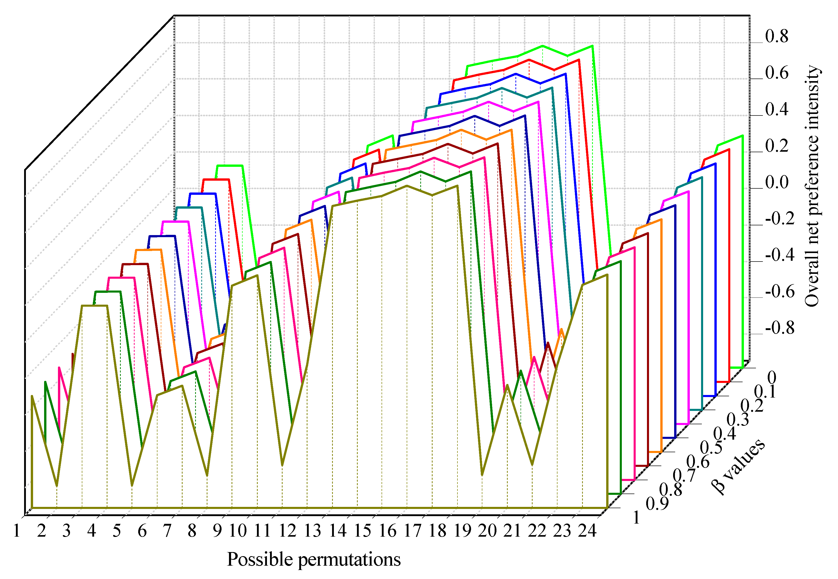
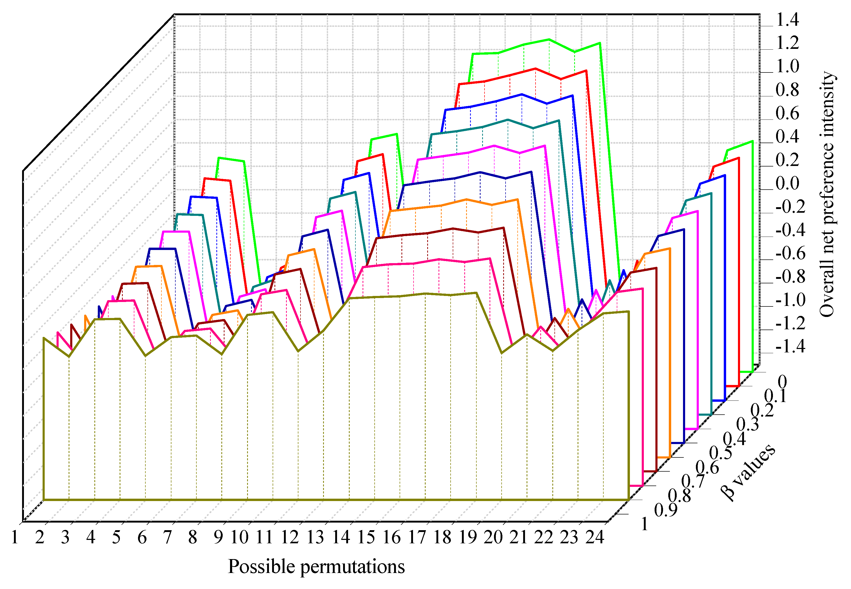
5.1. Sensitivity Analysis

The preference coefficient $\beta$ in Equation (22) was introduced to adjust the proportion of subjective and objective weights. In the case study of this research, the preference of subjective weight and objective weight was regarded as identical, i.e., $\beta =0.5$. However, the value of $\beta$ may be diverse for different DMs. When DMs highlight the subjective weight, a large $\beta$ value will be given, i.e., $0.5<\beta \le 1$. By contrast, a small $\beta$ value is assigned when experts highlight the objective weight, i.e., $0\le \beta <0.5$. The $\beta$ value directly affects the comprehensive weights and may have an important influence on the final evaluation results. Therefore, it is essential to investigate the impacts of different $\beta$ values on the ranking results.

To verify the specific effect on the evaluation results, other β values, such as 0, 0.1, 0.2, 0.3, 0.4, 0.6, 0.7, 0.8, 0.9, and 1 were chosen as comparisons. The overall net preference intensity ${∆}_u$ of various $\beta$ values for each permutation is displayed in Figure 2. It can be seen that the trends of ${∆}_u$ for each permutation were similar when different $\beta$ values were provided. For clarity, the results with diverse values of $\beta$ are indicated in

Table 10. Ranking results with different $\beta$ values ($\delta =0.5$).

$\mathit{\beta }$	Rank	$\mathit{\beta }$	Rank
0	$A_3\succ A_4\succ A_2\succ A_1$	0.6	$A_3\succ A_4\succ A_2\succ A_1$
0.1	$A_3\succ A_4\succ A_2\succ A_1$	0.7	$A_3\succ A_4\succ A_2\succ A_1$
0.2	$A_3\succ A_4\succ A_2\succ A_1$	0.8	$A_3\succ A_4\succ A_2\succ A_1$
0.3	$A_3\succ A_4\succ A_2\succ A_1$	0.9	$A_3\succ A_4\succ A_2\succ A_1$
0.4	$A_3\succ A_4\succ A_2\succ A_1$	1	$A_3\succ A_4\succ A_2\succ A_1$
0.5	$A_3\succ A_4\succ A_2\succ A_1$

. Obviously, the ranking results were always $A_3\succ A_4\succ A_2\succ A_1$. In other words, the ranking was insensitive to the parameter $\beta$, which verifies the robustness of the methodology.

In addition, the parameter $\delta$ in Equation (24) had some effects on the final evaluation results. In this research, the value of $\delta$ was assigned as 0.5. However, other $\delta$ values may be chosen by different DMs. Accordingly, some $\delta$ values, such as 0, 0.1, 0.2, 0.3, 0.4, 0.6, 0.7, 0.8, 0.9, and 1, were selected as contrasts to analyze the concrete influence. The overall net preference intensity ${∆}_u$ of various $\delta$ values is demonstrated in Figure 3. According to the value of ${∆}_u$, the optimal permutation was determined, and the results with dissimilar values of $\delta$ are shown in

Table 11. Ranking orders with different $\delta$ values ($\beta =0.5$).

$\mathit{\delta }$	Rank	$\mathit{\delta }$	Rank
0	$A_3\succ A_2\succ A_4\succ A_1$	0.6	$A_3\succ A_4\succ A_2\succ A_1$
0.1	$A_3\succ A_2\succ A_4\succ A_1$	0.7	$A_3\succ A_4\succ A_2\succ A_1$
0.2	$A_3\succ A_2\succ A_4\succ A_1$	0.8	$A_3\succ A_4\succ A_2\succ A_1$
0.3	$A_3\succ A_2\succ A_4\succ A_1$	0.9	$A_3\succ A_4\succ A_2\succ A_1$
0.4	$A_3\succ A_2\succ A_4\succ A_1$	1	--
0.5	$A_3\succ A_4\succ A_2\succ A_1$

. It is clear that, when $\delta$ values were 0, 0.1, 0.2, 0.3, and 0.4, the ranking results were $A_3\succ A_2\succ A_4\succ A_1$, respectively; when $\delta$ values were 0.5, 0.6, 0.7, 0.8, and 0.9, the ranking results were $A_3\succ A_4\succ A_2\succ A_1$, respectively; and when $\delta$ value was 1, the ranking result was inactive. Consequently, the $\delta$ values directly affected the evaluation results. However, the optimal and worst alternatives were always $A_3$ and A₁, respectively. As the aim of this case was to choose the best option, the evaluation results of adopting our approach was relatively stable.

5.2. Comparison Analysis

Several existing MCDM methods based on HFSs, such as the TOPSIS [19], TODIM [22], VIKOR [21], and QUALIFLEX method [26], were used as comparisons with the proposed methodology.

Firstly, the TOPSIS method based on HFSs was recommended to acquire the evaluation result. The Euclidean distances from the positive ideal values were $d_1^{+}=0.1420$, $d_2^{+}=0.1370$, $d_3^{+}=0.0442$, and $d_4^{+}=0.1324$. The Euclidean distances from the negative ideal values were $d_1^{-}=0.0916$, $d_2^{-}=0.0951$, $d_3^{-}=0.1872$, and $d_4^{-}=0.0982$. The relative closeness was ${\theta }_1=0.3922$, ${\theta }_2=0.4096$, ${\theta }_3=0.8091$, and ${\theta }_4=0.4258$. Because ${\theta }_3>{\theta }_4>{\theta }_2>{\theta }_1$, the ranking result was $A_3\succ A_4\succ A_2\succ A_1$.

Secondly, the TODIM method based on HFSs was used to determine the evaluation result. The dominance of each alternative over other alternatives was $\delta (A_i,A_k)=\left[\begin{array}{rrrr}\hfill 0.0000& \hfill -0.7626& \hfill -2.5323& \hfill -0.5930\\ \hfill -2.2172& \hfill 0.0000& \hfill -2.6563& \hfill -0.7054\\ \hfill -0.3140& \hfill -0.2527& \hfill 0.0000& \hfill 0.5874\\ \hfill -1.9844& \hfill -2.4107& \hfill -3.5513& \hfill 0.0000\end{array}\right]$. Then, the global values of alternatives were ${\pi }_1=0.5094$, ${\pi }_2=0.2972$, ${\pi }_3=1$, and ${\pi }_4=0$. Because ${\pi }_3>{\pi }_1>{\pi }_2>{\pi }_4$, the ranking result was $A_3\succ A_1\succ A_2\succ A_4$.

Thirdly, the VIKOR approach with HFSs was employed to determine the evaluation result. The group benefit values were $G_1=0.6395$, $G_2=0.6049$, $G_3=0.1893$, and $G_4=0.5911$. The individual regret values were $I_1=0.1685$, $I_2=0.1774$, $I_3=0.0681$, and $I_4=0.1736$. Supposing the proportion for the scheme of maximum group utility was 0.5, the compromise sorting index values were $Z_1=0.9593$, $Z_2=0.9616$, $Z_3=0$, and $Z_4=0.9289$. As $Z_3<Z_4<Z_1<Z_2$, the ranking result was $A_3\succ A_4\succ A_1\succ A_2$.

Fourthly, the QUALIFLEX approach with HFSs was introduced to determine the evaluation result. The score function defined in Equation (8). was utilized to calculate the concordance index, and the overall concordance index of each permutation is listed in

Table 12. Overall concordance index ${\Theta }_u$.

${\Theta }_1$	${\Theta }_2$	${\Theta }_3$	${\Theta }_4$	${\Theta }_5$	${\Theta }_6$	${\Theta }_7$	${\Theta }_8$
−0.1281	−0.2959	0.0521	0.0646	−0.2834	−0.1032	−0.1153	−0.2830
${\Theta }_9$	${\Theta }_{10}$	${\Theta }_{11}$	Θ12	${\Theta }_{13}$	${\Theta }_{14}$	${\Theta }_{15}$	${\Theta }_{16}$
0.0778	0.1032	−0.2577	−0.0646	0.2452	0.2641	0.2581	0.2834
${\Theta }_{17}$	${\Theta }_{18}$	${\Theta }_{19}$	${\Theta }_{20}$	${\Theta }_{21}$	Θ22	${\Theta }_{23}$	${\Theta }_{24}$
0.2830	0.2959	−0.2581	−0.0778	−0.2452	−0.0521	0.1153	0.1281

. As the value of ${\Theta }_{18}=0.2959$ was the biggest, the best rank would be $P_{18}=(A_3,A_4,A_2,A_1)$, namely, $A_3\succ A_4\succ A_2\succ A_1$.

To further demonstrate the advantages of our method, the traditional ORESTE was integrated with HFSs to determine the evaluation result. Supposing the preference threshold value was 0.01 and the incomparability threshold value was 0.005, then the PIR structure of alternatives is shown in

Table 13. Preference, indifference, and incomparability (PIR) structure of alternatives.

	${\mathit{A}}_1$	${\mathit{A}}_2$	${\mathit{A}}_3$	${\mathit{A}}_4$
$A_1$	-	R	R	R
$A_2$	P	-	R	I
$A_3$	P	P	-	P
A4	P	I	R	-

. According to Table 13, the strong rank order of $A_3\succ \{A_2,A_4\}\succ A_1$ was obtained.

Finally, the results of dissimilar methods are shown in

Table 14. Evaluation results with dissimilar approaches.

Approach	Rank	The Best Alternative	The Worst Alternative
TOPSIS [19]	$A_3\succ A_4\succ A_2\succ A_1$	$A_3$	$A_1$
TODIM [22]	$A_3\succ A_1\succ A_2\succ A_4$	$A_3$	$A_4$
VIKOR [21]	$A_3\succ A_4\succ A_1\succ A_2$	$A_3$	$A_2$
QUALIFLEX [26]	$A_3\succ A_4\succ A_2\succ A_1$	$A_3$	$A_1$
ORESTE	$A_3\succ \{A_2,A_4\}\succ A_1$	$A_3$	$A_1$
The proposed approach	$A_3\succ A_4\succ A_2\succ A_1$	$A_3$	$A_1$

.

From Table 14, dissimilar ranking orders were acquired when distinct approaches were applied. For determining the optimal ranking order, the dominance theory was adopted. That is to say, a better rank of an alternative in a certain ranking order was allocated with a larger score, and the optimal rank was attained based on the score of each alternative. Taking $A_3\succ A_4\succ A_2\succ A_1$ as an example, as $A_3$ ranked first, it was assigned with 4, $A_4$ (the second rank) was 3, $A_2$ (the third rank) was 2, and $A_1$ (the last rank) was 1. Likewise, the final score of each alternative was as follows: $S(A_1)=9$, $S(A_2)=11.5$, $S(A_3)=24$, and $S(A_4)=15.5$. Because $S(A_3)>S(A_4)>S(A_2)>S(A_1)$, then the optimal rank was $A_3\succ A_4\succ A_2\succ A_1$. It is clear that this ranking order was the same as that of TOPSIS, QUALIFLEX, and our method. Furthermore, the best option was always $A_3$ in Table 14, and the worst option was $A_1$ in most cases. These results can verify the feasibility of our method.

The same ranking orders were obtained with TOPSIS, QUALILFEX, and the proposed method. Compared with them, our method is more flexible with two adjustment parameters. Compared with QUALIFLEX, our method considers the preferences of both criteria weights and original information by combining ORESTE, while only the impacts of score function are considered in QUALIFLEX.

Compared with VIKOR, the proposed method can always obtain a complete rank. Even though a complete rank was also obtained with VIKOR in our example, it may be that just a compromise solution can be found in other cases. For instance, if the sequences of the group utility and individual regret are inconsistent or some requirements are not satisfied, then only a compromise solution can be acquired.

Compared with the traditional ORESTE, the proposed approach calculates the crisp weight values (instead of the Besson’s rank) of criteria to acquire more information. As shown, only a compromise solution $A_3\succ \{A_2,A_4\}\succ A_1$ was obtained with the ORESTE method in our example. That is to say, the preference relation of alternatives $A_2$ and $A_4$ was undetermined with ORESTE. Therefore, the ORESTE would be invalid when DMs plan to select a relatively better alternative between $A_2$ and $A_4$. The proposed method combined the ORESTE with QUALIFLEX to get a complete ranking order, i.e., $A_3\succ A_4\succ A_2\succ A_1$.

Accordingly, the highlights of our method are summarized as follows:

(1) HFSs are recommended to depict original assessment information with a set of possible membership function values. As a result, all the opinions (especially different opinions) of DMs in a group can be completely contained and expressed with HFSs.

(2) The subjective predilections of criteria are considered by extending the expert grading method under hesitant fuzzy conditions. At the same time, the objective facts are not ignored by modifying the maximum deviation model with HFSs.

(3) The traditional QUALIFLEX is integrated with the ORESTE method. On the one hand, more information can be obtained with the net preference intensity, and the parameter in ORESTE can enhance the flexibility of our approach. On the other hand, the idea of itemizing all possible permutations in QUALILFLEX is simple but effective, especially when many criteria exist. Furthermore, a complete rank of alternatives can be guaranteed with QUALIFLEX.

6. Conclusions

This research focused on assessing the performance of green mines using a hesitant fuzzy ORESTE–QUALIFLEX method. The motivation for the research came from the following aspects. First, the construction of green mines is essential for the sustainable development of mine enterprises, but little literature related to exclusively solving performance evaluation problems of green mines exists. Second, the decision-making values are real numbers in the existing literature, and some fuzzy evaluation information provided by experts cannot be expressed. Third, as we know, fuzzy decision-making methods have not been adopted so far to assess the performance of green mines. As the number of evaluation criteria is usually more than that of the evaluated mines, the QUALIFLEX method was first considered. In addition, the idea of ORESETE method was used to overcome the limitations of the traditional QUALIFLEX method.

In summary, the main contributions of this research are as follows: (1) The initial criteria weights were represented by HFSs so that the qualitative assessment information could be indicated more reliably and comprehensively. (2) A comprehensive weighting approach combining the extended expert grading approach and maximum deviation technique was proposed to calculate the criteria weight values. Thus, both subjective preferences and objective facts were considered under hesitant fuzzy circumstances. (3) The traditional QUALIFLEX approach was extended with ORESTE so that their advantages were utilized. The ORESTE method was used to determine the net preference intensity, and the QUALIFLEX was utilized to rank alternatives. The feasibility of our approach was illustrated by a case study evaluating the performance of green mines in China. (4) The sensitivity and comparison analyses indicated that the proposed methodology has great robustness and strengths. Therefore, the proposed hesitant fuzzy ORESTE–QUALIFLEX framework can be adopted to appraise the performance of green mines, and reliable and stable evaluation results can be acquired.

Future studies may be conducted in some potential directions. For example, the proposed hesitant fuzzy ORESTE–QUALIFLEX method can also be applied to solve similar evaluation problems under hesitant fuzzy environment in other fields, such as the performance evaluation of cleaner production. Furthermore, even though satisfactory results were obtained with our method, the combination of two models still makes it a little complex. Thus, simpler and more effective fuzzy MCDM approaches can be investigated to assess the performance of green mines.

References

1. Ali, S.H.; Giurco, D.; Arndt, N.; Nickless, E.; Brown, G.; Demetriades, A.; Durrheim, R.; Enriquez, M.A.; Kinnaird, J.; Littleboy, A.; et al. Mineral supply for sustainable development requires resource governance. Nature 2017, 543, 367–372. [Google Scholar] [CrossRef] [PubMed]
2. Luo, S.Z.; Liang, W.Z.; Xing, L.N. Selection of mine development scheme based on similarity measure under fuzzy environment. Neural Comput. Appl. 2019, 1–12. [Google Scholar] [CrossRef]
3. Sun, S.Y.; Sun, H.; Zhang, D.S.; Zhang, J.F.; Cai, Z.Y.; Qin, G.H.; Song, Y.M. Response of soil microbes to vegetation restoration in coal mining subsidence areas at Huaibei coal mine China. Int. J. Environ. Res. Public Health 2019, 16, 1757. [Google Scholar] [CrossRef] [PubMed]
4. Liang, W.Z.; Zhao, G.Y.; Wu, H.; Dai, B. Risk assessment of rockburst via an extended MABAC method under fuzzy environment. Tunn. Undergr. Space Tech. 2019, 83, 533–544. [Google Scholar] [CrossRef]
5. Timofeev, I.; Kosheleva, N.; Kasimov, N. Contamination of soils by potentially toxic elements in the impact zone of tungsten—Molybdenum ore mine in the Baikal region: A survey and risk assessment. Sci. Total. Environ. 2018, 642, 63–76. [Google Scholar] [CrossRef] [PubMed]
6. Shang, D.L.; Yin, G.Z.; Li, X.S.; Li, Y.J.; Jiang, C.B.; Kang, X.T.; Liu, C.; Zhang, C. Analysis for green mine (phosphate) performance of China: An evaluation index system. Resour. Policy 2015, 46, 71–84. [Google Scholar] [CrossRef]
7. Wang, W.S.; Zou, J.L. Efficiency evaluation and optimization of green mining construction in coal enterprises based on DEA. China Coal 2013, 39, 119–121. [Google Scholar]
8. Xu, J.Q.; Yu, G.; He, D.Y. Multi-expert evaluation method of Green Mine: A case study on Xinwen mining group’s Huafeng mine. Resour. Ind. 2016, 18, 61–68. [Google Scholar]
9. Hu, J.H.; Xiao, K.L.; Chen, X.H.; Liu, Y.M. Interval type-2 hesitant fuzzy set and its application in multi-criteria decision making. Comput. Ind. Eng. 2015, 87, 91–103. [Google Scholar] [CrossRef]
10. Luo, S.Z.; Zhang, H.Y.; Wang, J.Q.; Li, L. Group decision-making approach for evaluating the sustainability of constructed wetlands with probabilistic linguistic preference relations. J. Oper. Res. Soc. 2019, 1–17. [Google Scholar] [CrossRef]
11. Torra, V. Hesitant fuzzy sets. Int. J. Intell. Syst. 2010, 25, 529–539. [Google Scholar] [CrossRef]
12. Alcantud, J.C.R.; Torra, V. Decomposition theorems and extension principles for hesitant fuzzy sets. Inform. Fusion 2018, 41, 48–56. [Google Scholar] [CrossRef]
13. Torra, V.; Narukawa, Y. On hesitant fuzzy sets and decision. In Proceedings of the 18th IEEE International Conference on Fuzzy Systems, Jeju Island, Korea, 20–24 August 2009; pp. 1378–1382. [Google Scholar]
14. Rodríguez, R.M.; Martínez, L.; Torra, V.; Xu, Z.S.; Herrera, F. Hesitant fuzzy sets: state of the art and future directions. Int. J. Intell. Syst. 2014, 29, 495–524. [Google Scholar] [CrossRef]
15. Xu, Y.; Liu, L.Z.; Zhang, X.Y. Multilattices on typical hesitant fuzzy sets. Inform. Sci. 2019, 491, 63–73. [Google Scholar] [CrossRef]
16. Deveci, M.; Özcan, E.; John, R.; Öner, S.C. Interval type-2 hesitant fuzzy set method for improving the service quality of domestic airlines in Turkey. J. Air Trans. Manag. 2018, 69, 83–98. [Google Scholar] [CrossRef]
17. Iordache, M.; Schitea, D.; Deveci, M.; Akyurt, İ.Z.; Iordache, I. An integrated ARAS and interval type-2 hesitant fuzzy sets method for underground site selection: Seasonal hydrogen storage in salt caverns. J. Petrol. Sci. Eng. 2019, 175, 1088–1098. [Google Scholar] [CrossRef]
18. Iiang, W.Z.; Zhao, G.Y.; Wang, X.; Zhao, J.; Ma, C.D. Assessing the rockburst risk for deep shafts via distance-based multi-criteria decision making approaches with hesitant fuzzy information. Eng. Geol. 2019, 105211. [Google Scholar] [CrossRef]
19. Xu, Z.S.; Zhang, X.L. Hesitant fuzzy multi-attribute decision making based on TOPSIS with incomplete weight information. Knowl. Based Syst. 2013, 52, 53–64. [Google Scholar] [CrossRef]
20. Zeng, S.; Baležentis, A.; Su, W. The multi-criteria hesitant fuzzy group decision making with MULTIMOORA method. Econ. Comput. Econ. Cybern. 2013, 47, 171–184. [Google Scholar]
21. Zhang, N.; Wei, G.W. Extension of VIKOR method for decision making problem based on hesitant fuzzy set. Appl. Math. Model. 2013, 37, 4938–4947. [Google Scholar] [CrossRef]
22. Zhang, X.L.; Xu, Z.S. The TODIM analysis approach based on novel measured functions under hesitant fuzzy environment. Knowl. Based Syst. 2014, 61, 48–58. [Google Scholar] [CrossRef]
23. Zhang, X.L.; Xu, Z.S. Interval programming method for hesitant fuzzy multi-attribute group decision making with incomplete preference over alternatives. Comput. Ind. Eng. 2014, 75, 217–229. [Google Scholar] [CrossRef]
24. Chen, N.; Xu, Z.S.; Xia, M.M. The ELECTRE I multi-criteria decision-making method based on hesitant fuzzy sets. Int. J. Inf. Tech. Decis. 2015, 14, 621–657. [Google Scholar] [CrossRef]
25. Chen, N.; Xu, Z.S. Hesitant fuzzy ELECTRE II approach: A new way to handle multi-criteria decision making problems. Inform. Sci. 2015, 292, 175–197. [Google Scholar] [CrossRef]
26. Zhang, X.L.; Xu, Z.S. Hesitant fuzzy qualiflex approach with a signed distance-based comparison method for multiple criteria decision analysis. Expert Syst. Appl. 2015, 42, 873–884. [Google Scholar] [CrossRef]
27. Mahmoudi, A.; Sadi-Nezhad, S.; Makui, A.; Vakili, M.R. An extension on PROMETHEE based on the typical hesitant fuzzy sets to solve multi-attribute decision-making problem. Kybernetes 2016, 45, 1213–1231. [Google Scholar] [CrossRef]
28. Acar, C.; Beskese, A.; Temur, G.T. Sustainability analysis of different hydrogen production options using hesitant fuzzy AHP. Int. J. Hydrogen Energy 2018, 43, 18059–18076. [Google Scholar] [CrossRef]
29. Kutlu Gündoğdu, F.; Kahraman, C.; Civan, H.N. A novel hesitant fuzzy EDAS method and its application to hospital selection. J. Intell. Fuzzy Syst. 2018, 35, 6353–6365. [Google Scholar] [CrossRef]
30. Galo, N.R.; Calache, L.D.D.R.; Carpinetti, L.C.R. A group decision approach for supplier categorization based on hesitant fuzzy and ELECTRI TRI. Int. J. Prod. Econ. 2018, 202, 182–196. [Google Scholar] [CrossRef]
31. Peng, J.J.; Wang, J.Q.; Yang, W.E. A multi-valued neutrosophic qualitative flexible approach based on likelihood for multi-criteria decision-making problems. Int. J. Syst. Sci. 2017, 48, 425–435. [Google Scholar] [CrossRef]
32. Dong, J.Y.; Chen, Y.; Wan, S.P. A cosine similarity based QUALIFLEX approach with hesitant fuzzy linguistic term sets for financial performance evaluation. Appl. Soft Comput. 2018, 69, 316–329. [Google Scholar] [CrossRef]
33. Tian, Z.P.; Wang, J.; Wang, J.Q.; Zhang, H.Y. Simplified neutrosophic linguistic multi-criteria group decision-making approach to green product development. Group Decis. Negotiat. 2017, 26, 597–627. [Google Scholar] [CrossRef]
34. Ji, P.; Zhang, H.Y.; Wang, J.Q. Fuzzy decision-making framework for treatment selection based on the combined QUALIFLEX–TODIM method. Int. J. Syst. Sci. 2017, 48, 3072–3086. [Google Scholar] [CrossRef]
35. Liang, W.Z.; Zhao, G.Y.; Hong, C.S. Performance assessment of circular economy for phosphorus chemical firms based on VIKOR-QUALIFLEX method. J. Clean. Prod. 2018, 196, 1365–1378. [Google Scholar] [CrossRef] [Green Version]
36. Zhang, C.; Wu, X.L.; Wu, D.; Liao, H.C.; Luo, L.; Herrera-Viedma, E. An intuitionistic multiplicative ORESTE method for patients’ prioritization of hospitalization. Int. J. Environ. Res. Public Health 2018, 15, 777. [Google Scholar] [CrossRef] [PubMed]
37. Roubens, M. Preference relations an actions and criteria in multicriteria decision making. Eur. J. Oper. Res. 1982, 10, 51–55. [Google Scholar] [CrossRef]
38. Yerlikaya, M.A.; Arikan, F. Constructing the performance effectiveness order of SME supports programmes via Promethee and Oreste techniques. J. Fac. Eng. Archit. Gaz. 2016, 31, 1007–1016. [Google Scholar]
39. Kaya, T. Monitoring brand performance based on household panel indicators using a fuzzy rank-based ORESTE methodology. J. Mult. Valued Log. Soft 2018, 31, 443–467. [Google Scholar]
40. Wu, X.L.; Liao, H.C. An approach to quality function deployment based on probabilistic linguistic term sets and ORESTE method for multi-expert multi-criteria decision making. Inform. Fusion 2018, 43, 13–26. [Google Scholar] [CrossRef]
41. Tian, Z.P.; Nie, R.X.; Wang, J.Q.; Zhang, H.Y. Signed distance-based ORESTE for multicriteria group decision-making with multigranular unbalanced hesitant fuzzy linguistic information. Expert Syst. 2019, 36, e12350. [Google Scholar] [CrossRef]
42. Li, J.; Luo, L.; Wu, X.L.; Liao, C.C.; Liao, H.C.; Shen, W.W. Prioritizing the elective surgery patient admission in a Chinese public tertiary hospital using the hesitant fuzzy linguistic ORESTE method. Appl. Soft Comput. 2019, 78, 407–419. [Google Scholar] [CrossRef]
43. Liang, W.Z.; Luo, S.Z.; Zhao, G.Y. Evaluation of cleaner production for gold mines employing a hybrid multi-criteria decision making approach. Sustainability 2019, 11, 146. [Google Scholar] [CrossRef]
44. Delgado, A.; Romero, I. Environmental conflict analysis using an integrated grey clustering and entropy-weight method: A case study of a mining project in Peru. Environ. Model. Softw. 2016, 77, 108–121. [Google Scholar] [CrossRef]
45. Kokangül, A.; Polat, U.; Dağsuyu, C. A new approximation for risk assessment using the AHP and Fine Kinney methodologies. Saf. Sci. 2017, 91, 24–32. [Google Scholar]
46. Wang, Y.M. Using the method of maximizing deviations to make decision for multi-indicies. J. Syst. Eng. Electron. 1997, 8, 21–26. [Google Scholar]
47. Mardani, A.; Nilashi, M.; Zakuan, N.; Loganathan, N.; Soheilirad, S.; Saman, M.Z.M.; Ibrahim, O. A systematic review and meta-analysis of SWARA and WASPAS methods: Theory and applications with recent fuzzy developments. Appl. Soft Comput. 2017, 57, 265–292. [Google Scholar] [CrossRef]
48. Luo, S.Z.; Liang, W.Z. Optimization of roadway support schemes with likelihood–based MABAC method. Appl. Soft Comput. 2019, 80, 80–92. [Google Scholar] [CrossRef]
49. Xia, M.M.; Xu, Z.S. Hesitant fuzzy information aggregation in decision making. Int. J. Approx. Reason. 2011, 52, 395–407. [Google Scholar] [CrossRef] [Green Version]
50. Xu, Z.S.; Xia, M.M. On distance and correlation measures of hesitant fuzzy information. Int. J. Intell. Syst. 2011, 26, 410–425. [Google Scholar] [CrossRef]
51. Zhou, Z.X.; Dou, Y.J.; Liao, T.J.; Tan, Y.J. A preference model for supplier selection based on hesitant fuzzy sets. Sustainability 2018, 10, 659. [Google Scholar] [CrossRef]
52. Farhadinia, B. A series of score functions for hesitant fuzzy sets. Inform. Sci. 2014, 277, 102–110. [Google Scholar] [CrossRef]
53. Liang, W.Z.; Zhao, G.Y.; Wu, H.; Chen, Y. Assessing the risk degree of goafs by employing hybrid TODIM method under uncertainty. Bull. Eng. Geol. Environ. 2018, 78, 3767–3782. [Google Scholar] [CrossRef]
54. Ministry of Natural Resources of the People’s Republic of China (MNRPRC). Announcement of the Nine Industry Standards such as Green Mine Construction Specification of Non-Metallic Minerals Industry Released by Ministry of Natural Resources of the People’s Republic of China. 2018. Available online: http://gi.mlr.gov.cn/201806/t20180628_1962186.html. (accessed on 5 July 2019).
Figure 1. Structure of the presented hesitant fuzzy Organísation, rangement et synthèse de données relationnelles (ORESTE)–qualitative flexible (QUALIFLEX) method.
Mathematics 07 00788 g001
Figure 2. Overall net preference intensity u of various β values.
Mathematics 07 00788 g002
Figure 3. Overall net preference intensity u of various δ values.
Mathematics 07 00788 g003